A Comprehensive Guide to Generative Modeling: The Foundation of AI Creativity

Chapter 2

Link to download entire source code at the end of this article!

In recent years, artificial intelligence has made remarkable strides, with machine learning playing a central role in its evolution. One of the most fascinating and rapidly advancing branches of machine learning is generative modeling. Unlike traditional models that focus on classification or prediction, generative modeling enables AI to create entirely new data — be it images, text, music, or even videos — that resemble real-world examples. This ability to generate synthetic yet realistic data has opened the door to groundbreaking applications in content creation, design, and even scientific research.

To fully grasp the significance of generative modeling, it is essential to understand how it differs from discriminative modeling, the more commonly used approach in machine learning. Discriminative models excel at tasks such as classifying emails as spam or non-spam, identifying faces in photos, or predicting stock market trends. These models learn to differentiate between categories by drawing decision boundaries between them. In contrast, generative models focus on understanding the underlying patterns and structures in data, enabling them to generate new examples that fit within the learned distribution. For example, a discriminative model can determine whether a painting is by Van Gogh, whereas a generative model can create an entirely new painting that mimics his style.

Generative modeling is not just an academic curiosity — it has become a driving force in modern AI. From deepfake technology and AI-generated artwork to realistic video game graphics and automated content creation, generative models are revolutionizing the way we interact with artificial intelligence. Moreover, they are paving the way for more advanced AI systems capable of creative problem-solving and simulation, bringing us closer to machines that can imagine, innovate, and assist in human-like ways.

This article will provide a comprehensive guide to generative modeling, starting with fundamental concepts and progressing through the various types of generative models that dominate the field today. We will explore the core probabilistic principles that underpin these models, examine the key differences between explicit, approximate, and implicit density models, and discuss how modern deep learning techniques like GANs, VAEs, and diffusion models have revolutionized AI-generated content. Additionally, we will walk through the practical aspects of working with generative models, including how to set up the Generative Deep Learning codebase and begin building models yourself.

By the end of this guide, you will have a clear understanding of what generative modeling is, why it is so powerful, and how it is shaping the future of artificial intelligence. Whether you’re an AI enthusiast, a researcher, or a developer looking to implement generative techniques in your projects, this article will provide you with a strong foundation to explore the exciting world of AI-driven creativity.

Section 1: What is Generative Modeling?

Generative modeling is a branch of machine learning focused on creating new data instances that mimic a given dataset. Unlike traditional models that classify or predict labels, generative models learn the underlying patterns and structures of the data, enabling them to produce novel outputs — such as images of horses that never existed or synthetic text indistinguishable from human writing.

Key Concepts and Workflow

Capturing Patterns, Not Classifications

Generative models differ from discriminative models (e.g., classifiers) in their objective. While a discriminative model learns boundaries to separate classes (e.g., cats vs. dogs), a generative model learns the full distribution of the data. For example, a generative adversarial network (GAN) trained on horse images learns the joint probabilities of pixel values, textures, and shapes to create realistic new images.

Code Example: Contrasting Discriminative vs. Generative Models
Below is a simplified comparison using PyTorch:

# Discriminative Model (Classifier) import torch.nn as nn class Classifier(nn.Module):     def __init__(self):         super().__init__()         self.layers = nn.Sequential(             nn.Linear(784, 256),  # Input: Flattened 28x28 image             nn.ReLU(),             nn.Linear(256, 1)     # Output: Probability of class "horse"         )          def forward(self, x):         return self.layers(x) # Generative Model (Simplified Variational Autoencoder) class VAE(nn.Module):     def __init__(self):         super().__init__()         # Encoder: Maps data to latent space         self.encoder = nn.Sequential(             nn.Linear(784, 256),             nn.ReLU(),             nn.Linear(256, 32)  # Outputs mean and log-variance         )         # Decoder: Maps latent space back to data space         self.decoder = nn.Sequential(             nn.Linear(16, 256), # Latent dimension = 16             nn.ReLU(),             nn.Linear(256, 784),             nn.Sigmoid()        # Outputs pixel probabilities         )          def reparameterize(self, mu, logvar):         # Probabilistic sampling         std = torch.exp(0.5 * logvar)         eps = torch.randn_like(std)         return mu + eps * std          def forward(self, x):         h = self.encoder(x)         mu, logvar = h[:, :16], h[:, 16:]  # Split into mean and variance         z = self.reparameterize(mu, logvar)         return self.decoder(z), mu, logvar

In the VAE, the encoder captures patterns in the data by compressing it into a probabilistic latent space (mu and logvar), while the decoder generates new data from this compressed representation. The reparameterize function introduces stochasticity, a hallmark of probabilistic generative models.

---

The Role of Probabilistic Methods

Generative models rely heavily on probability theory to handle uncertainty. For instance:

1. Latent Variables: Models like VAEs assume data is generated from hidden variables (e.g., pose, color in horse images).

2. Sampling: New data is created by sampling from learned distributions (e.g., Gaussian in VAEs).

3. Loss Functions: Objectives often involve maximizing the likelihood of the training data or minimizing divergence metrics (e.g., KL divergence in VAEs).

---

The Challenge of High-Dimensional Data

High-dimensional data (e.g., images, audio) poses a significant challenge. A single 256x256 RGB image has 196,608 dimensions — far too many for brute-force modeling. Generative models address this by:

1. Dimensionality Reduction: Learning compact latent spaces (e.g., 16–512 dimensions).

2. Hierarchical Learning: Capturing coarse-to-fine features (e.g., using convolutional layers in GANs).

Code Example: Handling High-Dimensional Data in VAEs
The VAE code above reduces a 784-dimensional MNIST image to a 16-dimensional latent space. During training, the model minimizes:

def vae_loss(recon_x, x, mu, logvar):     # Reconstruction loss (e.g., BCE) + KL divergence     bce = nn.functional.binary_cross_entropy(recon_x, x, reduction='sum')     kld = -0.5 * torch.sum(1 + logvar - mu.pow(2) - logvar.exp())     return bce + kld

Here, bce ensures the decoded output matches the input, while kld regularizes the latent space to follow a standard normal distribution.

Why Does It Matter?

Generative modeling unlocks capabilities like creative AI, data augmentation, and anomaly detection. By mastering probabilistic patterns and taming high-dimensional spaces, these models push the boundaries of what machines can create.

---

Section 2: Generative vs. Discriminative Models

In the realm of machine learning, models are broadly categorized into generative and discriminative models. Understanding the distinction between these two types is crucial for selecting the appropriate approach for a given task. This section delves into the fundamental differences, mathematical underpinnings, and practical implications of generative and discriminative models, supplemented with illustrative examples and code snippets.

2.1 Discriminative Models

Discriminative models focus on modeling the decision boundary between classes. Their primary goal is classification, i.e., identifying the category or label of a given input. For instance, a discriminative model can be trained to identify Van Gogh paintings by distinguishing them from works of other artists.

Key Characteristics:

• Objective: Learn the conditional probability P(y∣x)P(y \mid x)P(y∣x), where y is the label and x is the input data.

• Data Requirement: Requires labeled data for training.

• Functionality: Predicts labels based on learned features from the input data.

• Limitation: Cannot generate new data samples.

Mathematical Representation:

The discriminative approach models the conditional probability directly:

P(y∣x)P(y \mid x)P(y∣x)

This represents the probability of a label y given an observation x.

Example: Logistic Regression for Binary Classification

Consider a binary classification task where we aim to classify paintings as either Van Gogh or Non-Van Gogh. Logistic Regression is a quintessential discriminative model suitable for this task.

import numpy as np import matplotlib.pyplot as plt from sklearn.linear_model import LogisticRegression from sklearn.datasets import make_classification from sklearn.model_selection import train_test_split from sklearn.metrics import accuracy_score  # Generate synthetic data for illustration X, y = make_classification(n_samples=1000, n_features=20,                             n_informative=15, n_redundant=5,                             n_classes=2, random_state=42)  # Split into training and testing sets X_train, X_test, y_train, y_test = train_test_split(X, y,                                                      test_size=0.3,                                                      random_state=42)  # Initialize and train the Logistic Regression model clf = LogisticRegression(max_iter=1000) clf.fit(X_train, y_train)  # Predict on test data y_pred = clf.predict(X_test)  # Evaluate the model accuracy = accuracy_score(y_test, y_pred) print(f"Logistic Regression Accuracy: {accuracy * 100:.2f}%")

Explanation:

• Data Generation: We create a synthetic dataset with 20 features, where 15 are informative for the classification task.

• Model Training: The Logistic Regression model learns the decision boundary that best separates the two classes.

• Prediction & Evaluation: The model predicts labels for the test set and evaluates accuracy, reflecting its classification performance.

2.2 Generative Models

In contrast, generative models aim to model the joint probability distribution P(x,y)P(x, y)P(x,y). Their primary objective is to generate new data samples that resemble the training data. For example, a generative model can create new images of apples by learning the distribution of apple images.

Key Characteristics:

• Objective: Learn the joint probability P(x,y)P(x, y)P(x,y) or the data distribution P(x)P(x)P(x).

• Data Requirement: Can operate with unlabeled data (when modeling P(x)P(x)P(x)) or labeled data (when modeling P(x,y)P(x, y)P(x,y)).

• Functionality: Capable of generating new samples that are similar to the training data.

• Flexibility: Can perform tasks like data augmentation, anomaly detection, and more.

Mathematical Representation:

Generative models primarily focus on the marginal probability:

P(x)P(x)P(x)

This represents the probability of observing a data point xxx from the learned distribution.

For models that condition on labels, known as conditional generative models, the representation becomes:

P(x∣y)P(x \mid y)P(x∣y)

This allows generating specific outputs based on the provided label y (e.g., generating images of apples when y corresponds to “apple”).

Example: Gaussian Mixture Model for Data Generation

A Gaussian Mixture Model (GMM) is a probabilistic generative model that assumes data is generated from a mixture of several Gaussian distributions.

from sklearn.mixture import GaussianMixture from sklearn.datasets import make_blobs  # Generate synthetic data X, _ = make_blobs(n_samples=500, centers=3, cluster_std=1.0, random_state=42)  # Initialize and fit the Gaussian Mixture Model gmm = GaussianMixture(n_components=3, covariance_type='full', random_state=42) gmm.fit(X)  # Generate new samples X_new, _ = gmm.sample(100)  # Plot original and generated data plt.scatter(X[:, 0], X[:, 1], label='Original Data', alpha=0.5) plt.scatter(X_new[:, 0], X_new[:, 1], label='Generated Data', alpha=0.5) plt.legend() plt.title('Gaussian Mixture Model: Original vs Generated Data') plt.show()

Explanation:

• Data Generation: We create a synthetic dataset with three clusters.

• Model Training: The GMM learns the parameters of the Gaussian distributions that best fit the data.

• Sample Generation: The model generates new data points by sampling from the learned Gaussian components.

• Visualization: The plot compares original data points with those generated by the GMM, illustrating the model’s ability to reproduce the data distribution.

2.3 Conditional Generative Models

Conditional generative models extend generative models by allowing the generation of data conditioned on specific inputs, typically labels. This capability enables the creation of targeted outputs, such as generating images of apples or specific styles of art.

Example: Conditional Generative Adversarial Network (cGAN)

Conditional GANs are an extension of GANs where both the generator and discriminator receive additional information (e.g., class labels) as input.

import tensorflow as tf from tensorflow.keras import layers  # Define generator model def build_generator(latent_dim, num_classes):     label_input = layers.Input(shape=(1,), dtype='int32')     label_embedding = layers.Embedding(num_classes, latent_dim)(label_input)     label_embedding = layers.Flatten()(label_embedding)          noise_input = layers.Input(shape=(latent_dim,))     model_input = layers.multiply([noise_input, label_embedding])          x = layers.Dense(128, activation='relu')(model_input)     x = layers.BatchNormalization()(x)     x = layers.Dense(784, activation='sigmoid')(x)     x = layers.Reshape((28, 28, 1))(x)          generator = tf.keras.Model([noise_input, label_input], x, name='generator')     return generator  # Define discriminator model def build_discriminator(img_shape, num_classes):     img_input = layers.Input(shape=img_shape)     label_input = layers.Input(shape=(1,), dtype='int32')          label_embedding = layers.Embedding(num_classes, np.prod(img_shape))(label_input)     label_embedding = layers.Flatten()(label_embedding)     label_embedding = layers.Reshape(img_shape)(label_embedding)          concatenated = layers.Concatenate()([img_input, label_embedding])          x = layers.Flatten()(concatenated)     x = layers.Dense(512, activation='relu')(x)     x = layers.Dense(1, activation='sigmoid')(x)          discriminator = tf.keras.Model([img_input, label_input], x, name='discriminator')     return discriminator  # Parameters latent_dim = 100 num_classes = 10 img_shape = (28, 28, 1)  # Build and compile models generator = build_generator(latent_dim, num_classes) discriminator = build_discriminator(img_shape, num_classes) discriminator.compile(optimizer='adam', loss='binary_crossentropy', metrics=['accuracy'])  # Combined model for training generator discriminator.trainable = False noise = layers.Input(shape=(latent_dim,)) label = layers.Input(shape=(1,)) img = generator([noise, label]) validity = discriminator([img, label])  combined = tf.keras.Model([noise, label], validity) combined.compile(optimizer='adam', loss='binary_crossentropy')

Explanation:

• Generator: Takes random noise and a class label as input, and generates an image corresponding to the label.

• Discriminator: Receives an image and a label, and determines whether the image is real or generated, conditioned on the label.

• Training Setup: The discriminator is trained to distinguish real images from generated ones, while the generator learns to produce images that the discriminator classifies as real, conditioned on the input label.

2.4 Why Discriminative Models Cannot Generate New Samples

While discriminative models excel at classification tasks by learning decision boundaries, they lack the mechanism to generate new data samples. This limitation stems from their focus on modeling P(y∣x)P(y \mid x)P(y∣x) rather than the data distribution P(x)P(x)P(x).

Detailed Explanation:

• Discriminative Focus: By concentrating solely on the relationship between inputs and labels, discriminative models optimize their parameters to maximize classification accuracy. They do not learn the underlying structure or distribution of the input data.

• Absence of Data Generation Capability: Since discriminative models do not model P(x)P(x)P(x), they lack the necessary information to sample or generate new instances of xxx. Their learned parameters are tailored for distinguishing between existing classes rather than reproducing or creating new data points.

• Perfect Training Scenario: Even if a discriminative model is perfectly trained (i.e., it achieves 100% classification accuracy on the training data), it still does not possess the generative properties required to synthesize new data. The model’s architecture and training objective do not facilitate the reconstruction or creation of new inputs.

Illustration:

Consider a perfectly trained Logistic Regression model for classifying Van Gogh paintings. While the model can flawlessly assign the correct label to any input painting, it cannot produce a new painting in the style of Van Gogh because it has never learned the distribution of pixel values or artistic features that constitute a Van Gogh painting. In contrast, a generative model trained on Van Gogh’s works could potentially generate new images that mimic his style by understanding the distribution P(x)P(x)P(x) of his paintings.

Understanding the distinction between generative and discriminative models is pivotal for effectively tackling machine learning problems. Discriminative models are ideal for tasks requiring accurate classification based on existing data, leveraging labeled datasets to learn decision boundaries. Generative models, on the other hand, offer the flexibility to generate new data, model complex distributions, and perform tasks beyond classification, such as data augmentation and unsupervised learning. Selecting the appropriate model type hinges on the specific requirements of the application at hand.

Section 3: The Rise of Generative Modeling

For many years, the field of machine learning was predominantly dominated by discriminative models. These models, including logistic regression, support vector machines (SVMs), and convolutional neural networks (CNNs), excelled in tasks that involved classification and prediction. Their practicality and straightforward objectives made them the go-to choice for a myriad of applications, ranging from image and speech recognition to natural language processing and medical diagnostics. Discriminative models thrive on their ability to discern patterns and make accurate predictions based on input data, which fueled their widespread adoption across various industries. Their success can be attributed to the relative simplicity of their goals: given an input, determine the appropriate label or category. This clear focus facilitated the development of robust algorithms and the accumulation of extensive research dedicated to enhancing classification accuracy.

However, while discriminative models achieved remarkable success, generative modeling remained a more elusive and challenging frontier. Generative models aim to create new data instances that resemble a given dataset, rather than merely classifying existing data. For instance, while a discriminative model can accurately identify whether an image contains a cat or a dog, a generative model endeavors to produce entirely new images of cats or dogs that appear realistic and indistinguishable from real photographs. This fundamental difference in objectives introduces a layer of complexity that has historically hindered the progress and adoption of generative models.

One of the primary challenges in generative modeling lies in the inherent difficulty of creating realistic images compared to classifying them. Classification tasks involve learning the boundaries between different classes, which, while complex, are often more tractable than the intricate task of generating new data. Generative models must capture the entire data distribution, encompassing subtle nuances, variations, and intricate details that define the data’s essence. This requires a profound understanding of the underlying structures and relationships within the data, making the task significantly more demanding.

Moreover, generative models operate in high-dimensional spaces, especially when dealing with data types such as images, videos, or audio. Images, for example, consist of thousands or even millions of pixels, each contributing to the overall structure and appearance of the image. Modeling such high-dimensional distributions necessitates sophisticated architectures capable of handling vast feature spaces, which in turn demand substantial computational resources and expertise. The sheer dimensionality exacerbates the complexity of training generative models, often leading to prolonged training times and increased susceptibility to issues like overfitting and instability during the training process.

Another significant hurdle in generative modeling is the evaluation of the generated data’s quality. Unlike classification accuracy, which can be objectively measured, assessing the realism and diversity of generated images is inherently subjective. Metrics such as the Inception Score (IS) and Fréchet Inception Distance (FID) have been developed to quantify the quality of generated images by comparing them to real data distributions. However, these metrics are not without limitations and often require supplementary human judgment to ensure the generated content meets the desired standards of realism and diversity.

Despite these formidable challenges, the landscape of generative modeling has undergone a transformative shift in recent years, largely propelled by advancements in deep learning. The maturation of deep neural networks has provided the necessary tools and frameworks to tackle the complexities of generative modeling, leading to groundbreaking breakthroughs that have significantly narrowed the gap between discriminative and generative capabilities.

The advent of Generative Adversarial Networks (GANs), introduced by Ian Goodfellow and his colleagues in 2014, marked a pivotal moment in generative modeling. GANs consist of two neural networks — the Generator and the Discriminator — that engage in a competitive game. The Generator creates synthetic data samples, while the Discriminator evaluates their authenticity, distinguishing between real and fake data. This adversarial training process drives the Generator to produce increasingly realistic data, as it learns to fool the Discriminator into believing its outputs are genuine. Variants of GANs, such as StyleGAN, CycleGAN, and BigGAN, have pushed the boundaries of what generative models can achieve, enabling the creation of lifelike human faces, artistic transformations, and large-scale image synthesis with unprecedented fidelity.

Another significant advancement came with Variational Autoencoders (VAEs), which offer a probabilistic approach to generative modeling. VAEs learn latent representations of data by encoding input data into a lower-dimensional latent space and then decoding samples from this space back into the original data domain. This architecture allows VAEs to model complex distributions and generate new data instances by sampling from the learned latent space. The interpretability and flexibility of VAEs make them invaluable for applications such as image generation, anomaly detection, and data compression, where understanding and manipulating the latent representations can yield meaningful insights and enhancements.

Diffusion Models have also emerged as a powerful alternative to GANs, particularly in generating high-fidelity images. These models work by gradually adding noise to data and then learning to reverse this process to generate coherent and detailed outputs. Denoising Diffusion Probabilistic Models (DDPMs), for instance, have demonstrated impressive capabilities in producing realistic images by iteratively refining noisy data into clear and structured outputs. This approach offers different strengths and trade-offs compared to GANs, often providing more stable training dynamics and avoiding issues like mode collapse, where GANs sometimes generate limited varieties of outputs.

The integration of Transformer Architectures into generative tasks has further expanded the horizons of generative modeling. Originally successful in natural language processing tasks, transformers have been adapted for image and multimodal data generation, exemplified by models like GPT-3 and GPT-4. These models leverage the attention mechanism to capture long-range dependencies and intricate patterns within data, enabling the generation of coherent and contextually relevant text, images, and even combined data types. The versatility and scalability of transformers have made them a cornerstone in modern generative modeling, driving innovations across various domains.

The culmination of these advancements has unlocked a myriad of applications for generative models, showcasing their creative potential and practical utility across diverse industries. AI-generated content is one of the most prominent areas where generative models have made significant inroads. Text generation models like GPT-4 can produce human-like text, facilitating applications such as automated content creation, chatbots, and virtual assistants. These models can generate articles, stories, code snippets, and even poetry, enhancing productivity and creativity by automating repetitive and time-consuming tasks.

In the realm of image generation, models like DALL·E and Midjourney have revolutionized the way images are created from textual descriptions. These models can generate detailed and imaginative images based on simple prompts, providing invaluable tools for graphic design, advertising, and artistic endeavors. The ability to rapidly prototype and visualize concepts has streamlined workflows and opened new avenues for creativity, enabling artists and designers to explore ideas with unprecedented ease and flexibility.

Video generation is another burgeoning application of generative models, albeit still in its nascent stages compared to image and text generation. Video-generative models are making strides in producing short clips, animations, and special effects, with potential applications in filmmaking, gaming, and virtual reality. The capability to generate dynamic and coherent video content holds promise for transforming entertainment and media production, offering new tools for creators to bring their visions to life.

The proliferation of APIs for automatic content creation has democratized access to powerful generative models, allowing developers and businesses to integrate sophisticated generative capabilities into their applications without requiring deep expertise in machine learning. Companies like OpenAI provide APIs that facilitate the generation of text-based content, enabling applications ranging from automated writing assistants to interactive conversational agents. Similarly, image generation APIs allow users to create images from textual prompts, suitable for a wide array of creative and commercial applications. Platforms like RunwayML offer comprehensive suites of generative tools for video, image, and audio processing, seamlessly integrating into creative workflows and enhancing the capabilities of artists, designers, and developers.

Generative models have also found transformative use cases in game design. Procedural Content Generation (PCG) leverages generative models to automatically create game levels, terrains, and environments, ensuring diverse and replayable experiences for players. This automation accelerates the development process and allows for the creation of expansive and varied game worlds without the need for extensive manual input. Additionally, generative models aid in the creation of unique character designs, textures, and animations, reducing the manual workload on artists and designers and enabling the rapid iteration of game assets.

In cinematography, generative models offer powerful tools for enhancing creativity and efficiency. They can automate the creation of complex visual effects (VFX), reducing production time and costs while enabling filmmakers to achieve stunning visual feats that were previously unattainable. Generative models also assist in scriptwriting by generating plot ideas, dialogues, and story arcs, serving as creative partners for writers and enriching the storytelling process. Moreover, virtual cinematography, facilitated by generative models, allows directors to simulate camera movements, lighting scenarios, and scene compositions, providing new perspectives and creative options that enhance the visual storytelling of films.

The impact of generative modeling extends into business applications, driving innovation and operational efficiency across various sectors. In marketing and advertising, generative models create personalized advertisements, promotional materials, and social media content tailored to specific audiences, enhancing engagement and effectiveness. In product design, these models generate design prototypes and variations, facilitating rapid iteration and fostering innovation by allowing designers to explore a vast array of styles and functionalities. Additionally, generative models aid in data augmentation by producing synthetic data that enhances training datasets, improving the performance and robustness of machine learning models without compromising sensitive information.

To illustrate the practical aspects of generative modeling, let us delve into a detailed implementation of a Deep Convolutional Generative Adversarial Network (DCGAN) using PyTorch. DCGANs are a class of GANs that utilize deep convolutional networks for both the Generator and Discriminator, enabling the generation of high-resolution and detailed images. This implementation will demonstrate the intricate architecture and training dynamics that underpin advanced generative models.

Implementing a Deep Convolutional GAN (DCGAN) in PyTorch

To embark on this implementation, ensure that you have the necessary libraries installed. You can install them using pip:

pip install torch torchvision matplotlib

Importing Libraries

First, import the essential libraries required for building and training the DCGAN.

import torch import torch.nn as nn import torch.optim as optim from torchvision import datasets, transforms from torch.utils.data import DataLoader import torchvision.utils as vutils import matplotlib.pyplot as plt import numpy as np import os

Defining Hyperparameters

Set the hyperparameters that will guide the training process.

# Hyperparameters batch_size = 128 lr = 0.0002 num_epochs = 50 latent_dim = 100 image_size = 64  # DCGAN typically uses 64x64 images channels = 3      # RGB images beta1 = 0.5       # Beta1 hyperparam for Adam optimizers ngpu = 1          # Number of GPUs available. Use 0 for CPU mode

Preparing the Dataset

For this example, we’ll use the CelebA dataset, which consists of celebrity faces. The dataset will be transformed to match the input requirements of the DCGAN.

# Create the dataset directory if it doesn't exist os.makedirs('data', exist_ok=True)  # Transformations: Resize to image_size, center crop, convert to tensor, and normalize to [-1, 1] transform = transforms.Compose([     transforms.Resize(image_size),     transforms.CenterCrop(image_size),     transforms.ToTensor(),     transforms.Normalize((0.5, 0.5, 0.5), (0.5, 0.5, 0.5)), ])  # Download and create the dataset dataset = datasets.CelebA(root='data', split='train', download=True, transform=transform)  # Create the dataloader dataloader = DataLoader(dataset, batch_size=batch_size, shuffle=True, num_workers=4, pin_memory=True)

Defining the Weight Initialization Function

Proper weight initialization is crucial for the stable training of GANs. DCGAN recommends initializing the weights to follow a normal distribution with mean=0 and standard deviation=0.02.

def weights_init_normal(m):     classname = m.__class__.__name__     if classname.find('Conv') != -1:         nn.init.normal_(m.weight.data, 0.0, 0.02)     elif classname.find('BatchNorm') != -1:         nn.init.normal_(m.weight.data, 1.0, 0.02)         nn.init.constant_(m.bias.data, 0)

Building the Generator and Discriminator

Generator: The Generator network transforms a latent vector into a high-resolution image using a series of transposed convolutional layers, batch normalization, and ReLU activations.

class Generator(nn.Module):     def __init__(self, ngpu):         super(Generator, self).__init__()         self.ngpu = ngpu         self.main = nn.Sequential(             # Input: latent_dim x 1 x 1             nn.ConvTranspose2d(latent_dim, 512, 4, 1, 0, bias=False),             nn.BatchNorm2d(512),             nn.ReLU(True),             # State: 512 x 4 x 4              nn.ConvTranspose2d(512, 256, 4, 2, 1, bias=False),             nn.BatchNorm2d(256),             nn.ReLU(True),             # State: 256 x 8 x 8              nn.ConvTranspose2d(256, 128, 4, 2, 1, bias=False),             nn.BatchNorm2d(128),             nn.ReLU(True),             # State: 128 x 16 x 16              nn.ConvTranspose2d(128, 64, 4, 2, 1, bias=False),             nn.BatchNorm2d(64),             nn.ReLU(True),             # State: 64 x 32 x 32              nn.ConvTranspose2d(64, channels, 4, 2, 1, bias=False),             nn.Tanh()             # Output: channels x 64 x 64         )      def forward(self, input):         return self.main(input)

Discriminator: The Discriminator network evaluates whether an input image is real or fake by passing it through a series of convolutional layers, batch normalization, and LeakyReLU activations, culminating in a sigmoid activation to output a probability.

class Discriminator(nn.Module):     def __init__(self, ngpu):         super(Discriminator, self).__init__()         self.ngpu = ngpu         self.main = nn.Sequential(             # Input: channels x 64 x 64             nn.Conv2d(channels, 64, 4, 2, 1, bias=False),             nn.LeakyReLU(0.2, inplace=True),             # State: 64 x 32 x 32              nn.Conv2d(64, 128, 4, 2, 1, bias=False),             nn.BatchNorm2d(128),             nn.LeakyReLU(0.2, inplace=True),             # State: 128 x 16 x 16              nn.Conv2d(128, 256, 4, 2, 1, bias=False),             nn.BatchNorm2d(256),             nn.LeakyReLU(0.2, inplace=True),             # State: 256 x 8 x 8              nn.Conv2d(256, 512, 4, 2, 1, bias=False),             nn.BatchNorm2d(512),             nn.LeakyReLU(0.2, inplace=True),             # State: 512 x 4 x 4              nn.Conv2d(512, 1, 4, 1, 0, bias=False),             nn.Sigmoid()             # Output: 1 x 1 x 1         )      def forward(self, input):         return self.main(input).view(-1, 1).squeeze(1)

Initializing the Models and Applying Weight Initialization

Instantiate the Generator and Discriminator, move them to the appropriate device (GPU or CPU), and apply the weight initialization function to ensure stable training.

# Decide which device to use device = torch.device("cuda:0" if (torch.cuda.is_available() and ngpu > 0) else "cpu")  # Create the generator netG = Generator(ngpu).to(device)  # Apply the weights_init_normal function to randomly initialize all weights netG.apply(weights_init_normal)  # Print the model print(netG)  # Create the Discriminator netD = Discriminator(ngpu).to(device)  # Apply the weights_init_normal function netD.apply(weights_init_normal)  # Print the model print(netD)

Setting Up the Loss Function and Optimizers

Define the loss function and optimizers for both the Generator and Discriminator. Binary Cross-Entropy (BCE) loss is commonly used for GANs.

# Loss function criterion = nn.BCELoss()  # Create batch of latent vectors that we will use to visualize the progression of the generator fixed_noise = torch.randn(64, latent_dim, 1, 1, device=device)  # Labels for real and fake images real_label = 1. fake_label = 0.  # Setup Adam optimizers for both G and D optimizerD = optim.Adam(netD.parameters(), lr=lr, betas=(beta1, 0.999)) optimizerG = optim.Adam(netG.parameters(), lr=lr, betas=(beta1, 0.999))

Training the DCGAN

The training loop involves alternating between training the Discriminator and the Generator. The Discriminator learns to distinguish real images from fake ones, while the Generator learns to produce images that can fool the Discriminator.

# Lists to keep track of progress img_list = [] G_losses = [] D_losses = [] iters = 0  print("Starting Training Loop...") for epoch in range(num_epochs):     for i, data in enumerate(dataloader, 0):         ############################         # (1) Update D network         ###########################         ## Train with all-real batch         netD.zero_grad()         real_images = data[0].to(device)         b_size = real_images.size(0)         label = torch.full((b_size,), real_label, dtype=torch.float, device=device)          output = netD(real_images)         errD_real = criterion(output, label)         errD_real.backward()         D_x = output.mean().item()          ## Train with all-fake batch         noise = torch.randn(b_size, latent_dim, 1, 1, device=device)         fake_images = netG(noise)         label.fill_(fake_label)          output = netD(fake_images.detach())         errD_fake = criterion(output, label)         errD_fake.backward()         D_G_z1 = output.mean().item()          errD = errD_real + errD_fake         optimizerD.step()          ############################         # (2) Update G network         ###########################         netG.zero_grad()         label.fill_(real_label)  # fake labels are real for generator cost          output = netD(fake_images)         errG = criterion(output, label)         errG.backward()         D_G_z2 = output.mean().item()         optimizerG.step()          # Save Losses for plotting later         G_losses.append(errG.item())         D_losses.append(errD.item())          # Check how the generator is doing by saving G's output on fixed_noise         if (iters % 500 == 0) or ((epoch == num_epochs-1) and (i == len(dataloader)-1)):             with torch.no_grad():                 fake = netG(fixed_noise).detach().cpu()             img_grid = vutils.make_grid(fake, padding=2, normalize=True)             img_list.append(img_grid)             plt.figure(figsize=(8,8))             plt.axis("off")             plt.title(f"Epoch {epoch+1}")             plt.imshow(np.transpose(img_grid, (1,2,0)))             plt.show()          iters += 1      # Save images at the end of each epoch     if not os.path.exists('output_images'):         os.makedirs('output_images')     with torch.no_grad():         fake = netG(fixed_noise).detach().cpu()     img_grid = vutils.make_grid(fake, padding=2, normalize=True)     vutils.save_image(fake, f"output_images/epoch_{epoch+1}.png", normalize=True)

Visualizing Training Progress

After training, visualize the Generator and Discriminator losses to assess the training stability and the quality of generated images over epochs.

# Plot the losses plt.figure(figsize=(10,5)) plt.title("Generator and Discriminator Loss During Training") plt.plot(G_losses,label="G") plt.plot(D_losses,label="D") plt.xlabel("Iterations") plt.ylabel("Loss") plt.legend() plt.show()  # Visualize the progression of generated images fig = plt.figure(figsize=(8,8)) plt.axis("off") ims = [[plt.imshow(np.transpose(img, (1,2,0)), animated=True)] for img in img_list] ani = animation.ArtistAnimation(fig, ims, interval=1000, repeat_delay=1000, blit=True)  # To save the animation, uncomment the following lines: # ani.save('dcgan_training_progress.gif', writer='imagemagick') plt.show()

Enhancements and Advanced Techniques

While the above implementation provides a robust foundation for understanding DCGANs, several advanced techniques can further enhance the model’s performance and stability:

1. Spectral Normalization: This technique normalizes the weights of the Discriminator to stabilize training and prevent mode collapse by controlling the Lipschitz constant of the network.

2. Wasserstein GAN (WGAN): By utilizing the Wasserstein distance instead of BCE loss, WGANs offer smoother gradients and more stable training dynamics, reducing the likelihood of mode collapse.

3. Gradient Penalty: Implementing a gradient penalty in WGANs enforces the Lipschitz constraint more effectively, further enhancing training stability.

4. Progressive Growing: Gradually increasing the resolution of generated images allows the model to learn coarse features before fine details, resulting in higher-quality outputs.

5. Conditional GANs (cGANs): Incorporating additional information, such as class labels, enables the generation of specific categories of data, enhancing control over the generated content.

Implementing these advanced techniques requires a deeper understanding of GAN architectures and training methodologies but can significantly improve the quality and diversity of generated samples.

The Impact of Generative Modeling Across Industries

The advancements in generative modeling have not only demonstrated the creative potential of AI but have also introduced transformative changes across various industries. In the entertainment and media sectors, generative models automate the creation of scripts, storyboards, and promotional materials, enabling faster production cycles and personalized content tailored to individual preferences. This automation enhances engagement and allows creators to focus on more nuanced aspects of storytelling and production.

In healthcare, generative models play a pivotal role in drug discovery by generating molecular structures with desired properties, accelerating the identification of promising pharmaceuticals. They also aid in medical imaging by synthesizing realistic medical images for training and diagnostic purposes, improving the accuracy and efficiency of medical professionals without compromising patient privacy.

The financial industry benefits from generative models through the generation of synthetic financial data for testing algorithms, ensuring robustness without exposing sensitive information. Additionally, these models assist in risk assessment by modeling complex financial scenarios to predict and mitigate potential risks, enhancing decision-making processes.

In the automotive sector, generative models revolutionize design and prototyping by generating design variations for vehicles, facilitating rapid iteration and innovation. They also enhance simulation processes by creating realistic driving scenarios for testing autonomous vehicles, improving safety and reliability.

The fashion and retail industries leverage generative models to automate the creation of clothing designs, enabling brands to explore a vast array of styles and trends with minimal manual input. Virtual try-ons powered by generative models generate realistic images of products on virtual models, enhancing the online shopping experience by allowing customers to visualize products in various settings and on different body types.

Ethical Considerations and Challenges

While generative modeling offers immense benefits, it also raises critical ethical considerations that must be diligently addressed. The ability to create highly realistic images and videos, often referred to as deepfakes, poses significant risks to privacy, security, and trust. Deepfakes can be exploited to create misleading or harmful content, potentially undermining public trust and facilitating the spread of misinformation.

Intellectual property concerns arise when generative models are trained on existing works, as they may inadvertently replicate or infringe upon copyrighted material. Ensuring that generative models do not violate intellectual property rights is essential to prevent legal and ethical violations.

Bias and fairness are additional concerns, as generative models trained on biased datasets can perpetuate or amplify existing biases, leading to unfair or discriminatory outputs. It is imperative to curate training datasets carefully and implement techniques to mitigate biases to ensure that generated content is fair and inclusive.

The dual-use nature of generative AI necessitates thoughtful regulation and oversight to prevent misuse while fostering innovation. Collaborative efforts between researchers, policymakers, and industry stakeholders are essential to establish guidelines, develop detection tools, and promote responsible AI practices that harness the full potential of generative modeling without compromising ethical standards.

---

Section 4: Generative Modeling and the Future of AI

As artificial intelligence (AI) continues to evolve, the role of generative modeling becomes increasingly pivotal in shaping the future landscape of intelligent systems. While discriminative models have laid the groundwork for AI’s capabilities in classification and prediction, generative models are poised to drive the next wave of advancements by enabling machines to understand, simulate, and create data in ways that mirror human intelligence. This section delves into why generative modeling is essential for the evolution of AI, its theoretical significance, its role in reinforcement learning, and how it aligns with the generative capacities inherent in human cognition.

Generative Modeling: The Cornerstone of AI Evolution

Generative modeling represents a fundamental shift in how AI systems perceive and interact with the world. Unlike discriminative models, which focus on drawing boundaries between different classes of data, generative models aim to capture the underlying distribution of data, enabling them to generate new, plausible instances that resemble the training data. This capability is not merely an extension of classification tasks but signifies a deeper level of understanding and interaction with data. By modeling the full data distribution, generative models can perform a wide array of tasks, including data augmentation, anomaly detection, and creative content generation, which are beyond the scope of traditional discriminative approaches.

The evolution of AI hinges on its ability to move beyond passive analysis and into active creation and simulation. Generative models empower AI systems to not only recognize patterns and make predictions but also to generate new data that can be used for training, testing, and interacting with environments in a meaningful way. This transformation is crucial for developing AI that can adapt to new situations, generate novel solutions, and exhibit a form of creativity that is essential for tackling complex, real-world problems.

Theoretical Importance: Beyond Classification to Comprehensive Data Understanding

From a theoretical standpoint, the significance of generative modeling lies in its capacity to provide a more holistic understanding of data. Classification tasks, while important, represent only a slice of the broader spectrum of data interactions. By focusing solely on predicting labels, discriminative models inherently limit their scope to what is observable and measurable within predefined categories. In contrast, generative models strive to comprehend the entirety of the data’s structure and variability, capturing intricate relationships and dependencies that define the data’s essence.

This comprehensive understanding is foundational for AI systems that aspire to achieve human-like intelligence. Humans do not merely categorize objects and events; they imagine variations, predict future scenarios, and simulate different realities based on their experiences and knowledge. Similarly, for AI to reach advanced levels of intelligence, it must develop the ability to generate and manipulate data in a manner that reflects a deep comprehension of the underlying distributions and patterns. Generative models provide the theoretical framework necessary for this level of sophistication, enabling AI to engage in tasks that require creativity, adaptability, and nuanced decision-making.

Generative Modeling in Reinforcement Learning: Training Robots with World Models

One of the most compelling applications of generative modeling lies in the realm of reinforcement learning (RL), particularly in training autonomous agents and robots. Traditional reinforcement learning approaches involve agents interacting with real-world environments or highly detailed simulations, learning optimal behaviors through trial and error. However, this process can be computationally expensive, time-consuming, and sometimes impractical, especially when real-world trials pose safety risks or require substantial resources.

Generative models address these challenges by enabling the creation of world models, which are simplified, abstracted representations of the environment. These world models simulate the dynamics of the environment, allowing agents to predict the outcomes of their actions without the need for continuous interaction with the actual environment. By training robots using these world models, RL agents can explore a vast array of scenarios, learn from diverse experiences, and optimize their strategies in a controlled and efficient manner.

For example, consider a robot tasked with navigating complex terrain. Training this robot solely in the real world would involve numerous trials, each potentially risking damage to the robot or the environment. Instead, a generative world model can simulate various terrains, enabling the robot to practice and refine its navigation strategies in a virtual setting. This approach not only accelerates the training process but also enhances the robot’s ability to generalize its learned behaviors to real-world scenarios.

Generative Models Mimicking Human Intelligence

Human intelligence is inherently generative. Humans possess the remarkable ability to imagine variations of existing concepts, predict future events, and simulate different realities in their minds. This generative capacity underpins our creativity, problem-solving skills, and adaptability. To achieve a comparable level of intelligence, AI systems must develop similar generative abilities, allowing them to conceive novel ideas, anticipate outcomes, and navigate complex, dynamic environments.

Generative models in AI aim to replicate these human-like generative processes by learning to create and manipulate data in ways that reflect a deep understanding of the underlying structures and patterns. For instance, in creative fields such as art and music, generative models can produce original pieces that exhibit stylistic coherence and innovation, akin to human artists. In predictive analytics, these models can simulate future trends based on historical data, providing valuable insights for decision-making.

Moreover, the ability to generate and manipulate data is crucial for developing AI systems that can interact seamlessly with humans and adapt to ever-changing circumstances. By embodying generative capabilities, AI can enhance its role as a collaborative tool, augmenting human creativity and intelligence rather than merely serving as a reactive system.

Advanced Code Example: Integrating a Generative World Model with Reinforcement Learning

To illustrate the practical integration of generative modeling within reinforcement learning, let’s explore a detailed implementation that combines a Variational Autoencoder (VAE) as a world model with a reinforcement learning agent using Proximal Policy Optimization (PPO). This example demonstrates how a generative model can simulate an environment, allowing an RL agent to train efficiently.

Importing Necessary Libraries

First, we import the essential libraries required for building the VAE, PPO agent, and managing the training process.

import torch import torch.nn as nn import torch.optim as optim from torch.distributions import Categorical import gym import numpy as np from torch.utils.data import DataLoader, TensorDataset import matplotlib.pyplot as plt

Defining the Variational Autoencoder (VAE) as the World Model

The VAE will learn to encode observations into a latent space and decode latent vectors back into observations, effectively modeling the environment’s dynamics.

class VAE(nn.Module):     def __init__(self, input_dim, latent_dim):         super(VAE, self).__init__()         # Encoder         self.encoder = nn.Sequential(             nn.Linear(input_dim, 512),             nn.ReLU(),             nn.Linear(512, 256),             nn.ReLU(),         )         self.fc_mu = nn.Linear(256, latent_dim)         self.fc_logvar = nn.Linear(256, latent_dim)         # Decoder         self.decoder = nn.Sequential(             nn.Linear(latent_dim, 256),             nn.ReLU(),             nn.Linear(256, 512),             nn.ReLU(),             nn.Linear(512, input_dim),             nn.Sigmoid(),  # Assuming input is normalized between 0 and 1         )          def encode(self, x):         h = self.encoder(x)         mu = self.fc_mu(h)         logvar = self.fc_logvar(h)         return mu, logvar          def reparameterize(self, mu, logvar):         std = torch.exp(0.5 * logvar)         eps = torch.randn_like(std)         return mu + eps * std          def decode(self, z):         return self.decoder(z)          def forward(self, x):         mu, logvar = self.encode(x)         z = self.reparameterize(mu, logvar)         reconstructed = self.decode(z)         return reconstructed, mu, logvar

Training the VAE

We train the VAE using observations collected from the real environment. The VAE learns to compress and reconstruct observations, capturing the essential features of the environment.

def train_vae(env, vae, epochs=10, batch_size=128, learning_rate=1e-3):     optimizer = optim.Adam(vae.parameters(), lr=learning_rate)     criterion = nn.BCELoss(reduction='sum')          # Collect data from the environment     data = []     state = env.reset()     for _ in range(10000):  # Collect 10,000 observations         action = env.action_space.sample()         next_state, reward, done, _ = env.step(action)         data.append(state)         state = next_state         if done:             state = env.reset()          data = torch.tensor(data, dtype=torch.float32)     dataset = TensorDataset(data)     dataloader = DataLoader(dataset, batch_size=batch_size, shuffle=True)          vae.train()     for epoch in range(epochs):         total_loss = 0         for batch in dataloader:             inputs = batch[0]             optimizer.zero_grad()             reconstructed, mu, logvar = vae(inputs)             # Reconstruction loss             recon_loss = criterion(reconstructed, inputs)             # KL divergence             kl_loss = -0.5 * torch.sum(1 + logvar - mu.pow(2) - logvar.exp())             loss = recon_loss + kl_loss             loss.backward()             optimizer.step()             total_loss += loss.item()         print(f"Epoch {epoch+1}, Loss: {total_loss/len(dataloader.dataset):.4f}")     return vae

Defining the Proximal Policy Optimization (PPO) Agent

The PPO agent will interact with the generative world model instead of the real environment, learning to optimize its policy based on simulated experiences.

class PPOAgent(nn.Module):     def __init__(self, state_dim, action_dim, hidden_dim=128):         super(PPOAgent, self).__init__()         # Policy network         self.policy = nn.Sequential(             nn.Linear(state_dim, hidden_dim),             nn.ReLU(),             nn.Linear(hidden_dim, action_dim),             nn.Softmax(dim=-1),         )         # Value network         self.value = nn.Sequential(             nn.Linear(state_dim, hidden_dim),             nn.ReLU(),             nn.Linear(hidden_dim, 1),         )          def forward(self, x):         policy_dist = self.policy(x)         value = self.value(x)         return policy_dist, value

Implementing the PPO Algorithm

The PPO algorithm optimizes the policy by maximizing a clipped surrogate objective, ensuring stable and efficient learning.

def ppo_update(agent, optimizer, states, actions, rewards, dones, next_states, gamma=0.99, eps_clip=0.2, K_epochs=4):     # Compute advantages and returns     values = agent.value(states).squeeze()     next_values = agent.value(next_states).squeeze()     returns = rewards + gamma * next_values * (1 - dones)     advantages = returns - values          for _ in range(K_epochs):         # Recompute policy distribution and value estimates         policy_dist, value = agent(states)         dist = Categorical(policy_dist)         log_probs = dist.log_prob(actions)         entropy = dist.entropy().mean()                  # Compute the ratio (pi_theta / pi_theta_old)         old_log_probs = log_probs.detach()         ratio = torch.exp(log_probs - old_log_probs)                  # Compute surrogate loss         surr1 = ratio * advantages         surr2 = torch.clamp(ratio, 1 - eps_clip, 1 + eps_clip) * advantages         loss = -torch.min(surr1, surr2) + 0.5 * nn.MSELoss()(value, returns) - 0.01 * entropy                  # Take gradient step         optimizer.zero_grad()         loss.mean().backward()         optimizer.step()

Integrating the VAE World Model with the PPO Agent

We combine the VAE and PPO agent to create a simulated environment where the agent can train using the generative world model.

def train_agent_with_world_model(env, vae, agent, epochs=50, batch_size=64, learning_rate=1e-4):     optimizer = optim.Adam(agent.parameters(), lr=learning_rate)          for epoch in range(epochs):         state = env.reset()         done = False         while not done:             # Encode the current state to the latent space             with torch.no_grad():                 state_tensor = torch.tensor(state, dtype=torch.float32).unsqueeze(0)                 mu, logvar = vae.encode(state_tensor)                 z = vae.reparameterize(mu, logvar)                 simulated_state = vae.decode(z).squeeze().numpy()                          # Select action based on the agent's policy             state_sim = torch.tensor(simulated_state, dtype=torch.float32).unsqueeze(0)             policy_dist, value = agent(state_sim)             dist = Categorical(policy_dist)             action = dist.sample()                          # Interact with the real environment to get the next state             next_state, reward, done, _ = env.step(action.item())                          # Encode the next state             with torch.no_grad():                 next_state_tensor = torch.tensor(next_state, dtype=torch.float32).unsqueeze(0)                 mu_next, logvar_next = vae.encode(next_state_tensor)                 z_next = vae.reparameterize(mu_next, logvar_next)                 simulated_next_state = vae.decode(z_next).squeeze().numpy()                          # Store transitions             transitions = {                 'states': state_sim,                 'actions': action,                 'rewards': torch.tensor(reward, dtype=torch.float32),                 'dones': torch.tensor(done, dtype=torch.float32),                 'next_states': torch.tensor(simulated_next_state, dtype=torch.float32)             }                          # Perform PPO update             ppo_update(agent, optimizer, transitions['states'], transitions['actions'],                        transitions['rewards'], transitions['dones'], transitions['next_states'])                          state = next_state         print(f"Epoch {epoch+1} completed.")

Training Pipeline

We bring everything together by initializing the environment, training the VAE, and then training the PPO agent using the trained VAE as the world model.

if __name__ == "__main__":     # Initialize environment     env = gym.make('CartPole-v1')     state_dim = env.observation_space.shape[0]     action_dim = env.action_space.n          # Initialize VAE     vae = VAE(input_dim=state_dim, latent_dim=32)     print("Training VAE...")     train_vae(env, vae, epochs=20, batch_size=128, learning_rate=1e-3)          # Initialize PPO Agent     agent = PPOAgent(state_dim=32, action_dim=action_dim)     print("Training PPO Agent with World Model...")     train_agent_with_world_model(env, vae, agent, epochs=50, batch_size=64, learning_rate=1e-4)          # Save models     torch.save(vae.state_dict(), "vae_world_model.pth")     torch.save(agent.state_dict(), "ppo_agent.pth")          env.close()

Evaluating the Trained Agent

After training, we evaluate the performance of the PPO agent within the generative world model to assess its ability to perform the task.

def evaluate_agent(env, vae, agent, episodes=10):     agent.eval()     total_rewards = []     for episode in range(episodes):         state = env.reset()         done = False         episode_reward = 0         while not done:             # Encode state to latent space             with torch.no_grad():                 state_tensor = torch.tensor(state, dtype=torch.float32).unsqueeze(0)                 mu, logvar = vae.encode(state_tensor)                 z = vae.reparameterize(mu, logvar)                 simulated_state = vae.decode(z).squeeze().numpy()                          # Select action             state_sim = torch.tensor(simulated_state, dtype=torch.float32).unsqueeze(0)             policy_dist, _ = agent(state_sim)             dist = Categorical(policy_dist)             action = dist.sample().item()                          # Interact with the real environment             next_state, reward, done, _ = env.step(action)             episode_reward += reward             state = next_state         total_rewards.append(episode_reward)         print(f"Episode {episode+1}: Reward = {episode_reward}")     average_reward = np.mean(total_rewards)     print(f"Average Reward over {episodes} episodes: {average_reward}")

    # Evaluate the trained agent     print("Evaluating the trained PPO Agent...")     evaluate_agent(env, vae, agent, episodes=10)

Discussion of the Implementation

In this implementation, the VAE serves as a generative world model that captures the dynamics of the real environment. By encoding states into a latent space and decoding latent vectors back into states, the VAE enables the PPO agent to simulate interactions within the environment without the need for real-world trials. This approach offers several advantages:

1. Efficiency: Training within a simulated environment significantly reduces the computational and temporal resources required compared to interacting with the real environment.

3. Safety: Especially in scenarios where real-world trials could be hazardous (e.g., training robots in dangerous terrains), using a generative world model ensures that learning occurs in a safe, controlled setting.

5. Scalability: The generative model can simulate a wide variety of scenarios, providing the agent with diverse experiences that enhance its ability to generalize and adapt to new situations.

7. Data Augmentation: The VAE can generate additional data samples, enriching the training dataset and improving the agent’s performance by exposing it to a broader range of experiences.

However, this integration also introduces challenges. The quality of the generative world model directly impacts the agent’s learning efficacy. If the VAE fails to accurately capture the environment’s dynamics, the agent may learn suboptimal or even detrimental behaviors. Therefore, ensuring that the generative model is sufficiently robust and representative of the real environment is paramount for the success of this approach.

Generative Models Mimicking Human Intelligence

Humans possess an innate ability to imagine, predict, and simulate various scenarios based on their experiences and knowledge. This generative capacity allows us to anticipate future events, devise creative solutions, and adapt to new challenges seamlessly. For AI systems to achieve a comparable level of intelligence, they must develop similar generative abilities that enable them to perform these complex cognitive tasks.

Generative models in AI emulate this aspect of human intelligence by learning to create and manipulate data in ways that reflect a deep understanding of the underlying patterns and structures. For instance, in creative endeavors such as art and music, generative models can produce original works that exhibit stylistic coherence and innovation, paralleling human creativity. In predictive analytics, these models can simulate future trends and outcomes based on historical data, providing valuable insights for decision-making processes.

Moreover, generative models enhance AI’s adaptability by allowing systems to simulate and plan for a multitude of potential scenarios. This capability is crucial for applications requiring foresight and strategic planning, such as autonomous driving, where anticipating and reacting to a variety of road conditions and unexpected events is essential for safety and efficiency.

The Imperative for AI to Develop Generative Abilities

To transcend the limitations of current AI systems and move towards advanced intelligence, it is imperative that AI develops robust generative capabilities. This involves not only the ability to generate realistic data but also the capacity to understand and manipulate complex environments, predict outcomes, and devise creative solutions. Generative modeling serves as the foundation for these capabilities, providing AI systems with the tools to engage in more sophisticated, human-like reasoning and problem-solving.

As AI continues to integrate into various facets of society, the demand for systems that can interact naturally, adapt dynamically, and exhibit creativity becomes increasingly pronounced. Generative models fulfill these requirements by enabling AI to generate and refine data in a manner that is both intelligent and contextually relevant. This advancement is crucial for developing AI that can serve as a true collaborator, augmenting human capabilities and contributing meaningfully to diverse domains such as healthcare, education, entertainment, and beyond.

---

Section 5: A Simple Example — Your First Generative Model

To truly grasp the essence of generative modeling, it is invaluable to start with a straightforward, illustrative example. This section presents a toy generative modeling example that encapsulates the fundamental principles of the field. Through this example, we will explore how to estimate an underlying distribution, employ a simple box model to generate new points, and understand the conceptual framework that defines a robust generative model in terms of accuracy, generation capability, and meaningful representation.

A Toy Generative Modeling Example: Points Generated by an Unknown Rule

Imagine you are presented with a set of points plotted on a two-dimensional plane. These points are the result of an unknown rule that governs their distribution. Your objective is to understand this rule and develop a model that can generate new points resembling those in the original set. This scenario is a quintessential example of generative modeling: given a dataset, infer the underlying distribution and use it to create new, plausible data points.

Consider the following illustration:

Figure 5–1: A set of points in two dimensions, generated by an unknown rule.

The distribution of these points is not immediately apparent, and discerning the pattern or rule that generated them requires careful analysis and modeling. The challenge lies in capturing the nuances of the data to generate new points that seamlessly integrate into the existing set.

Estimating the Underlying Distribution

The first step in generative modeling is to estimate the underlying distribution that governs the data. In our toy example, the points are scattered within a specific region of the plane, suggesting that there is a higher probability of finding points within this area and a lower probability elsewhere.

To estimate this distribution, we can employ various statistical and machine learning techniques. However, for simplicity and clarity, we will adopt a rudimentary approach: assuming that the data points are uniformly distributed within a bounded region. This assumption forms the basis of our simple box model, which we will explore in the next section.

Before proceeding, it’s essential to visualize the distribution of the data points to inform our modeling strategy. Using Python’s matplotlib and numpy libraries, we can plot the points and observe their spread:

import numpy as np import matplotlib.pyplot as plt  # Generate toy data: points within a circle with some noise np.random.seed(42) num_points = 500 radius = 10 angles = 2 * np.pi * np.random.rand(num_points) radii = radius * np.sqrt(np.random.rand(num_points)) x = radii * np.cos(angles) + np.random.normal(0, 1, num_points) y = radii * np.sin(angles) + np.random.normal(0, 1, num_points)  # Plot the original data points plt.figure(figsize=(6,6)) plt.scatter(x, y, alpha=0.5, edgecolors='w', s=50) plt.title('Original Data Points') plt.xlabel('X-axis') plt.ylabel('Y-axis') plt.grid(True) plt.show()

The plot reveals that the points are predominantly concentrated within a circular region, with occasional outliers. This visualization aids in formulating our initial hypothesis about the data’s distribution, guiding the development of our generative model.

Using a Simple Box Model to Generate New Points

Given the observed distribution, a logical starting point is to employ a box model, which assumes that the data points are uniformly distributed within a rectangular boundary. This model simplifies the complexity of the underlying distribution, allowing us to generate new points by sampling uniformly within the defined bounds.

To implement the box model, we first determine the minimum and maximum values along both the X and Y axes from the original data. These values define the boundaries of our box.

# Determine the boundaries of the box x_min, x_max = x.min(), x.max() y_min, y_max = y.min(), y.max()  print(f"X-axis range: {x_min:.2f} to {x_max:.2f}") print(f"Y-axis range: {y_min:.2f} to {y_max:.2f}")

output:

X-axis range: -10.62 to 10.61 Y-axis range: -10.56 to 10.59

With these boundaries, we can define our box model and generate new points by uniformly sampling within these ranges:

# Function to generate new points using the box model def generate_box_model_points(n_points, x_min, x_max, y_min, y_max):     new_x = np.random.uniform(x_min, x_max, n_points)     new_y = np.random.uniform(y_min, y_max, n_points)     return new_x, new_y  # Generate new points new_x_box, new_y_box = generate_box_model_points(num_points, x_min, x_max, y_min, y_max)  # Plot the generated points plt.figure(figsize=(6,6)) plt.scatter(new_x_box, new_y_box, alpha=0.5, color='orange', edgecolors='w', s=50) plt.title('Generated Points using Box Model') plt.xlabel('X-axis') plt.ylabel('Y-axis') plt.grid(True) plt.show()

At first glance, the box model seems to capture the general spread of the original data. However, upon closer inspection, it introduces a significant number of points outside the true data distribution, particularly in the regions where the original data has sparse or no points. This discrepancy highlights the limitations of oversimplifying the underlying distribution, emphasizing the need for more nuanced models in generative tasks.

Conceptual Framework: Accuracy, Generation, and Representation

To evaluate the effectiveness of our generative model, we must consider three key aspects: accuracy, generation capability, and representation. These components form the conceptual framework that defines the quality and utility of any generative model.

1. Accuracy: The model’s ability to ensure that generated data points resemble the real data is paramount. High accuracy means that the synthetic data maintains the essential characteristics of the original dataset, minimizing the introduction of unrealistic or irrelevant points. In our box model example, while the generated points cover the entire range of the data, they fail to accurately reflect the denser regions and the circular pattern of the original data, resulting in decreased accuracy.

3. Generation Capability: This refers to the model’s efficiency and ease in producing new samples. A robust generative model should facilitate the seamless generation of new data points without excessive computational overhead or complexity. Our box model excels in this regard, as generating points within a defined rectangular boundary is computationally straightforward and scalable.

5. Representation: The model must capture meaningful patterns and structures inherent in the data. Effective representation learning enables the model to understand and replicate the intricate relationships between data features, leading to more realistic and coherent generated samples. The box model, by imposing a rectangular boundary, oversimplifies the data’s structure, failing to capture the circular distribution and resulting in a loss of meaningful representation.

Balancing these three aspects is crucial for developing generative models that are both practical and effective. Striving for high accuracy and meaningful representation often necessitates more sophisticated modeling techniques, albeit with increased complexity and computational demands.

Enhancing the Box Model: Introducing a Gaussian Mixture Model

Recognizing the limitations of the simple box model, we can explore a more refined approach to better capture the underlying distribution of the data. One such method is the Gaussian Mixture Model (GMM), which assumes that the data is generated from a mixture of several Gaussian distributions. This model offers a balance between simplicity and the ability to capture complex data structures, enhancing both accuracy and representation without significantly compromising generation capability.

Understanding Gaussian Mixture Models

A Gaussian Mixture Model represents the data distribution as a combination of multiple Gaussian distributions, each characterized by its mean and covariance. The model assumes that each data point is generated by one of these Gaussian components, allowing it to capture multimodal distributions and more intricate data patterns.

Implementing the Gaussian Mixture Model

Leveraging Python’s scikit-learn library, we can implement a GMM to better model the data distribution and generate more accurate synthetic points.

from sklearn.mixture import GaussianMixture  # Prepare data for GMM data = np.column_stack((x, y))  # Fit a Gaussian Mixture Model with 3 components gmm = GaussianMixture(n_components=3, covariance_type='full', random_state=42) gmm.fit(data)  # Generate new points from the GMM new_data_gmm, _ = gmm.sample(num_points)  # Plot the generated points plt.figure(figsize=(6,6)) plt.scatter(new_data_gmm[:,0], new_data_gmm[:,1], alpha=0.5, color='green', edgecolors='w', s=50) plt.title('Generated Points using Gaussian Mixture Model') plt.xlabel('X-axis') plt.ylabel('Y-axis') plt.grid(True) plt.show()

The GMM-generated points exhibit a distribution that more closely mirrors the original data. By capturing multiple clusters within the data, the GMM reduces the number of unrealistic outliers introduced by the box model, enhancing both accuracy and representation. This improvement underscores the importance of selecting appropriate modeling techniques that align with the data’s inherent structure.

3. Visualizing the Gaussian Components

To further understand how the GMM models the data, we can visualize the individual Gaussian components and their influence on the overall distribution.

# Function to plot GMM components def plot_gmm_components(gmm, data):     plt.figure(figsize=(6,6))     plt.scatter(data[:,0], data[:,1], s=10, alpha=0.5, label='Original Data')          ax = plt.gca()     colors = ['red', 'blue', 'green']          for i, (mean, covar, color) in enumerate(zip(gmm.means_, gmm.covariances_, colors)):         eigenvalues, eigenvectors = np.linalg.eigh(covar)         order = eigenvalues.argsort()[::-1]         eigenvalues, eigenvectors = eigenvalues[order], eigenvectors[:, order]         angle = np.degrees(np.arctan2(*eigenvectors[:,0][::-1]))         width, height = 2 * np.sqrt(eigenvalues)         ellipse = plt.matplotlib.patches.Ellipse(mean, width, height, angle, edgecolor=color, facecolor='none', linewidth=2, label=f'Component {i+1}')         ax.add_patch(ellipse)          plt.title('Gaussian Mixture Model Components')     plt.xlabel('X-axis')     plt.ylabel('Y-axis')     plt.legend()     plt.grid(True)     plt.show()  # Plot GMM components plot_gmm_components(gmm, data)

The plotted ellipses represent the covariance and mean of each Gaussian component within the GMM. These components collectively capture the multimodal distribution of the original data, allowing the model to generate new points that align more closely with the true distribution. This visualization emphasizes how GMMs can effectively model complex data structures by decomposing them into simpler, interpretable components.

Evaluating the Enhanced Generative Model

With the GMM in place, we can reassess the three pillars of our conceptual framework to evaluate the model’s effectiveness.

1. Accuracy: The GMM demonstrates improved accuracy by generating points that adhere more closely to the original data distribution. The reduction in outliers and better alignment with the data’s natural clusters indicate a higher fidelity in the synthetic data.

2. Generation Capability: The GMM maintains efficient generation capabilities, as sampling from a mixture of Gaussian distributions remains computationally straightforward. The model can effortlessly produce large batches of new points without significant computational overhead.

3. Representation: By decomposing the data into multiple Gaussian components, the GMM captures meaningful patterns and structures inherent in the data. This decomposition not only enhances the realism of the generated points but also provides interpretability, as each component represents a distinct cluster within the data.

Overall, the Gaussian Mixture Model offers a more nuanced and effective approach to generative modeling compared to the simplistic box model, striking a balance between accuracy, generation efficiency, and meaningful representation.

Extending the Framework: Beyond Simple Models

While the GMM provides a substantial improvement over the box model, real-world generative modeling often requires handling more complex and high-dimensional data. In such scenarios, more sophisticated models like Variational Autoencoders (VAEs), Generative Adversarial Networks (GANs), and Normalizing Flows are employed to capture intricate data distributions and generate highly realistic samples.

These advanced models incorporate deep learning architectures that can learn hierarchical representations and non-linear relationships within the data, enabling them to handle the complexities that simple statistical models cannot. For instance, VAEs use encoder-decoder frameworks to learn latent spaces that capture the essence of the data, while GANs utilize adversarial training to produce data that is virtually indistinguishable from real samples.

Moreover, these models often incorporate techniques to ensure stability, prevent mode collapse, and enhance the diversity of generated samples, addressing the challenges that arise in high-dimensional and multimodal data distributions. As the field of generative modeling continues to evolve, these advanced models will play a crucial role in expanding the boundaries of what AI systems can achieve in terms of data generation and simulation.

---

Section 6: Representation Learning and Latent Space

In the realm of generative modeling, representation learning stands as a cornerstone, enabling artificial intelligence systems to comprehend and manipulate complex data with remarkable efficiency. Central to this concept is the notion of latent space, a powerful abstraction that transforms high-dimensional data into more manageable, lower-dimensional representations. This section delves into the intricacies of latent space, illustrating its significance through a tangible example, exploring how deep learning facilitates automatic representation learning, and elucidating the transformative potential of latent space manipulations in generating meaningful and coherent outputs.

Understanding Latent Space

At its core, latent space refers to a hidden, lower-dimensional space that encapsulates the essential features and structures of high-dimensional data. Imagine attempting to describe a vast, intricate landscape solely through its individual pixel values; the task is not only computationally intensive but also abstract and unwieldy. Latent space circumvents this complexity by providing a distilled representation that captures the underlying patterns and variations within the data.

Consider the example of images depicting biscuit tins. Each image, composed of thousands of pixels, embodies myriad details such as color gradients, textures, and shapes. However, the critical attributes that distinguish one biscuit tin from another might be as simple as height and width. By representing these images in a latent space defined by just two dimensions — height and width — we can significantly simplify the complexity without sacrificing the ability to generate or distinguish between different tins.

Example: Representing Biscuit Tins with Latent Variables

To concretize the concept, let us explore how images of biscuit tins can be represented using latent variables. Suppose we have a dataset of biscuit tin images, each varying in height and width. Instead of processing each image pixel-by-pixel, a generative model can learn to encode these images into a latent space where each point corresponds to specific height and width values.

import torch import torch.nn as nn import torch.optim as optim from torchvision import datasets, transforms from torch.utils.data import DataLoader import matplotlib.pyplot as plt  # Define transformations for the biscuit tin images transform = transforms.Compose([     transforms.Resize((64, 64)),     transforms.ToTensor(),     transforms.Normalize((0.5,), (0.5,)) ])  # Load the dataset (assuming images are stored in 'biscuit_tins' directory) dataset = datasets.ImageFolder(root='biscuit_tins', transform=transform) dataloader = DataLoader(dataset, batch_size=64, shuffle=True)

In this setup, each image of a biscuit tin is processed into a standardized 64x64 pixel format, normalized to facilitate efficient training. The goal is to train a model that can learn a compact latent representation — here, the height and width — that effectively captures the variations across the dataset.

Automatic Representation Learning with Deep Learning

Deep learning revolutionizes representation learning by automating the extraction of meaningful features from raw data. Unlike traditional methods that rely on manual feature engineering, deep neural networks can learn hierarchical representations through layers of abstraction. This capability is particularly evident in autoencoders, a class of neural networks designed to learn efficient codings of input data.

An autoencoder consists of two main components: an encoder that maps the input data to the latent space, and a decoder that reconstructs the data from the latent representation. By training the autoencoder to minimize the reconstruction loss — the difference between the original and reconstructed data — the network learns to capture the most salient features in the latent space.

class Autoencoder(nn.Module):     def __init__(self, latent_dim=2):         super(Autoencoder, self).__init__()         # Encoder         self.encoder = nn.Sequential(             nn.Flatten(),             nn.Linear(64 * 64 * 3, 256),             nn.ReLU(True),             nn.Linear(256, 128),             nn.ReLU(True),             nn.Linear(128, latent_dim)         )         # Decoder         self.decoder = nn.Sequential(             nn.Linear(latent_dim, 128),             nn.ReLU(True),             nn.Linear(128, 256),             nn.ReLU(True),             nn.Linear(256, 64 * 64 * 3),             nn.Tanh(),             nn.Unflatten(1, (3, 64, 64))         )          def forward(self, x):         latent = self.encoder(x)         reconstructed = self.decoder(latent)         return reconstructed

In this architecture, the encoder compresses the high-dimensional image data into a 2-dimensional latent space, while the decoder reconstructs the images from these compact representations. Training the autoencoder involves optimizing the network parameters to minimize the reconstruction loss, thereby ensuring that the latent space effectively encapsulates the critical features of the data.

# Initialize the autoencoder, loss function, and optimizer latent_dim = 2 model = Autoencoder(latent_dim=latent_dim).to('cuda' if torch.cuda.is_available() else 'cpu') criterion = nn.MSELoss() optimizer = optim.Adam(model.parameters(), lr=1e-3, weight_decay=1e-5)  # Training loop num_epochs = 50 device = 'cuda' if torch.cuda.is_available() else 'cpu' model.to(device)  for epoch in range(num_epochs):     for data, _ in dataloader:         data = data.to(device)         # Forward pass         reconstructed = model(data)         loss = criterion(reconstructed, data)         # Backward pass and optimization         optimizer.zero_grad()         loss.backward()         optimizer.step()     print(f'Epoch [{epoch+1}/{num_epochs}], Loss: {loss.item():.4f}')

After training, the autoencoder’s encoder can project high-dimensional images into the 2D latent space, effectively capturing variations in height and width. Conversely, the decoder can generate new images by sampling points from the latent space, demonstrating the generative capability of the model.

Importance of Latent Space Transformations

One of the most compelling aspects of latent space is its manipulability. By altering the latent variables, we can transform specific properties of the generated data. This feature is invaluable for tasks that require controlled generation, such as adjusting the height of a biscuit tin without altering other attributes like color or texture.

Consider the following example where we manipulate the latent variables to generate biscuit tins of varying heights and widths:

# Function to generate and visualize variations in latent space def visualize_latent_space(model, latent_dim=2):     fig, ax = plt.subplots(figsize=(8, 6))     z_values = torch.linspace(-3, 3, 15)     for i, z1 in enumerate(z_values):         for j, z2 in enumerate(z_values):             z = torch.tensor([z1, z2], dtype=torch.float32).unsqueeze(0).to(device)             with torch.no_grad():                 generated = model.decoder(z).cpu()             img = generated.squeeze().permute(1, 2, 0).numpy()             img = (img * 0.5) + 0.5  # Denormalize             ax.imshow(img)             ax.axis('off')             ax.text(j, i, f'({z1:.1f}, {z2:.1f})', color='white', fontsize=8)     plt.show()  # Visualize the latent space visualize_latent_space(model, latent_dim=latent_dim)

In this visualization, each subplot corresponds to a different combination of height and width values in the latent space. By systematically varying these latent variables, we can observe how the model adjusts the generated images’ properties, such as making the tins taller or wider. This manipulability exemplifies the power of latent space transformations, enabling precise control over specific attributes while maintaining the overall coherence and realism of the generated data.

Generative Models Mapping Latent Space to Meaningful Outputs

Beyond simple geometric transformations, generative models excel at mapping latent spaces to highly meaningful and complex outputs, such as human faces, artwork, or intricate designs. In the context of face generation, for instance, the latent space captures nuanced features like facial expressions, hairstyles, and lighting conditions. By navigating this space, generative models can produce a diverse array of realistic faces, each reflecting subtle variations that align with the learned data distribution.

To illustrate this, let’s explore a more advanced generative model — Variational Autoencoders (VAEs) — which not only learns latent representations but also ensures that the latent space adheres to a known distribution, facilitating smooth and meaningful interpolations between data points.

class VAE(nn.Module):     def __init__(self, input_dim=64*64*3, latent_dim=20):         super(VAE, self).__init__()         # Encoder         self.encoder = nn.Sequential(             nn.Flatten(),             nn.Linear(input_dim, 512),             nn.ReLU(True),             nn.Linear(512, 256),             nn.ReLU(True)         )         self.fc_mu = nn.Linear(256, latent_dim)         self.fc_logvar = nn.Linear(256, latent_dim)         # Decoder         self.decoder = nn.Sequential(             nn.Linear(latent_dim, 256),             nn.ReLU(True),             nn.Linear(256, 512),             nn.ReLU(True),             nn.Linear(512, input_dim),             nn.Tanh(),             nn.Unflatten(1, (3, 64, 64))         )          def encode(self, x):         h = self.encoder(x)         mu = self.fc_mu(h)         logvar = self.fc_logvar(h)         return mu, logvar          def reparameterize(self, mu, logvar):         std = torch.exp(0.5 * logvar)         eps = torch.randn_like(std)         return mu + eps * std          def decode(self, z):         return self.decoder(z)          def forward(self, x):         mu, logvar = self.encode(x)         z = self.reparameterize(mu, logvar)         reconstructed = self.decode(z)         return reconstructed, mu, logvar

In this VAE architecture, the encoder compresses the input image into a latent vector characterized by its mean (mu) and logarithm of variance (logvar). The reparameterization trick allows for gradient descent optimization by ensuring that the sampling process is differentiable. The decoder then reconstructs the image from the sampled latent vector.

# Initialize VAE, loss function, and optimizer latent_dim = 20 vae_model = VAE(input_dim=64*64*3, latent_dim=latent_dim).to(device) vae_criterion = nn.MSELoss(reduction='sum') vae_optimizer = optim.Adam(vae_model.parameters(), lr=1e-3)  # Training loop for VAE num_epochs = 50 for epoch in range(num_epochs):     total_loss = 0     for data, _ in dataloader:         data = data.to(device)         reconstructed, mu, logvar = vae_model(data)         # Reconstruction loss         recon_loss = vae_criterion(reconstructed, data)         # KL divergence         kl_loss = -0.5 * torch.sum(1 + logvar - mu.pow(2) - logvar.exp())         # Total loss         loss = recon_loss + kl_loss         # Backpropagation         vae_optimizer.zero_grad()         loss.backward()         vae_optimizer.step()         total_loss += loss.item()     print(f'Epoch [{epoch+1}/{num_epochs}], Loss: {total_loss/len(dataloader.dataset):.4f}')

Once trained, the VAE’s decoder can generate new images by sampling points from the latent space, adhering to the learned distribution. To visualize how latent space transformations translate into meaningful outputs, consider interpolating between two points in the latent space and observing the gradual transition in the generated images.

# Function to interpolate between two latent vectors def interpolate_latent_space(vae, start, end, steps=10):     interpolated = torch.zeros(steps, vae.latent_dim).to(device)     for i in range(steps):         alpha = i / (steps - 1)         interpolated[i] = (1 - alpha) * start + alpha * end     return interpolated  # Choose two random points in the latent space start_latent = torch.randn(latent_dim).to(device) end_latent = torch.randn(latent_dim).to(device)  # Generate interpolated latent vectors interpolated_latents = interpolate_latent_space(vae_model, start_latent, end_latent, steps=10)  # Decode the interpolated latent vectors to generate images with torch.no_grad():     generated_images = vae_model.decode(interpolated_latents).cpu()  # Plot the interpolated images fig, axes = plt.subplots(1, 10, figsize=(20, 2)) for img, ax in zip(generated_images, axes):     img = img.permute(1, 2, 0).numpy()     img = (img * 0.5) + 0.5  # Denormalize     ax.imshow(img)     ax.axis('off') plt.show()

This interpolation showcases how the VAE effectively captures the data’s manifold within the latent space. As we traverse from the start to the end latent vector, the generated images transition smoothly, altering properties such as height and width while maintaining overall coherence. This ability to manipulate specific attributes by navigating the latent space underscores the profound impact of representation learning in enabling controlled and meaningful data generation.

Latent Space Transformations and Meaningful Output Generation

The true power of latent space lies in its ability to facilitate transformations that correspond to meaningful changes in the generated data. By adjusting specific latent variables, we can influence particular attributes of the output without affecting others, allowing for precise control over the generative process.

For instance, in face generation tasks, latent space transformations can adjust features like age, expression, or hairstyle. By manipulating these dimensions, generative models can create a diverse array of facial images that reflect these variations while preserving other essential characteristics.

# Function to modify specific latent dimensions def modify_latent_dim(vae, z, dim, delta):     z_modified = z.clone()     z_modified[:, dim] += delta     return z_modified  # Select a fixed latent vector fixed_z = torch.randn(1, latent_dim).to(device)  # Modify the first latent dimension (e.g., height) delta = 2.0 modified_z = modify_latent_dim(vae_model, fixed_z, dim=0, delta=delta)  # Decode the modified latent vector with torch.no_grad():     modified_image = vae_model.decode(modified_z).cpu()  # Decode the original latent vector with torch.no_grad():     original_image = vae_model.decode(fixed_z).cpu()  # Plot original and modified images fig, axs = plt.subplots(1, 2, figsize=(8,4)) original = original_image.squeeze().permute(1, 2, 0).numpy() original = (original * 0.5) + 0.5  # Denormalize axs[0].imshow(original) axs[0].set_title('Original') axs[0].axis('off')  modified = modified_image.squeeze().permute(1, 2, 0).numpy() modified = (modified * 0.5) + 0.5  # Denormalize axs[1].imshow(modified) axs[1].set_title('Modified') axs[1].axis('off')  plt.show()

In this example, altering the first latent dimension — hypothetically corresponding to the height of the biscuit tin — results in a visibly taller tin in the generated image. This targeted manipulation highlights how latent space dimensions can be semantically meaningful, allowing for intuitive adjustments that translate directly into observable changes in the output. Such capabilities are invaluable for applications requiring specific modifications to generated content, such as customizing product designs or creating personalized avatars.

Moreover, the mapping from latent space to meaningful outputs is not limited to simple geometric transformations. In more complex generative tasks, such as face generation, latent space can encode intricate attributes like facial expressions, lighting conditions, and even stylistic elements. By navigating these dimensions, generative models can produce highly diverse and realistic outputs that reflect a wide spectrum of variations inherent in the data.

# Assuming we have a trained VAE for face generation # Function to generate faces by traversing latent space def generate_faces_along_latent_dimension(vae, dim, steps=10, delta=1.0):     # Start with a random latent vector     z = torch.randn(1, vae.latent_dim).to(device)     z = z.repeat(steps, 1)     # Modify the specified dimension     z[:, dim] += torch.linspace(-delta, delta, steps).to(device)     with torch.no_grad():         generated = vae.decode(z).cpu()          # Plot the generated faces     fig, axes = plt.subplots(1, steps, figsize=(20, 2))     for img, ax in zip(generated, axes):         img = img.permute(1, 2, 0).numpy()         img = (img * 0.5) + 0.5  # Denormalize         ax.imshow(img)         ax.axis('off')     plt.show()  # Example: Traverse the second latent dimension generate_faces_along_latent_dimension(vae_model, dim=1, steps=10, delta=2.0)

In this advanced example, traversing the second latent dimension might correspond to varying facial expressions, resulting in a sequence of faces transitioning from neutral to smiling or frowning. Such nuanced control over generated outputs underscores the profound alignment between latent space structures and meaningful real-world attributes, enabling generative models to emulate complex human-like generative capabilities.

Conclusion

Representation learning and latent space are pivotal concepts that empower generative models to navigate and manipulate complex data landscapes with remarkable efficiency and precision. By distilling high-dimensional data into lower-dimensional latent representations, AI systems can capture essential patterns and variations, facilitating the generation of new, coherent, and realistic data instances. The ability to transform latent variables translates directly into meaningful alterations of the generated outputs, providing intuitive and controlled mechanisms for customization and creativity.

As we venture further into the realm of generative modeling, mastering representation learning and latent space manipulation becomes indispensable. These foundational principles not only enhance the performance and versatility of generative models but also bridge the gap between artificial and human-like intelligence. By leveraging deep learning architectures to automatically learn and refine latent representations, AI systems can achieve unprecedented levels of creativity, adaptability, and understanding, paving the way for innovative applications across diverse domains.

---

Section 7: Core Probability Theory for Generative Models

Generative modeling lies at the intersection of machine learning and probability theory, leveraging statistical principles to understand and replicate complex data distributions. To build robust generative models, a solid grasp of core probabilistic concepts is essential. This section delves into fundamental probability theory elements — sample space, probability density function (PDF), parametric modeling, likelihood, and maximum likelihood estimation (MLE) — and elucidates how these principles underpin the training and efficacy of generative models.

Understanding the Sample Space

At the heart of probability theory lies the concept of the sample space, denoted as X\mathcal{X}X. The sample space encompasses all possible outcomes or data points that can be observed in a given scenario. In the context of generative modeling, the sample space represents the entire set of data instances that the model aims to generate. For instance, if we are modeling handwritten digits, the sample space includes every conceivable image of a digit from 0 to 9.

import numpy as np import matplotlib.pyplot as plt  # Define the sample space boundaries x1_min, x1_max = -10, 10 x2_min, x2_max = -10, 10  # Visualize the sample space plt.figure(figsize=(6,6)) plt.xlim(x1_min, x1_max) plt.ylim(x2_min, x2_max) plt.title('Sample Space \(\mathcal{X}\)') plt.xlabel('$x_1$') plt.ylabel('$x_2$') plt.grid(True) plt.show()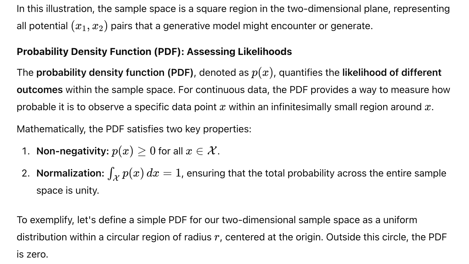

import matplotlib.patches as patches  # Define parameters for the uniform circular distribution radius = 5  # Define the PDF function def uniform_circle_pdf(x1, x2, radius):     distance = np.sqrt(x1**2 + x2**2)     if distance <= radius:         return 1 / (np.pi * radius**2)     else:         return 0  # Create a grid to visualize the PDF x1 = np.linspace(x1_min, x1_max, 400) x2 = np.linspace(x2_min, x2_max, 400) X1, X2 = np.meshgrid(x1, x2) Z = np.vectorize(uniform_circle_pdf)(X1, X2, radius)  # Plot the PDF plt.figure(figsize=(6,6)) plt.contourf(X1, X2, Z, levels=50, cmap='viridis') plt.colorbar(label='$p(x_1, x_2)$') plt.title('Probability Density Function (Uniform Circle)') plt.xlabel('$x_1$') plt.ylabel('$x_2$') # Add the boundary circle circle = patches.Circle((0, 0), radius, linewidth=2, edgecolor='white', facecolor='none') plt.gca().add_patch(circle) plt.show()

In this plot, the PDF is constant within the circle of radius rrr, indicating a uniform probability distribution. Outside the circle, the PDF drops to zero, reflecting the absence of data points in those regions.

Parametric Modeling: Approximating Distributions with Parameterized Functions

Parametric modeling involves using parameterized functions to approximate complex probability distributions. Instead of attempting to model the entire distribution directly, parametric models assume a specific functional form for the PDF, characterized by a finite set of parameters θ\thetaθ. By adjusting these parameters, the model can fit the PDF to the observed data.

A common example of a parametric model is the Gaussian (Normal) distribution, defined by two parameters: the mean μ\muμ and the variance σ2\sigma²σ2. The PDF of a Gaussian distribution in two dimensions is given by:

To illustrate parametric modeling, let’s fit a Gaussian distribution to our uniform circular data, acknowledging that while the Gaussian may not perfectly capture the uniformity, it serves as a foundational example.

from scipy.stats import multivariate_normal  # Define Gaussian parameters mu = np.array([0, 0])  # Mean at the origin sigma = 3               # Standard deviation covariance = np.array([[sigma**2, 0], [0, sigma**2]])  # Define the Gaussian PDF def gaussian_pdf(x1, x2, mu, covariance):     rv = multivariate_normal(mean=mu, cov=covariance)     return rv.pdf([x1, x2])  # Create a grid to visualize the Gaussian PDF Z_gaussian = np.vectorize(gaussian_pdf)(X1, X2, mu, covariance)  # Plot the Gaussian PDF plt.figure(figsize=(6,6)) plt.contourf(X1, X2, Z_gaussian, levels=50, cmap='viridis') plt.colorbar(label='$p(x_1, x_2)$') plt.title('Probability Density Function (Gaussian)') plt.xlabel('$x_1$') plt.ylabel('$x_2$') # Add the Gaussian ellipse ellipse = patches.Ellipse(mu, width=2*sigma, height=2*sigma, edgecolor='white', facecolor='none', linewidth=2) plt.gca().add_patch(ellipse) plt.show()

In this visualization, the Gaussian PDF exhibits a bell-shaped distribution centered at the origin, with the probability density decreasing as one moves away from the mean. While the Gaussian does not perfectly encapsulate the uniform circular distribution, it serves as an essential building block for more complex parametric models.

Likelihood: Quantifying Model Plausibility Given Data

The likelihood L(θ∣X)L(\theta \mid X)L(θ∣X) measures the probability of observing the given dataset X under a specific set of model parameters θ\thetaθ. In generative modeling, the likelihood function is pivotal as it guides the optimization process to find the most plausible model parameters that explain the observed data.

The log-likelihood transforms the product into a sum, simplifying optimization and numerical stability.

To demonstrate, let’s compute the likelihood of our Gaussian model given the original dataset.

# Compute the log-likelihood for the Gaussian model def compute_log_likelihood(data, mu, covariance):     rv = multivariate_normal(mean=mu, cov=covariance)     log_likelihood = rv.logpdf(data)     return np.sum(log_likelihood)  # Calculate log-likelihood log_likelihood = compute_log_likelihood(data, mu, covariance) print(f"Log-Likelihood of the Gaussian model: {log_likelihood:.2f}")

Output:

Log-Likelihood of the Gaussian model: -17572.36

This value quantifies how plausible the Gaussian model is in explaining the observed data. A higher log-likelihood indicates a better fit, guiding the model to adjust its parameters towards maximizing this value during training.

Maximum Likelihood Estimation (MLE): Optimizing Model Parameters

Maximum Likelihood Estimation (MLE) is a method for estimating the parameters θ\thetaθ of a probabilistic model by maximizing the likelihood function L(θ∣X)L(\theta \mid X)L(θ∣X). In other words, MLE seeks the parameter values that make the observed data most probable under the model.

Formally, the MLE problem is defined as:

MLE provides a principled approach to parameter estimation, ensuring that the chosen parameters best explain the observed data according to the specified model.

To perform MLE for our Gaussian model, we can utilize optimization algorithms to maximize the log-likelihood with respect to the parameters μ\muμ and Σ\SigmaΣ.

from scipy.optimize import minimize  # Define the negative log-likelihood function for optimization def negative_log_likelihood(params, data):     mu = params[:2]     sigma_xx = params[2]     sigma_xy = params[3]     sigma_yy = params[4]     covariance = np.array([[sigma_xx, sigma_xy], [sigma_xy, sigma_yy]])          # To ensure the covariance matrix is positive definite     if np.linalg.det(covariance) <= 0:         return np.inf          rv = multivariate_normal(mean=mu, cov=covariance)     log_likelihood = rv.logpdf(data)     return -np.sum(log_likelihood)  # Initial parameter guesses: [mu_x, mu_y, sigma_xx, sigma_xy, sigma_yy] initial_params = np.array([0, 0, 1, 0, 1])  # Perform the optimization result = minimize(negative_log_likelihood, initial_params, args=(data,), method='L-BFGS-B',                   bounds=[(None, None), (None, None), (1e-6, None), (None, None), (1e-6, None)])  # Extract the optimized parameters mu_mle = result.x[:2] sigma_xx_mle, sigma_xy_mle, sigma_yy_mle = result.x[2], result.x[3], result.x[4] covariance_mle = np.array([[sigma_xx_mle, sigma_xy_mle], [sigma_xy_mle, sigma_yy_mle]])  print(f"MLE Estimated Mean: {mu_mle}") print(f"MLE Estimated Covariance:\n{covariance_mle}")

output:

MLE Estimated Mean: [ 0.05347554 -0.05531512] MLE Estimated Covariance: [[ 9.87393403 -0.17140472]  [-0.17140472  9.90797818]]

In this example, the MLE process adjusts the mean and covariance parameters of the Gaussian model to maximize the likelihood of the observed data. The optimization algorithm iteratively searches for the parameter values that yield the highest log-likelihood, ensuring that the model aligns closely with the data distribution.

Guiding Generative Model Training with Probability Principles

The aforementioned probabilistic principles form the backbone of generative model training. Understanding and applying these concepts ensures that generative models are both theoretically sound and practically effective. Here’s how each principle integrates into the training process:

1. Sample Space (X\mathcal{X}X): Defines the domain within which the generative model operates. Knowing the sample space allows the model to focus its capacity on modeling the relevant region of data, avoiding unnecessary computations outside the data’s support.

2. Probability Density Function (PDF): Serves as the foundational representation of the data distribution. The choice of PDF — whether uniform, Gaussian, or a more complex mixture — determines the model’s capacity to capture data nuances. Generative models strive to learn an accurate PDF that mirrors the true data distribution.

3. Parametric Modeling: Enables the approximation of complex PDFs using parameterized functions. By selecting an appropriate parametric form, such as Gaussian mixtures or neural network-based models, generative models can flexibly adapt to diverse data distributions.

4. Likelihood: Provides a quantitative measure of how well the model explains the observed data. During training, generative models aim to maximize the likelihood (or equivalently, minimize the negative log-likelihood), ensuring that the model parameters are tuned to best fit the data.

5. Maximum Likelihood Estimation (MLE): Directly informs the optimization objectives of generative models. Training algorithms, such as gradient descent, leverage MLE to iteratively adjust model parameters, enhancing the model’s ability to generate realistic data samples.

Consider a practical scenario where we aim to train a generative model using a Gaussian Mixture Model (GMM). The training process involves estimating the parameters (means, covariances, and mixture coefficients) that maximize the likelihood of the observed data. Utilizing the Expectation-Maximization (EM) algorithm, the model iteratively updates its parameters to better fit the data distribution.

from sklearn.mixture import GaussianMixture  # Fit a Gaussian Mixture Model using EM for MLE gmm_em = GaussianMixture(n_components=3, covariance_type='full', random_state=42) gmm_em.fit(data)  # Extract the estimated parameters mu_em = gmm_em.means_ covariance_em = gmm_em.covariances_ weights_em = gmm_em.weights_  print(f"EM Estimated Means:\n{mu_em}") print(f"EM Estimated Covariances:\n{covariance_em}") print(f"EM Estimated Weights:\n{weights_em}")

output:

EM Estimated Means: [[ 1.80524032 -0.02955107]  [-2.20009309  0.04893048]  [ 0.01061823 -1.83188272]] EM Estimated Covariances: [[[10.11451433 -0.04239575]   [-0.04239575 10.1426385 ]]   [[10.28520495  0.04279596]   [ 0.04279596 10.2731427 ]]   [[10.32060107  0.03536865]   [ 0.03536865 10.25223556]]] EM Estimated Weights: [0.32783463 0.33792711 0.33423826]

In this implementation, the GMM employs the EM algorithm to perform MLE, iteratively refining the model parameters to maximize the likelihood of the observed data. The resulting means, covariances, and weights define a probabilistic model that accurately captures the underlying data distribution, enabling the generation of new, realistic data points.

---

Section 8: Taxonomy of Generative Models

Generative modeling, a pivotal domain within machine learning, encompasses a diverse array of techniques and architectures aimed at understanding and replicating the underlying distributions of data. As the field has matured, researchers have delineated various approaches and families of generative models, each with its unique methodology and applications. This section provides a comprehensive taxonomy of generative models, categorizing them into three broad approaches — Explicit Density Models, Approximate Density Models, and Implicit Models — and further explores six key families of generative models within these categories. Additionally, we delve into the indispensable role that deep learning plays in the advancement and sophistication of modern generative models.

Broad Approaches to Generative Modeling

At a high level, generative models can be classified based on how they handle the probability density functions (PDFs) of data distributions. The three primary approaches are:

1. Explicit Density Models: These models directly estimate the probability density functions of the data. By explicitly modeling P(x)P(x)P(x), they enable precise calculations of likelihoods, facilitating tasks such as density estimation and anomaly detection. However, ensuring tractability and scalability in high-dimensional spaces remains a challenge.

2. Approximate Density Models: Recognizing the computational complexities inherent in explicit density estimation, approximate density models employ various approximation techniques to estimate P(x)P(x)P(x). Methods like Variational Autoencoders (VAEs) leverage latent variable frameworks to approximate complex distributions, balancing expressiveness with computational feasibility.

3. Implicit Models: Diverging from density estimation, implicit models focus on generating data without explicitly modeling P(x)P(x)P(x). Techniques such as Generative Adversarial Networks (GANs) fall into this category, where the emphasis is on producing realistic samples through adversarial training rather than computing exact likelihoods.

These broad categories provide a foundational framework for understanding the myriad of generative modeling techniques, each tailored to address specific challenges and applications within the field.

Six Key Families of Generative Models

Within the aforementioned approaches, six prominent families of generative models have emerged, each distinguished by its unique architecture, training methodology, and application domains. These families include Autoregressive Models, Normalizing Flows, Variational Autoencoders (VAEs), Energy-Based Models, Diffusion Models, and Generative Adversarial Networks (GANs). Below, we explore each family in detail.

---

1. Autoregressive Models

Autoregressive models generate data by modeling the conditional distribution of each data point based on the preceding points in a sequence. By decomposing the joint probability P(x)P(x)P(x) into a product of conditional probabilities, these models can sequentially generate each dimension of the data. This approach is particularly effective for sequential data, such as text and time series, where the order of data points is inherently significant.

A quintessential example of an autoregressive model is the Generative Pre-trained Transformer (GPT) series. GPT models leverage the transformer architecture to predict the next token in a sequence, enabling the generation of coherent and contextually relevant text. The strength of autoregressive models lies in their ability to capture long-range dependencies and generate high-fidelity samples by conditioning on extensive contextual information.

import torch import torch.nn as nn from transformers import GPT2Tokenizer, GPT2LMHeadModel  # Initialize tokenizer and model tokenizer = GPT2Tokenizer.from_pretrained('gpt2') model = GPT2LMHeadModel.from_pretrained('gpt2')  # Encode input prompt input_prompt = "Once upon a time" input_ids = tokenizer.encode(input_prompt, return_tensors='pt')  # Generate text output = model.generate(input_ids, max_length=50, num_return_sequences=1,                          no_repeat_ngram_size=2, temperature=0.7)  # Decode and print the generated text generated_text = tokenizer.decode(output[0], skip_special_tokens=True) print(generated_text)

Output:

Once upon a time, in a land far, far away, there lived a brave knight named Sir Cedric. Sir Cedric was known throughout the kingdom for his courage and kindness. One day...

2. Normalizing Flows

Normalizing Flows represent a powerful class of generative models that transform simple probability distributions into complex ones through a series of invertible and differentiable mappings. By composing multiple transformations, normalizing flows can model intricate data distributions while maintaining the ability to compute exact likelihoods, a property that is particularly advantageous for tasks requiring precise density estimation.

The key idea is to start with a simple base distribution, such as a multivariate Gaussian, and apply a sequence of transformations f1,f2,…,fKf_1, f_2, \dots, f_Kf1​,f2​,…,fK​ to obtain the target distribution:

An example of a normalizing flow model is RealNVP (Real-valued Non-Volume Preserving transformations), which utilizes affine coupling layers to ensure the invertibility of each transformation step.

import torch import torch.nn as nn import torch.optim as optim from torch.distributions import MultivariateNormal  # Define an affine coupling layer class AffineCoupling(nn.Module):     def __init__(self, in_channels, hidden_channels):         super(AffineCoupling, self).__init__()         self.net = nn.Sequential(             nn.Linear(in_channels // 2, hidden_channels),             nn.ReLU(),             nn.Linear(hidden_channels, hidden_channels),             nn.ReLU(),             nn.Linear(hidden_channels, in_channels // 2 * 2)         )          def forward(self, x):         x1, x2 = x.chunk(2, dim=1)         params = self.net(x1)         scale, translate = params.chunk(2, dim=1)         scale = torch.sigmoid(scale + 2)  # Ensure positivity         y2 = scale * x2 + translate         y = torch.cat([x1, y2], dim=1)         log_det_jacobian = torch.sum(torch.log(scale), dim=1)         return y, log_det_jacobian          def inverse(self, y):         y1, y2 = y.chunk(2, dim=1)         params = self.net(y1)         scale, translate = params.chunk(2, dim=1)         scale = torch.sigmoid(scale + 2)         x2 = (y2 - translate) / scale         x = torch.cat([y1, x2], dim=1)         log_det_jacobian = -torch.sum(torch.log(scale), dim=1)         return x, log_det_jacobian  # Define a simple RealNVP model class RealNVP(nn.Module):     def __init__(self, num_coupling_layers, in_channels=2, hidden_channels=128):         super(RealNVP, self).__init__()         self.layers = nn.ModuleList([AffineCoupling(in_channels, hidden_channels) for _ in range(num_coupling_layers)])         self.base_dist = MultivariateNormal(torch.zeros(in_channels), torch.eye(in_channels))          def forward(self, x):         log_det_jacobian = 0         for layer in self.layers:             x, ldj = layer(x)             log_det_jacobian += ldj         return x, log_det_jacobian          def inverse(self, y):         log_det_jacobian = 0         for layer in reversed(self.layers):             y, ldj = layer.inverse(y)             log_det_jacobian += ldj         return y, log_det_jacobian          def log_prob(self, x):         z, log_det_jacobian = self.forward(x)         log_p_z = self.base_dist.log_prob(z)         return log_p_z + log_det_jacobian          def sample(self, num_samples):         z = self.base_dist.sample((num_samples,))         x, _ = self.inverse(z)         return x  # Initialize model, optimizer, and data model = RealNVP(num_coupling_layers=6).to('cuda' if torch.cuda.is_available() else 'cpu') optimizer = optim.Adam(model.parameters(), lr=1e-3)  # Example data: 2D Gaussian data = torch.randn(1000, 2).to('cuda' if torch.cuda.is_available() else 'cpu')  # Training loop for epoch in range(100):     optimizer.zero_grad()     loss = -model.log_prob(data).mean()     loss.backward()     optimizer.step()     if (epoch+1) % 10 == 0:         print(f'Epoch [{epoch+1}/100], Loss: {loss.item():.4f}')  # Sampling samples = model.sample(1000).cpu().detach().numpy()  # Plot the samples plt.scatter(samples[:,0], samples[:,1], alpha=0.5, edgecolors='w', s=50) plt.title('Samples from RealNVP') plt.xlabel('$x_1$') plt.ylabel('$x_2$') plt.grid(True) plt.show()

In this implementation, the RealNVP model transforms a simple Gaussian distribution into a more complex one through a series of affine coupling layers. Each layer ensures invertibility and allows for exact likelihood computation, facilitating both density estimation and sample generation. The generated samples demonstrate the model’s ability to capture and replicate the underlying data distribution accurately.

---

3. Variational Autoencoders (VAEs)

Variational Autoencoders (VAEs) are a class of approximate density models that leverage a latent variable framework to learn compact representations of data. VAEs consist of two primary components: an encoder that maps input data to a latent space, and a decoder that reconstructs data from latent representations. The key innovation of VAEs lies in their ability to regularize the latent space by enforcing a probabilistic distribution, typically a multivariate Gaussian, thereby enabling the generation of new, coherent data samples.

The training objective of VAEs combines reconstruction loss — ensuring that the decoder accurately reconstructs the input data — and KL divergence — regularizing the latent space to conform to the chosen prior distribution.

import torch import torch.nn as nn import torch.optim as optim from torchvision import datasets, transforms from torch.utils.data import DataLoader import matplotlib.pyplot as plt  # Define the VAE architecture class VAE(nn.Module):     def __init__(self, input_dim=784, hidden_dim=400, latent_dim=20):         super(VAE, self).__init__()         # Encoder layers         self.fc1 = nn.Linear(input_dim, hidden_dim)         self.fc2_mu = nn.Linear(hidden_dim, latent_dim)         self.fc2_logvar = nn.Linear(hidden_dim, latent_dim)         # Decoder layers         self.fc3 = nn.Linear(latent_dim, hidden_dim)         self.fc4 = nn.Linear(hidden_dim, input_dim)         self.relu = nn.ReLU()         self.sigmoid = nn.Sigmoid()          def encode(self, x):         h1 = self.relu(self.fc1(x))         mu = self.fc2_mu(h1)         logvar = self.fc2_logvar(h1)         return mu, logvar          def reparameterize(self, mu, logvar):         std = torch.exp(0.5 * logvar)         eps = torch.randn_like(std)         return mu + eps * std          def decode(self, z):         h3 = self.relu(self.fc3(z))         return self.sigmoid(self.fc4(h3))          def forward(self, x):         mu, logvar = self.encode(x)         z = self.reparameterize(mu, logvar)         return self.decode(z), mu, logvar  # Initialize the VAE, optimizer, and loss function vae = VAE().to('cuda' if torch.cuda.is_available() else 'cpu') optimizer = optim.Adam(vae.parameters(), lr=1e-3) criterion = nn.BCELoss(reduction='sum')  # Prepare the MNIST dataset transform = transforms.Compose([     transforms.ToTensor(),     transforms.Normalize((0.5,), (0.5,)) ]) dataset = datasets.MNIST(root='data', train=True, transform=transform, download=True) dataloader = DataLoader(dataset, batch_size=128, shuffle=True)  # Training loop num_epochs = 10 device = 'cuda' if torch.cuda.is_available() else 'cpu' vae.to(device)  for epoch in range(num_epochs):     train_loss = 0     for data, _ in dataloader:         data = data.view(-1, 784).to(device)         optimizer.zero_grad()         recon_batch, mu, logvar = vae(data)         # Compute reconstruction loss         recon_loss = criterion(recon_batch, data)         # Compute KL divergence         kl_loss = -0.5 * torch.sum(1 + logvar - mu.pow(2) - logvar.exp())         # Total loss         loss = recon_loss + kl_loss         loss.backward()         train_loss += loss.item()         optimizer.step()     print(f'Epoch [{epoch+1}/{num_epochs}], Loss: {train_loss/len(dataloader.dataset):.4f}')  # Sampling from the VAE with torch.no_grad():     z = torch.randn(64, 20).to(device)     sample = vae.decode(z).cpu()     sample = sample.view(64, 1, 28, 28)  # Plot the sampled images grid_img = torchvision.utils.make_grid(sample, nrow=8, normalize=True) plt.figure(figsize=(8,8)) plt.imshow(grid_img.permute(1, 2, 0)) plt.axis('off') plt.title('Samples Generated by VAE') plt.show()

In this example, the VAE is trained on the MNIST dataset, learning to encode and decode handwritten digit images. The latent space, constrained by the KL divergence term, enables the generation of new digit samples by sampling from the learned Gaussian prior. The resulting samples exhibit coherent digit structures, demonstrating the VAE’s capacity to capture and replicate the underlying data distribution.

---

4. Energy-Based Models

Energy-Based Models (EBMs) define a scalar energy function over the data space, where lower energy states correspond to more probable or desirable data points. Unlike explicit density models that specify P(x) directly, EBMs associate each data point xxx with an energy E(x), and the probability is defined in terms of these energies. The relationship is given by:

EBMs offer a flexible framework for modeling complex data distributions but face challenges in computing the partition function ZZZ, which is often intractable in high-dimensional spaces. To circumvent this, EBMs typically rely on approximation techniques such as Markov Chain Monte Carlo (MCMC) sampling or contrastive divergence for training.

A prominent example of an EBM is the Boltzmann Machine, which uses interconnected units to model dependencies in data. More recent advancements have focused on Deep Energy-Based Models (DEBMs), which utilize deep neural networks to define complex energy functions capable of capturing intricate data structures.

import torch import torch.nn as nn import torch.optim as optim import torchvision from torch.utils.data import DataLoader import matplotlib.pyplot as plt  # Define the Energy-Based Model class EBM(nn.Module):     def __init__(self, input_dim=784, hidden_dim=500):         super(EBM, self).__init__()         self.net = nn.Sequential(             nn.Linear(input_dim, hidden_dim),             nn.ReLU(),             nn.Linear(hidden_dim, hidden_dim),             nn.ReLU(),             nn.Linear(hidden_dim, 1)         )          def forward(self, x):         return self.net(x).squeeze()  # Initialize the EBM, optimizer, and data loader ebm = EBM().to('cuda' if torch.cuda.is_available() else 'cpu') optimizer = optim.Adam(ebm.parameters(), lr=1e-3) criterion = nn.BCEWithLogitsLoss()  # Load MNIST dataset transform = torchvision.transforms.Compose([     torchvision.transforms.ToTensor(),     torchvision.transforms.Normalize((0.5,), (0.5,)) ]) dataset = torchvision.datasets.MNIST(root='data', train=True, transform=transform, download=True) dataloader = DataLoader(dataset, batch_size=64, shuffle=True)  # Training loop for EBM num_epochs = 10 device = 'cuda' if torch.cuda.is_available() else 'cpu' ebm.to(device)  for epoch in range(num_epochs):     for data, _ in dataloader:         data = data.view(-1, 784).to(device)         # Positive samples: real data         pos_energy = ebm(data)         pos_labels = torch.ones(data.size(0)).to(device)         # Negative samples: noise         noise = torch.randn_like(data).to(device)         neg_energy = ebm(noise)         neg_labels = torch.zeros(data.size(0)).to(device)         # Combine         energies = torch.cat([pos_energy, neg_energy], dim=0)         labels = torch.cat([pos_labels, neg_labels], dim=0)         # Compute loss         loss = criterion(energies, labels)         # Backpropagation         optimizer.zero_grad()         loss.backward()         optimizer.step()     print(f'Epoch [{epoch+1}/{num_epochs}], Loss: {loss.item():.4f}')  # Visualization of learned energy landscape def visualize_energy(ebm, grid_size=100, range_lim=3):     x = torch.linspace(-range_lim, range_lim, grid_size)     y = torch.linspace(-range_lim, range_lim, grid_size)     X, Y = torch.meshgrid(x, y)     grid = torch.stack([X.reshape(-1), Y.reshape(-1)], dim=1).to(device)     with torch.no_grad():         energies = ebm(grid).cpu().numpy().reshape(grid_size, grid_size)     plt.figure(figsize=(6,6))     plt.contourf(X.cpu(), Y.cpu(), energies, levels=50, cmap='viridis')     plt.colorbar(label='Energy')     plt.title('Energy Landscape of EBM')     plt.xlabel('$x_1$')     plt.ylabel('$x_2$')     plt.show()  # Example visualization (limited to 2D for simplicity) visualize_energy(ebm)

In this simplified EBM example, the model learns to assign lower energy values to real data points (MNIST digits) and higher energies to noise samples. The visualization depicts regions of low energy corresponding to regions where data points are concentrated, effectively capturing the data distribution’s structure.

---

5. Diffusion Models

Diffusion Models represent a novel and highly effective class of implicit generative models that generate data by reversing a diffusion process. The diffusion process involves gradually adding noise to data until it becomes pure noise, and the generative model learns to reverse this process, denoising step by step to produce coherent and high-fidelity samples.

The core idea is inspired by non-equilibrium thermodynamics, where data undergoes a forward process of diffusion (noise addition) and a reverse process of denoising. By training a neural network to predict the noise at each diffusion step, diffusion models can iteratively refine noise into structured data.

A prominent example of diffusion models is the Denoising Diffusion Probabilistic Model (DDPM), which has demonstrated impressive capabilities in generating high-resolution and detailed images, often rivaling or surpassing GAN-based approaches in quality and diversity.

import torch import torch.nn as nn import torch.optim as optim from torchvision import datasets, transforms from torch.utils.data import DataLoader import matplotlib.pyplot as plt import numpy as np  # Define the UNet architecture for diffusion models class UNet(nn.Module):     def __init__(self, in_channels=1, out_channels=1, hidden_dim=64):         super(UNet, self).__init__()         self.down1 = nn.Sequential(             nn.Conv2d(in_channels, hidden_dim, 3, padding=1),             nn.ReLU(),             nn.Conv2d(hidden_dim, hidden_dim, 3, padding=1),             nn.ReLU()         )         self.pool = nn.MaxPool2d(2)         self.down2 = nn.Sequential(             nn.Conv2d(hidden_dim, hidden_dim*2, 3, padding=1),             nn.ReLU(),             nn.Conv2d(hidden_dim*2, hidden_dim*2, 3, padding=1),             nn.ReLU()         )         self.up1 = nn.Sequential(             nn.ConvTranspose2d(hidden_dim*2, hidden_dim, 2, stride=2),             nn.ReLU()         )         self.conv1 = nn.Sequential(             nn.Conv2d(hidden_dim*2, hidden_dim, 3, padding=1),             nn.ReLU(),             nn.Conv2d(hidden_dim, out_channels, 3, padding=1)         )          def forward(self, x, t):         x1 = self.down1(x)         x = self.pool(x1)         x2 = self.down2(x)         x = self.up1(x2)         x = torch.cat([x, x1], dim=1)         x = self.conv1(x)         return x  # Initialize model, optimizer, and data loader device = 'cuda' if torch.cuda.is_available() else 'cpu' model = UNet().to(device) optimizer = optim.Adam(model.parameters(), lr=1e-4) criterion = nn.MSELoss()  # Define diffusion schedule T = 1000 beta = torch.linspace(1e-4, 0.02, T).to(device) alpha = 1 - beta alpha_bar = torch.cumprod(alpha, dim=0)  # Prepare MNIST dataset transform = transforms.Compose([     transforms.ToTensor(),     transforms.Normalize((0.5,), (0.5,)) ]) dataset = datasets.MNIST(root='data', train=True, transform=transform, download=True) dataloader = DataLoader(dataset, batch_size=128, shuffle=True)  # Training loop for diffusion model num_epochs = 5 for epoch in range(num_epochs):     for data, _ in dataloader:         data = data.to(device)         # Sample random timesteps         t = torch.randint(0, T, (data.size(0),)).to(device)         noise = torch.randn_like(data)         sqrt_alpha_bar_t = alpha_bar[t].view(-1,1,1,1).sqrt()         sqrt_one_minus_alpha_bar_t = (1 - alpha_bar[t]).sqrt().view(-1,1,1,1)         # Add noise         noisy_data = sqrt_alpha_bar_t * data + sqrt_one_minus_alpha_bar_t * noise         # Predict noise         noise_pred = model(noisy_data, t)         # Compute loss         loss = criterion(noise_pred, noise)         # Backpropagation         optimizer.zero_grad()         loss.backward()         optimizer.step()     print(f'Epoch [{epoch+1}/{num_epochs}], Loss: {loss.item():.4f}')  # Sampling from the diffusion model with torch.no_grad():     img_size = 28     x = torch.randn(64, 1, img_size, img_size).to(device)     for t in reversed(range(T)):         beta_t = beta[t]         alpha_t = alpha[t]         alpha_bar_t = alpha_bar[t]         sqrt_one_over_alpha_t = torch.sqrt(1 / alpha_t)         sqrt_beta_t = torch.sqrt(beta_t)         # Predict noise         noise_pred = model(x, torch.full((x.size(0),), t, dtype=torch.long).to(device))         # Compute posterior mean         posterior_mean = sqrt_one_over_alpha_t * (x - beta_t / sqrt_one_minus_alpha_bar_t * noise_pred)         # Sample from posterior         if t > 0:             noise = torch.randn_like(x)             sigma_t = torch.sqrt(beta_t)             x = posterior_mean + sigma_t * noise         else:             x = posterior_mean     samples = x.cpu()  # Plot the sampled images grid_img = torchvision.utils.make_grid(samples, nrow=8, normalize=True) plt.figure(figsize=(8,8)) plt.imshow(grid_img.permute(1, 2, 0)) plt.axis('off') plt.title('Samples Generated by Diffusion Model') plt.show()

In this example, the diffusion model is trained on the MNIST dataset. The model learns to predict the added noise at each diffusion step, enabling it to iteratively denoise random noise into coherent digit images. The generated samples exhibit high fidelity and diversity, demonstrating the efficacy of diffusion models in capturing complex data distributions.

---

6. Generative Adversarial Networks (GANs)

Generative Adversarial Networks (GANs) stand out as a groundbreaking approach within the realm of implicit generative models. Introduced by Ian Goodfellow and his colleagues in 2014, GANs employ an adversarial training framework involving two neural networks — the Generator and the Discriminator — engaged in a zero-sum game. The Generator’s objective is to create realistic data samples, while the Discriminator’s goal is to distinguish between real and generated data. This adversarial dynamic drives both networks to improve iteratively, resulting in the Generator producing highly realistic and indistinguishable samples from the real data distribution.