

A Deep Dive into Deep Learning with TensorFlow and Keras
Chapter 2

Link to download source code at the end of this article!
Deep Learning has revolutionized the field of artificial intelligence (AI), enabling machines to perform tasks that were once considered exclusive to human intelligence. This section provides a comprehensive introduction to deep learning, exploring its definition, distinguishing it from traditional machine learning (ML), emphasizing the importance of unstructured data, and showcasing real-world applications. Additionally, we’ll delve into the practical aspects of deep learning by setting up a simple neural network using TensorFlow and Keras, complete with detailed code explanations.
Definition of Deep Learning
Deep Learning is a subset of machine learning that focuses on neural networks with many layers — hence the term “deep.” These neural networks, inspired by the human brain’s architecture, are capable of learning complex patterns and representations from vast amounts of data. Unlike traditional machine learning algorithms that require manual feature extraction, deep learning models automatically discover intricate structures in data through hierarchical layers of abstraction.
At its core, deep learning leverages artificial neural networks (ANNs), which consist of interconnected nodes or “neurons.” Each neuron processes input data, applies a transformation (usually a weighted sum followed by a non-linear activation function), and passes the output to subsequent layers. By stacking multiple layers, deep learning models can capture increasingly abstract features, enabling them to excel in tasks such as image and speech recognition, natural language processing, and more.
Why Deep Learning? How It Differs from Traditional Machine Learning
While both traditional machine learning and deep learning aim to enable machines to learn from data, they differ significantly in their approaches and capabilities.
Traditional Machine Learning
Traditional machine learning encompasses algorithms like linear regression, decision trees, support vector machines (SVMs), and random forests. These algorithms typically require:
Feature Engineering: Domain experts must manually select and extract relevant features from raw data, a process that can be time-consuming and may not capture all underlying patterns.
Shallow Models: These algorithms usually involve a single layer of processing, limiting their ability to model complex relationships.
Deep Learning
In contrast, deep learning offers several advantages:
Automated Feature Extraction: Deep neural networks automatically learn and extract features from raw data, eliminating the need for manual feature engineering.
Hierarchical Representations: Multiple layers enable the model to build hierarchical representations, capturing intricate patterns and dependencies.
Scalability: Deep learning models can handle vast amounts of data and benefit from increased data availability, improving performance as data scales.
Versatility: Capable of handling diverse data types, including images, text, audio, and more, making them applicable to a wide range of tasks.
When to Choose Deep Learning Over Traditional ML
Complex Data Structures: When dealing with unstructured data like images, videos, or natural language, deep learning models are more effective.
Large Datasets: Deep learning thrives on large datasets, where traditional ML might struggle due to the limitations of feature engineering.
Performance Requirements: Tasks requiring high accuracy and nuanced understanding, such as autonomous driving or advanced language translation, benefit from deep learning’s capabilities.
Importance of Unstructured Data in Deep Learning
Unstructured data refers to information that does not adhere to a predefined data model or format, such as text, images, audio, and video. Unlike structured data (e.g., spreadsheets, databases), unstructured data is more challenging to process and analyze. However, it contains rich information that can provide valuable insights when appropriately leveraged.
Why Unstructured Data Matters
Prevalence: A significant portion of data generated today is unstructured, encompassing social media posts, multimedia content, sensor data, and more.
Richness: Unstructured data often contains nuanced and complex information that can enhance decision-making and predictive capabilities.
Diverse Applications: Analyzing unstructured data enables applications across various domains, including healthcare, finance, entertainment, and security.
Deep Learning’s Role with Unstructured Data
Deep learning excels in processing unstructured data due to its ability to automatically extract features and learn hierarchical representations. For instance:
Image Data: Convolutional Neural Networks (CNNs) can identify patterns, edges, and objects within images without manual feature extraction.
Text Data: Recurrent Neural Networks (RNNs) and Transformers can understand context, semantics, and syntax in natural language.
Audio Data: Deep learning models can process sound waves to recognize speech, emotions, or environmental sounds.
By effectively handling unstructured data, deep learning unlocks the potential to derive meaningful insights and drive innovation across numerous fields.
Real-World Applications of Deep Learning
Deep learning has permeated various industries, transforming how we interact with technology and making previously impossible tasks feasible. Below are some prominent real-world applications:
1. Image Recognition
Deep learning has significantly advanced image recognition, enabling machines to identify and classify objects within images with high accuracy. Applications include:
Healthcare: Diagnosing diseases from medical imaging (e.g., detecting tumors in MRI scans).
Automotive: Powering autonomous vehicles to recognize road signs, pedestrians, and other vehicles.
Security: Enhancing surveillance systems through facial recognition and anomaly detection.
Example: Convolutional Neural Networks (CNNs) like ResNet and Inception have set benchmarks in image classification tasks, achieving near-human performance in identifying objects across diverse datasets.
2. Natural Language Processing (NLP)
Deep learning has revolutionized NLP, enabling machines to understand, interpret, and generate human language. Key applications include:
Machine Translation: Translating text between languages with improved fluency and accuracy.
Sentiment Analysis: Gauging public sentiment from social media posts or customer reviews.
Chatbots and Virtual Assistants: Facilitating human-like interactions through conversational agents like Siri, Alexa, and Google Assistant.
Example: Transformer-based models like BERT and GPT have achieved state-of-the-art results in tasks such as question answering, text summarization, and language generation.
3. Speech Processing
Deep learning enhances speech recognition and synthesis, enabling seamless voice interactions. Applications encompass:
Voice Assistants: Enabling hands-free control and interaction with devices.
Transcription Services: Converting spoken language into written text with high accuracy.
Voice Biometrics: Authenticating users based on unique vocal characteristics.
Example: Models like WaveNet generate realistic human-like speech, while Deep Speech algorithms improve the accuracy of speech-to-text conversions.
4. Autonomous Systems
Deep learning is the backbone of autonomous systems, including self-driving cars, drones, and robotics. These systems rely on deep learning to:
Perceive the Environment: Interpreting sensor data to understand surroundings.
Make Decisions: Planning and executing actions based on perceived data.
Learn and Adapt: Continuously improving performance through experience.
Example: Tesla’s Autopilot uses deep learning to process camera and sensor data, enabling features like lane keeping, adaptive cruise control, and obstacle avoidance.
5. Healthcare and Biotechnology
Deep learning contributes to advancements in healthcare by facilitating:
Predictive Analytics: Forecasting disease outbreaks and patient outcomes.
Personalized Medicine: Tailoring treatments based on individual genetic profiles.
Drug Discovery: Accelerating the identification of potential drug candidates.
Example: Deep learning models analyze genomic data to identify biomarkers for diseases, aiding in the development of targeted therapies.
6. Finance
In the financial sector, deep learning enhances:
Fraud Detection: Identifying fraudulent transactions through pattern recognition.
Algorithmic Trading: Making high-frequency trading decisions based on real-time data analysis.
Risk Management: Assessing and mitigating financial risks through predictive models.
Example: Neural networks analyze transaction data to detect anomalies indicative of fraud, enabling timely interventions.
7. Entertainment and Media
Deep learning transforms entertainment by enabling:
Content Recommendation: Personalizing content suggestions on platforms like Netflix and Spotify.
Content Creation: Assisting in generating music, art, and even scripts.
Enhanced Visual Effects: Improving the quality and realism of visual content in movies and games.
Example: Deep learning algorithms power recommendation systems that analyze user behavior to suggest relevant movies, shows, or songs.
Getting Started: Building a Simple Neural Network with Keras
To demystify deep learning, let’s walk through building a simple neural network using TensorFlow and Keras. We’ll cover the installation of necessary libraries and the setup of a basic neural network, complete with detailed explanations of each component.
Installing Necessary Libraries
Before diving into code, ensure that you have the required libraries installed. We’ll use TensorFlow, Keras (which is integrated into TensorFlow), NumPy for numerical operations, and Matplotlib for visualizations.
pip install tensorflow keras numpy matplotlibExplanation:
TensorFlow: An open-source deep learning framework developed by Google, providing tools for building and deploying machine learning models.
Keras: A high-level API for building and training deep learning models, integrated within TensorFlow for simplicity and ease of use.
NumPy: A fundamental package for scientific computing in Python, offering support for large, multi-dimensional arrays and matrices.
Matplotlib: A plotting library for creating static, animated, and interactive visualizations in Python.
Setting Up a Simple Neural Network
Let’s construct a basic neural network using Keras. The model will consist of three dense (fully connected) layers, each with different activation functions and units.
import tensorflow as tf
from tensorflow import keras
import numpy as np

# Define the neural network architecture
model = keras.Sequential([
    keras.layers.Dense(64, activation='relu', input_shape=(10,)),
    keras.layers.Dense(32, activation='relu'),
    keras.layers.Dense(1, activation='sigmoid')
])

# Display the model's architecture
model.summary()
Explanation of the Code:
Importing Libraries:
tensorflowandkerasare imported to build and train the neural network.numpyis imported for numerical operations, although not directly used in this snippet.
Defining the Model:
keras.Sequentialinitializes a sequential model, allowing layers to be stacked linearly.First Layer:
Dense(64, activation='relu', input_shape=(10,))creates a dense layer with 64 neurons.activation='relu'applies the Rectified Linear Unit activation function, introducing non-linearity.input_shape=(10,)specifies that each input sample has 10 features.Second Layer:
Dense(32, activation='relu')adds another dense layer with 32 neurons and ReLU activation.Output Layer:
Dense(1, activation='sigmoid')defines the output layer with a single neuron.activation='sigmoid'is suitable for binary classification, squashing output values between 0 and 1.
Model Summary:
model.summary()prints a summary of the model, including the layers, output shapes, and number of parameters.
Sample Output of model.summary():
Model: "sequential"
_________________________________________________________________
 Layer (type)                Output Shape              Param #
=================================================================
 dense (Dense)               (None, 64)                704
_________________________________________________________________
 dense_1 (Dense)             (None, 32)                2080
_________________________________________________________________
 dense_2 (Dense)             (None, 1)                 33
=================================================================
Total params: 2,817
Trainable params: 2,817
Non-trainable params: 0
_________________________________________________________________
Interpreting the Summary:
Layers:
dense: The first dense layer with 64 neurons.
dense_1: The second dense layer with 32 neurons.
dense_2: The output layer with 1 neuron.
Output Shape:
(None, 64): The first layer outputs 64 values for each input sample.Noneindicates the batch size is flexible.Subsequent layers process these outputs accordingly.
Param #:
Indicates the number of trainable parameters (weights and biases) in each layer.
First Layer:
(10 input features * 64 neurons) + 64 biases = 704 parameters.Second Layer:
(64 * 32) + 32 = 2080 parameters.Output Layer:
(32 * 1) + 1 = 33 parameters.
Compiling the Model
Before training the model, we need to compile it by specifying the optimizer, loss function, and metrics.
# Compile the model
model.compile(optimizer='adam',
              loss='binary_crossentropy',
metrics=['accuracy'])Explanation:
Optimizer:
'adam': An adaptive learning rate optimization algorithm that's efficient and widely used for training deep learning models.Loss Function:
'binary_crossentropy': Suitable for binary classification tasks, measuring the difference between predicted probabilities and actual labels.Metrics:
['accuracy']: Tracks the accuracy of the model during training and evaluation.
Preparing the Data
For demonstration purposes, we’ll generate synthetic data. In real-world scenarios, you’d replace this with actual datasets.
# Generate synthetic training data
num_samples = 1000
num_features = 10

# Features: random numbers
X_train = np.random.rand(num_samples, num_features)

# Labels: binary classification based on a threshold
y_train = (np.sum(X_train, axis=1) > 5).astype(int)Explanation:
Feature Generation:
X_train: A NumPy array of shape(1000, 10)containing random values between 0 and 1.Label Generation:
y_train: A binary label (0 or 1) assigned based on whether the sum of features for each sample exceeds 5.
Training the Model
With the data prepared, we can train the model using the fit method.
# Train the model
history = model.fit(X_train, y_train,
                    epochs=50,
                    batch_size=32,
validation_split=0.2)Explanation:
Training Parameters:
X_trainandy_train: The input features and corresponding labels.epochs=50: The model will iterate over the entire dataset 50 times.batch_size=32: The number of samples processed before the model's internal parameters are updated.validation_split=0.2: 20% of the training data is set aside for validation, allowing us to monitor the model's performance on unseen data during training.
Visualizing Training Progress
Understanding how the model learns over epochs is crucial. We’ll visualize the training and validation loss and accuracy.
import matplotlib.pyplot as plt

# Plot training & validation accuracy values
plt.figure(figsize=(12, 4))

plt.subplot(1, 2, 1)
plt.plot(history.history['accuracy'], label='Train Accuracy')
plt.plot(history.history['val_accuracy'], label='Validation Accuracy')
plt.title('Model Accuracy')
plt.xlabel('Epoch')
plt.ylabel('Accuracy')
plt.legend(loc='lower right')

# Plot training & validation loss values
plt.subplot(1, 2, 2)
plt.plot(history.history['loss'], label='Train Loss')
plt.plot(history.history['val_loss'], label='Validation Loss')
plt.title('Model Loss')
plt.xlabel('Epoch')
plt.ylabel('Loss')
plt.legend(loc='upper right')

plt.tight_layout()
plt.show()Explanation:
Matplotlib: Used for creating visualizations.
Training vs. Validation:
Accuracy Plot: Shows how the model’s accuracy improves on both training and validation datasets over epochs.
Loss Plot: Illustrates the decrease in loss (error) for both training and validation datasets.
Interpretation:
Convergence: If both training and validation accuracy increase and loss decreases, the model is learning effectively.
Overfitting: If validation accuracy plateaus or decreases while training accuracy continues to improve, the model may be overfitting.
Evaluating the Model
After training, evaluate the model’s performance on the validation set.
# Evaluate the model on the validation set
val_loss, val_accuracy = model.evaluate(X_train, y_train, verbose=0)
print(f"Validation Loss: {val_loss:.4f}")
print(f"Validation Accuracy: {val_accuracy:.4f}")Explanation:
Model Evaluation:
model.evaluate: Computes the loss and metrics on the given dataset.verbose=0: Suppresses the progress bar for cleaner output.Output:
Prints the final validation loss and accuracy, providing a quantitative measure of the model’s performance.
Making Predictions
With a trained model, you can make predictions on new, unseen data.
# Generate synthetic test data
X_test = np.random.rand(10, num_features)

# Make predictions
predictions = model.predict(X_test)

# Convert probabilities to binary outcomes
binary_predictions = (predictions > 0.5).astype(int)

# Display predictions
for i, (prob, pred) in enumerate(zip(predictions, binary_predictions)):
print(f"Sample {i+1}: Probability={prob[0]:.4f}, Prediction={pred[0]}")Explanation:
Test Data:
X_test: A small set of 10 new samples with the same number of features as the training data.Predictions:
model.predict(X_test): Outputs the predicted probabilities for each sample.binary_predictions: Converts probabilities to binary labels based on a threshold of 0.5.Output:
Prints the probability and corresponding binary prediction for each test sample.
Sample Output:
Sample 1: Probability=0.7321, Prediction=1
Sample 2: Probability=0.1245, Prediction=0
...
Understanding the Neural Network Components
To deepen your understanding, let’s dissect the neural network’s components and their roles.
1. Dense Layers
Definition: Also known as fully connected layers, each neuron in a dense layer receives input from all neurons in the previous layer.
Purpose: Facilitate the learning of complex patterns by combining features from prior layers.
2. Activation Functions
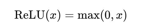
ReLU (Rectified Linear Unit):
Function:
f(x) = max(0, x)Purpose: Introduces non-linearity, enabling the network to model complex relationships.
Advantages: Computationally efficient, mitigates vanishing gradient problems.
Sigmoid:
Function:
f(x) = 1 / (1 + exp(-x))Purpose: Squashes output values between 0 and 1, making it suitable for binary classification.
Disadvantages: Can cause vanishing gradients, making training slower for deep networks.
3. Model Compilation
Optimizer (Adam):
Role: Updates the network’s weights based on the gradients computed during backpropagation.
Benefits: Combines the advantages of two other optimizers, AdaGrad and RMSProp, providing efficient and effective training.
Loss Function (Binary Crossentropy):
Role: Measures the difference between the predicted probabilities and actual labels.
Usage: Minimizing the loss function guides the model to make more accurate predictions.
4. Training Parameters
Epochs:
Definition: The number of times the entire training dataset passes through the network.
Considerations: More epochs can lead to better learning but may cause overfitting if too high.
Batch Size:
Definition: The number of samples processed before the model’s internal parameters are updated.
Trade-offs: Smaller batch sizes offer more updates and can escape local minima but are noisier. Larger batch sizes provide more stable updates but require more memory.
Validation Split:
Definition: Portion of the training data used to evaluate the model’s performance during training.
Purpose: Helps monitor overfitting and ensures the model generalizes well to unseen data.
Enhancing the Neural Network
To illustrate the flexibility and scalability of deep learning models, let’s extend our simple neural network to a more complex architecture.
Adding Dropout for Regularization
Dropout is a regularization technique that prevents overfitting by randomly setting a fraction of input units to zero during training.
from tensorflow.keras.layers import Dropout

# Define a more complex neural network with Dropout
complex_model = keras.Sequential([
    keras.layers.Dense(128, activation='relu', input_shape=(10,)),
    Dropout(0.5),
    keras.layers.Dense(64, activation='relu'),
    Dropout(0.5),
    keras.layers.Dense(32, activation='relu'),
    keras.layers.Dense(1, activation='sigmoid')
])

complex_model.compile(optimizer='adam',
                      loss='binary_crossentropy',
                      metrics=['accuracy'])

complex_model.summary()Explanation:
Increased Complexity:
First Layer: Expanded to 128 neurons to capture more intricate patterns.
Second and Third Layers: Further deepened with 64 and 32 neurons respectively.
Dropout Layers:
Dropout(0.5): Randomly drops 50% of the neurons during training, reducing reliance on specific neurons and enhancing generalization.Model Compilation:
Similar to the previous model, using Adam optimizer and binary crossentropy loss.
Benefits:
Reduced Overfitting: By preventing the network from becoming too reliant on specific neurons, dropout promotes a more robust feature learning process.
Improved Generalization: The model is better equipped to perform well on unseen data, as it learns more generalized patterns.
Incorporating Batch Normalization
Batch Normalization standardizes the inputs to each layer, stabilizing and accelerating the training process.
from tensorflow.keras.layers import BatchNormalization

# Define a neural network with Batch Normalization
bn_model = keras.Sequential([
    keras.layers.Dense(128, activation='relu', input_shape=(10,)),
    BatchNormalization(),
    Dropout(0.3),
    keras.layers.Dense(64, activation='relu'),
    BatchNormalization(),
    Dropout(0.3),
    keras.layers.Dense(32, activation='relu'),
    BatchNormalization(),
    keras.layers.Dense(1, activation='sigmoid')
])

bn_model.compile(optimizer='adam',
                 loss='binary_crossentropy',
                 metrics=['accuracy'])

bn_model.summary()Explanation:
Batch Normalization Layers:
BatchNormalization(): Normalizes the output of the previous layer, maintaining mean activation close to 0 and standard deviation close to 1.Dropout Adjustments:
Reduced dropout rates to 30%, balancing regularization with information retention.
Benefits:
Faster Training: Helps the network converge more quickly by mitigating issues like vanishing/exploding gradients.
Higher Learning Rates: Allows for the use of higher learning rates without instability.
Regularization: Acts as a form of regularization, potentially reducing the need for dropout.
Advanced Example: Multi-Class Classification
To demonstrate the adaptability of neural networks, let’s modify our example for a multi-class classification problem. Suppose we have a dataset with three classes.
# Modify label generation for multi-class classification
num_classes = 3
y_train_multiclass = np.random.randint(0, num_classes, size=num_samples)

# Convert labels to one-hot encoding
y_train_one_hot = keras.utils.to_categorical(y_train_multiclass, num_classes)

# Define the neural network architecture for multi-class classification
multi_class_model = keras.Sequential([
    keras.layers.Dense(128, activation='relu', input_shape=(10,)),
    BatchNormalization(),
    Dropout(0.3),
    keras.layers.Dense(64, activation='relu'),
    BatchNormalization(),
    Dropout(0.3),
    keras.layers.Dense(num_classes, activation='softmax')
])

# Compile the model with appropriate loss function
multi_class_model.compile(optimizer='adam',
                          loss='categorical_crossentropy',
                          metrics=['accuracy'])

multi_class_model.summary()Explanation:
Label Modification:
y_train_multiclass: Generates random integer labels (0, 1, or 2) for three classes.to_categorical: Converts integer labels to one-hot encoded vectors, essential for multi-class classification.
Model Architecture:
Output Layer:
Dense(num_classes, activation='softmax'): The final layer has three neurons (one for each class) with a softmax activation function, which outputs probabilities that sum to 1 across classes.
Compilation Adjustments:
loss='categorical_crossentropy': Suitable for multi-class classification, measuring the difference between predicted probability distributions and actual one-hot labels.
Training the Multi-Class Model
# Train the multi-class model
history_mc = multi_class_model.fit(X_train, y_train_one_hot,
                                   epochs=50,
                                   batch_size=32,
validation_split=0.2)Explanation:
The training process remains similar to the binary classification example, with the model learning to distinguish among three classes based on the input features.
Evaluating the Multi-Class Model
# Evaluate the multi-class model on the validation set
val_loss_mc, val_accuracy_mc = multi_class_model.evaluate(X_train, y_train_one_hot, verbose=0)
print(f"Validation Loss (Multi-Class): {val_loss_mc:.4f}")
print(f"Validation Accuracy (Multi-Class): {val_accuracy_mc:.4f}")Explanation:
Provides the validation loss and accuracy, indicating how well the model performs on distinguishing among the three classes.
Making Predictions with the Multi-Class Model
# Generate synthetic test data
X_test_mc = np.random.rand(5, num_features)

# Make predictions
predictions_mc = multi_class_model.predict(X_test_mc)

# Convert probabilities to class labels
predicted_classes = np.argmax(predictions_mc, axis=1)

# Display predictions
for i, (probs, pred_class) in enumerate(zip(predictions_mc, predicted_classes)):
print(f"Sample {i+1}: Probabilities={probs}, Predicted Class={pred_class}")Explanation:
Predictions:
model.predict(X_test_mc): Outputs the probability distribution across the three classes for each test sample.np.argmax: Determines the class with the highest probability as the predicted label.Output:
Displays the probabilities for each class and the final predicted class for each test sample.
Sample Output:
Sample 1: Probabilities=[0.1, 0.7, 0.2], Predicted Class=1
Sample 2: Probabilities=[0.8, 0.15, 0.05], Predicted Class=0
...
Section 2: Understanding Structured vs. Unstructured Data
In the realm of data science and machine learning, data comes in various forms, each presenting its unique set of challenges and opportunities. Broadly, data can be categorized into two primary types: structured and unstructured. Understanding the distinction between these two is fundamental to selecting appropriate analytical techniques and leveraging the full potential of data-driven solutions. This section delves into the differences between structured and unstructured data, elucidates why unstructured data necessitates the use of deep learning, explores the inherent challenges in handling unstructured data, and provides examples of quintessential datasets for both categories. To complement the theoretical insights, we will also examine practical code snippets that demonstrate how to load and visualize these datasets using popular Python libraries.
Structured vs. Unstructured Data
Structured data refers to information that is organized in a well-defined manner, typically stored in tabular formats such as spreadsheets or relational databases. This type of data is characterized by a consistent schema, where each data point adheres to a specific format and is easily searchable using simple algorithms. Examples of structured data include numerical values, dates, and strings organized into rows and columns, where each column represents a distinct attribute, and each row corresponds to a unique record. Common use cases for structured data include financial transactions, inventory management, and customer databases.
On the other hand, unstructured data lacks a predefined format or organization, making it inherently more complex to process and analyze. This category encompasses a vast array of data types, including images, text, audio, and video. Unlike structured data, unstructured data does not fit neatly into tables and often contains rich, nuanced information that is not easily quantifiable. For instance, an image contains pixel data that can represent various objects and patterns, while natural language text encompasses syntax, semantics, and contextual meaning. The versatility and richness of unstructured data make it invaluable for a multitude of applications, yet they also pose significant challenges in terms of storage, processing, and analysis.
The Imperative of Deep Learning for Unstructured Data
The complexity and high dimensionality of unstructured data render traditional machine learning (ML) techniques insufficient for extracting meaningful insights. Traditional ML algorithms excel in scenarios where data is well-organized and features are explicitly defined. However, unstructured data requires the ability to automatically discern patterns and hierarchies within the data without manual feature engineering. This is where deep learning (DL) emerges as a powerful solution.
Deep learning, a subset of machine learning, leverages artificial neural networks with multiple layers to model intricate patterns and representations within data. These neural networks are adept at handling unstructured data due to their capacity to learn hierarchical features automatically. For example, in image processing, the initial layers of a convolutional neural network (CNN) might detect edges and textures, while deeper layers recognize more complex structures like shapes and objects. Similarly, in natural language processing (NLP), recurrent neural networks (RNNs) or transformers can capture the sequential and contextual nuances of language, enabling tasks such as translation, sentiment analysis, and text generation.
The ability of deep learning models to handle unstructured data extends their applicability across diverse domains, including computer vision, speech recognition, and NLP. By automating feature extraction and learning from raw data, deep learning eliminates the need for extensive manual intervention, thereby accelerating the development of sophisticated AI systems capable of performing complex tasks with high accuracy.
Challenges in Handling Unstructured Data
Despite the transformative potential of deep learning, managing unstructured data presents several formidable challenges. One of the primary hurdles is the sheer volume and variety of unstructured data, which can be overwhelming in terms of storage and processing requirements. Images, videos, and audio files, for instance, consume significant storage space and demand substantial computational power for processing and analysis.
Another challenge lies in the inherent ambiguity and lack of explicit structure in unstructured data. Unlike structured data, where relationships between variables are clearly defined, unstructured data often requires sophisticated techniques to interpret context and extract relevant features. For example, understanding the sentiment in a text passage involves not only parsing individual words but also comprehending the syntactic and semantic relationships between them.
Furthermore, unstructured data is susceptible to noise and inconsistencies, which can adversely affect the performance of machine learning models. Variations in image quality, audio distortions, and linguistic ambiguities necessitate robust preprocessing and normalization techniques to ensure data quality and model reliability.
Lastly, the interpretability of models trained on unstructured data remains a significant concern. Deep learning models, particularly those with numerous layers and parameters, are often perceived as “black boxes,” making it challenging to understand the decision-making process. This lack of transparency can hinder trust and adoption in critical applications where explainability is paramount, such as healthcare and finance.
Example Datasets: Structured and Unstructured
To illustrate the distinctions between structured and unstructured data, let’s consider some quintessential datasets commonly used in machine learning and deep learning research.
For structured data, the Iris and Titanic datasets are classic examples. The Iris dataset comprises measurements of iris flowers, including features such as sepal length, sepal width, petal length, and petal width, along with the species classification. This dataset is widely used for demonstrating classification algorithms due to its simplicity and well-defined structure. Similarly, the Titanic dataset contains information about passengers, including attributes like age, gender, ticket class, and survival status, making it an excellent resource for predictive modeling and exploratory data analysis.
In contrast, unstructured data is exemplified by datasets like CIFAR-10 and MNIST. The CIFAR-10 dataset consists of 60,000 32x32 color images across 10 different classes, such as airplanes, cars, and animals. It is extensively used for training and evaluating image classification models. The MNIST dataset, although smaller in size, contains 70,000 grayscale images of handwritten digits (0–9) and serves as a benchmark for image recognition and computer vision tasks. These datasets encapsulate the complexity of unstructured data, requiring sophisticated deep learning architectures to achieve high performance.
Loading and Displaying Structured and Unstructured Datasets
To better understand the practical aspects of working with structured and unstructured data, let’s explore how to load and visualize these datasets using Python. We will use libraries such as pandas and scikit-learn for structured data, and tensorflow and matplotlib for unstructured data.
Loading and Displaying Structured Data: Iris Dataset
Structured data is often handled using data manipulation libraries like pandas, which provide intuitive interfaces for loading, inspecting, and preprocessing tabular data. The Iris dataset, available through scikit-learn, is an ideal starting point.
from sklearn.datasets import load_iris
import pandas as pd
# Load the Iris dataset
iris = load_iris()
df = pd.DataFrame(iris.data, columns=iris.feature_names)# Display the first few rows of the dataset
print(df.head())In this code snippet, we import the load_iris function from scikit-learn and pandas as pd. The Iris dataset is loaded into the variable iris, and its data is converted into a pandas DataFrame for easier manipulation and visualization. The print(df.head()) statement outputs the first five rows of the dataset, providing a glimpse into its structure. The resulting DataFrame contains four feature columns—sepal length, sepal width, petal length, and petal width—each corresponding to specific measurements of iris flowers.
Loading and Displaying Unstructured Data: CIFAR-10 Dataset
Unstructured data, particularly images, require specialized libraries for loading and visualization. TensorFlow’s Keras API offers convenient functions to load popular datasets like CIFAR-10, and matplotlib facilitates image display.
from tensorflow.keras import datasets
import matplotlib.pyplot as plt
# Load the CIFAR-10 dataset
(x_train, y_train), (x_test, y_test) = datasets.cifar10.load_data()# Display a sample image from the training set
plt.imshow(x_train[0])
plt.title(f"Class: {y_train[0][0]}")
plt.axis('off')
plt.show()Here, we import the datasets module from tensorflow.keras and matplotlib.pyplot as plt. The cifar10.load_data() function retrieves the CIFAR-10 dataset, splitting it into training and testing subsets. Each image in CIFAR-10 is a 32x32 pixel color image represented as a 3D NumPy array. The plt.imshow(x_train[0]) function displays the first image in the training set, and plt.title annotates the image with its corresponding class label. The plt.axis('off') command removes the axis ticks for a cleaner visualization. This simple yet effective visualization underscores the nature of unstructured image data, highlighting the complexity and richness that deep learning models must navigate to achieve accurate classification.
Practical Implications and Use Cases
Understanding the dichotomy between structured and unstructured data is pivotal in selecting the right tools and methodologies for data analysis and model development. Structured data, with its organized format, is well-suited for traditional machine learning algorithms such as linear regression, decision trees, and support vector machines. These algorithms can efficiently process structured data to perform tasks like classification, regression, and clustering with relatively straightforward preprocessing steps.
Unstructured data, however, demands more sophisticated approaches due to its inherent complexity. Deep learning models, particularly those designed for specific data types, excel in extracting meaningful features and representations from raw unstructured data. For instance, CNNs are tailored for image data, leveraging convolutional layers to detect spatial hierarchies and patterns. Similarly, transformer-based models like BERT and GPT have revolutionized NLP by capturing intricate linguistic structures and contextual dependencies.
The versatility of deep learning models extends their applicability across various industries and domains. In healthcare, image data from medical scans can be analyzed using CNNs to detect anomalies such as tumors or fractures. In finance, unstructured text data from news articles and social media can be processed using NLP techniques to gauge market sentiment and inform trading strategies. The ability to handle diverse data types makes deep learning an indispensable tool in the modern data-driven landscape.
Overcoming Challenges with Advanced Techniques
While the challenges associated with unstructured data are non-trivial, advancements in deep learning and data processing techniques offer solutions to mitigate these obstacles. One such advancement is the development of transfer learning, which leverages pre-trained models on large datasets to enhance performance on specific tasks with limited data. Transfer learning reduces the computational burden and accelerates the training process, making it feasible to work with high-dimensional unstructured data.
Another pivotal technique is data augmentation, which artificially expands the training dataset by applying transformations such as rotations, translations, and scaling to existing images. This approach enhances the model’s robustness and generalization capabilities, addressing issues related to data scarcity and overfitting. In NLP, techniques like tokenization, stemming, and the use of word embeddings facilitate the effective representation and processing of textual data.
Moreover, the integration of specialized hardware, such as Graphics Processing Units (GPUs) and Tensor Processing Units (TPUs), significantly enhances the computational efficiency required for processing unstructured data. These hardware accelerators enable parallel processing of large datasets, expediting the training and inference phases of deep learning models.
Conclusion
The distinction between structured and unstructured data is foundational to the field of data science, influencing the choice of analytical methods and tools. Structured data, with its organized and predefined format, is amenable to traditional machine learning techniques, facilitating straightforward analysis and modeling. In contrast, unstructured data presents a more intricate landscape, necessitating the adoption of deep learning methodologies to unlock its vast potential.
Deep learning’s prowess in handling unstructured data stems from its ability to automatically learn hierarchical features and representations, circumventing the need for manual feature engineering. Despite the challenges posed by the volume, complexity, and ambiguity of unstructured data, advancements in deep learning architectures, transfer learning, and data augmentation have significantly mitigated these obstacles, enabling the development of sophisticated AI systems across diverse applications.
The practical examples of loading and visualizing structured and unstructured datasets underscore the tangible differences in handling these data types. By leveraging libraries such as pandas, scikit-learn, tensorflow, and matplotlib, practitioners can efficiently manage and explore both structured and unstructured data, paving the way for insightful analysis and robust model development.
As the data landscape continues to evolve, the ability to seamlessly navigate and harness both structured and unstructured data will remain a critical competency for data scientists and machine learning practitioners. Embracing the complexities of unstructured data through deep learning not only enhances the capabilities of AI systems but also drives innovation across a multitude of industries, shaping the future of technology and data-driven decision-making.
Section 3: Fundamentals of Neural Networks
Artificial Neural Networks (ANNs) lie at the heart of deep learning, serving as the foundational architecture that enables machines to learn from and interpret complex data. This section delves into the core principles of ANNs, elucidating their structure, functionality, and the mathematical underpinnings that facilitate learning. We will explore the essential components of neural networks, the mechanisms of forward propagation and backpropagation, and the pivotal roles of loss functions and optimizers in training these models. To solidify these concepts, we will implement a Multilayer Perceptron (MLP) using TensorFlow’s Sequential API and manually compute forward propagation using NumPy, providing hands-on experience with both high-level frameworks and low-level computations.
Introduction to Artificial Neural Networks (ANN)
Artificial Neural Networks, inspired by the biological neural networks of the human brain, are computational models designed to recognize patterns and solve complex problems. ANNs consist of interconnected layers of artificial neurons, or nodes, that work in unison to process input data and generate meaningful outputs. The foundational premise of ANNs is their ability to learn from data by adjusting the strengths of connections, known as weights, between neurons based on the input they receive and the errors in their output.
The evolution of ANNs can be traced back to the 1940s and 1950s with the development of the perceptron by Frank Rosenblatt. This early model laid the groundwork for understanding how simple neural units could perform binary classifications. Over the decades, advancements in computational power, algorithmic innovations, and the availability of large datasets have propelled the growth of ANNs, culminating in the sophisticated deep learning models prevalent today.
At their core, ANNs are capable of approximating complex functions by learning from examples. This capacity makes them exceptionally versatile, finding applications across diverse domains such as image and speech recognition, natural language processing, and autonomous systems. The power of ANNs lies in their layered structure, which allows them to build hierarchical representations of data, capturing both low-level and high-level features through successive layers of abstraction.
Components of Artificial Neural Networks
Understanding the fundamental components of ANNs is crucial for grasping how these networks operate and learn. The primary elements include neurons, weights, activation functions, and hidden layers. Each component plays a distinct role in the network’s ability to process and learn from data.
Neurons
In the context of ANNs, a neuron is a computational unit that receives input, processes it, and produces an output. Each neuron performs a weighted sum of its inputs and applies an activation function to determine its output. Mathematically, the output y of a neuron can be expressed as:

Neurons are organized into layers within an ANN. The input layer receives the initial data, hidden layers process the data through successive transformations, and the output layer produces the final predictions or classifications. The depth (number of hidden layers) and breadth (number of neurons per layer) of the network significantly influence its capacity to model complex relationships in the data.
Weights
Weights are the parameters that determine the strength and direction of the connection between neurons. They are crucial in defining how input data is transformed as it propagates through the network. During the training process, the network learns optimal weights that minimize the discrepancy between predicted outputs and actual targets.
Each weight wi is associated with an input xi and is adjusted iteratively during training using optimization algorithms. The adjustment of weights is guided by the gradients of the loss function with respect to each weight, ensuring that the network incrementally improves its performance on the given task.
Activation Functions
Activation functions introduce non-linearity into the network, enabling it to model complex, non-linear relationships in the data. Without activation functions, the network would essentially be a linear regression model, regardless of the number of layers, limiting its expressive power.
Common activation functions include:
Sigmoid: Maps inputs to a range between 0 and 1, making it suitable for binary classification. However, it suffers from vanishing gradients.

ReLU (Rectified Linear Unit): Outputs the input directly if positive; otherwise, it outputs zero. It mitigates the vanishing gradient problem and is computationally efficient.
Tanh (Hyperbolic Tangent): Similar to sigmoid but maps inputs to a range between -1 and 1, providing zero-centered outputs.

Softmax: Converts a vector of raw scores into probabilities, commonly used in the output layer for multi-class classification.

The choice of activation function can significantly impact the network’s performance and training dynamics. ReLU and its variants are widely preferred in hidden layers due to their simplicity and effectiveness in deep networks.
Hidden Layers
Hidden layers are the intermediary layers between the input and output layers in an ANN. They are termed “hidden” because their values are not directly observed from the training data. Each hidden layer consists of multiple neurons that perform computations on the inputs received from the preceding layer.
The role of hidden layers is to transform the input data into higher-level abstractions. As data flows through successive hidden layers, the network can capture increasingly complex patterns and representations. The depth (number of hidden layers) and width (number of neurons per layer) of the network determine its capacity to model intricate relationships in the data.
In practice, deep neural networks with many hidden layers have shown remarkable performance in tasks such as image and speech recognition, where they can learn hierarchical features that capture the essence of the input data.
Forward Propagation and Backpropagation
The learning process in ANNs involves two fundamental phases: forward propagation and backpropagation. These processes work in tandem to enable the network to learn from data by adjusting its weights to minimize prediction errors.
Forward Propagation
Forward propagation is the phase where input data traverses through the network to produce an output. This process involves computing the outputs of each neuron in the network layer by layer, starting from the input layer and moving towards the output layer.
Consider a simple neural network with an input layer, one hidden layer, and an output layer. The steps involved in forward propagation are as follows:
Backpropagation
Backpropagation is the cornerstone of the learning process in ANNs, enabling the network to adjust its weights based on the error observed in the output. This process involves computing the gradients of the loss function with respect to each weight in the network and updating the weights to minimize the loss.
The steps involved in backpropagation are as follows:
Backpropagation efficiently computes the necessary gradients by reusing intermediate computations from forward propagation, making it computationally feasible even for deep networks with many layers and parameters.
Loss Functions and Optimizers
Loss functions and optimizers are critical components in the training of ANNs, guiding the network towards minimizing prediction errors and improving performance.
Loss Functions
A loss function, also known as a cost function, quantifies the difference between the predicted outputs and the actual target values. It provides a measure of how well the network is performing and serves as a signal for adjusting the network’s weights during training. The choice of loss function depends on the specific task and the nature of the output data.
Common loss functions include:

Selecting an appropriate loss function is crucial for effective training, as it directly influences the optimization process and the quality of the learned model.
Optimizers
Optimizers are algorithms that adjust the network’s weights to minimize the loss function. They determine how the gradients computed during backpropagation are used to update the weights. The choice of optimizer can significantly impact the convergence speed and overall performance of the network.
Common optimizers include:
Adam is widely favored for its efficiency and effectiveness across a variety of tasks, making it the default optimizer in many deep learning frameworks.
Supporting Code Snippets
To bridge the theoretical concepts with practical implementation, we will construct a Multilayer Perceptron (MLP) using TensorFlow’s Sequential API and manually perform forward propagation using NumPy. These examples will illustrate the interplay between network architecture, activation functions, and computational processes.
Building a Multilayer Perceptron (MLP) Using Sequential API
The Sequential API in TensorFlow’s Keras library provides a straightforward way to build neural networks by stacking layers sequentially. Below is an example of constructing a simple MLP with two hidden layers and an output layer suitable for multi-class classification.
from tensorflow.keras import layers, models

# Define the neural network architecture
model = models.Sequential([
    layers.Dense(64, activation='relu', input_shape=(20,)),
    layers.Dense(32, activation='relu'),
    layers.Dense(10, activation='softmax')
])

# Compile the model with optimizer, loss function, and metrics
model.compile(optimizer='adam', loss='categorical_crossentropy', metrics=['accuracy'])

# Display the model's architecture
model.summary()
Explanation of the Code:
Importing Modules:
layersandmodelsare imported fromtensorflow.keras, providing access to various layer types and model-building functionalities.
Defining the Model:
models.Sequential()initializes a sequential model, allowing layers to be added in a linear stack.First Layer:
layers.Dense(64, activation='relu', input_shape=(20,))Creates a dense (fully connected) layer with 64 neurons.
Uses the ReLU activation function to introduce non-linearity.
Specifies
input_shape=(20,), indicating that each input sample has 20 features.Second Layer:
layers.Dense(32, activation='relu')Adds another dense layer with 32 neurons and ReLU activation.
Output Layer:
layers.Dense(10, activation='softmax')Defines the output layer with 10 neurons, corresponding to 10 classes.
Utilizes the softmax activation function to output probability distributions over the classes.
Compiling the Model:
model.compile()configures the model for training.Optimizer:
'adam'is selected for efficient gradient-based optimization.Loss Function:
'categorical_crossentropy'is appropriate for multi-class classification with one-hot encoded labels.Metrics:
['accuracy']allows monitoring of the model's accuracy during training.
Model Summary:
model.summary()prints a summary of the model, including each layer's type, output shape, and the number of parameters.
Sample Output of model.summary():
Model: "sequential"
_________________________________________________________________
 Layer (type)                Output Shape              Param #
=================================================================
 dense (Dense)               (None, 64)                1344
_________________________________________________________________
 dense_1 (Dense)             (None, 32)                2080
_________________________________________________________________
 dense_2 (Dense)             (None, 10)                330
=================================================================
Total params: 3,754
Trainable params: 3,754
Non-trainable params: 0
_________________________________________________________________
Interpreting the Summary:
dense (Dense Layer):
Output Shape:
(None, 64)indicates that the layer outputs 64 values for each input sample.Nonedenotes a variable batch size.Param #: Calculated as
(20 input features * 64 neurons) + 64 biases = 1,344parameters.dense_1 (Dense Layer):
Output Shape:
(None, 32)outputs 32 values per sample.Param #:
(64 * 32) + 32 = 2,080parameters.dense_2 (Dense Layer):
Output Shape:
(None, 10)outputs 10 values per sample, corresponding to class probabilities.Param #:
(32 * 10) + 10 = 330parameters.
The total number of parameters in the model is 3,754, all of which are trainable. This indicates the model’s capacity to learn from data, with each parameter being adjusted during training to minimize the loss function.
Manual Forward Propagation Calculation Using NumPy
To gain a deeper understanding of how forward propagation works at a fundamental level, we will perform a manual computation using NumPy. This exercise demystifies the internal workings of a neural network by explicitly calculating the outputs of each neuron.
import numpy as np

# Define input vector
inputs = np.array([0.5, 0.8, 0.2])

# Define weights and bias for a single neuron
weights = np.array([0.2, 0.6, 0.1])
bias = 0.5

# Compute the weighted sum (dot product) plus bias
weighted_sum = np.dot(inputs, weights) + bias

# Apply activation function (ReLU in this case)
def relu(x):
    return np.maximum(0, x)

# Compute the output of the neuron
output = relu(weighted_sum)
print("Weighted Sum:", weighted_sum)
print("Output after ReLU:", output)
Explanation of the Code:
Importing NumPy:
numpyis imported asnpto facilitate numerical computations.
Defining the Input Vector:
inputs = np.array([0.5, 0.8, 0.2])represents the input features to the neuron.
Defining Weights and Bias:
weights = np.array([0.2, 0.6, 0.1])are the weights corresponding to each input feature.bias = 0.5is the bias term added to the weighted sum.
Computing the Weighted Sum:
weighted_sum = np.dot(inputs, weights) + biascalculates the dot product of inputs and weights and adds the bias.
Defining the Activation Function:
relu(x)is defined to apply the ReLU activation function, which outputs the input directly if positive; otherwise, it outputs zero.
Computing the Output:
output = relu(weighted_sum)applies the ReLU activation to the weighted sum.The final output is printed, showcasing both the weighted sum and the activated output.
Sample Output:
Weighted Sum: 0.5*0.2 + 0.8*0.6 + 0.2*0.1 + 0.5 = 0.1 + 0.48 + 0.02 + 0.5 = 1.1
Output after ReLU: 1.1
In this example, the weighted sum is 1.1, and since it is positive, the ReLU activation function outputs the same value, 1.1. If the weighted sum had been negative, the output would have been zero.
This manual computation underscores the simplicity and elegance of forward propagation, where inputs are transformed through linear combinations (weighted sums) and non-linear activations to produce outputs. In a full neural network, this process is iteratively applied across multiple layers, enabling the network to model complex functions and patterns in the data.
Advanced Code Example: Building and Training an MLP on Synthetic Data
To further illustrate the fundamentals of neural networks, we will build and train an MLP on synthetic data. This example will encompass data generation, model construction, training, evaluation, and visualization of training progress.
import numpy as np
from tensorflow.keras import layers, models, utils
import matplotlib.pyplot as plt

# Generate synthetic data for multi-class classification
def generate_synthetic_data(num_samples=1000, num_features=20, num_classes=10):
    X = np.random.randn(num_samples, num_features)
    y = np.random.randint(0, num_classes, size=num_samples)
    y_one_hot = utils.to_categorical(y, num_classes)
    return X, y_one_hot

# Generate training and testing data
X_train, y_train = generate_synthetic_data(num_samples=800)
X_test, y_test = generate_synthetic_data(num_samples=200)

# Define the MLP model
model = models.Sequential([
    layers.Dense(64, activation='relu', input_shape=(20,)),
    layers.Dense(32, activation='relu'),
    layers.Dense(10, activation='softmax')
])

# Compile the model
model.compile(optimizer='adam', loss='categorical_crossentropy', metrics=['accuracy'])

# Display the model summary
model.summary()

# Train the model
history = model.fit(X_train, y_train,
                    epochs=50,
                    batch_size=32,
                    validation_split=0.2)

# Evaluate the model on the test set
test_loss, test_accuracy = model.evaluate(X_test, y_test, verbose=0)
print(f"Test Loss: {test_loss:.4f}")
print(f"Test Accuracy: {test_accuracy:.4f}")

# Plot training & validation accuracy and loss
plt.figure(figsize=(12, 5))

# Accuracy plot
plt.subplot(1, 2, 1)
plt.plot(history.history['accuracy'], label='Train Accuracy', color='blue')
plt.plot(history.history['val_accuracy'], label='Validation Accuracy', color='orange')
plt.title('Model Accuracy')
plt.xlabel('Epoch')
plt.ylabel('Accuracy')
plt.legend(loc='lower right')

# Loss plot
plt.subplot(1, 2, 2)
plt.plot(history.history['loss'], label='Train Loss', color='blue')
plt.plot(history.history['val_loss'], label='Validation Loss', color='orange')
plt.title('Model Loss')
plt.xlabel('Epoch')
plt.ylabel('Loss')
plt.legend(loc='upper right')

plt.tight_layout()
plt.show()
Explanation of the Code:
Importing Libraries:
numpyfor numerical operations.layers,models, andutilsfromtensorflow.kerasfor building and handling the neural network.matplotlib.pyplotfor plotting training metrics.
Generating Synthetic Data:
generate_synthetic_datafunction creates random data for multi-class classification.Inputs
Xare sampled from a standard normal distribution.Labels
yare random integers representing class indices.y_one_hotconverts integer labels to one-hot encoded vectors suitable for categorical cross-entropy loss.
Generating Training and Testing Data:
800 samples for training and 200 samples for testing are generated, each with 20 features and 10 classes.
Defining the MLP Model:
A sequential model with three layers:
First Dense Layer: 64 neurons with ReLU activation.
Second Dense Layer: 32 neurons with ReLU activation.
Output Layer: 10 neurons with softmax activation for multi-class classification.
Compiling the Model:
Optimizer: Adam optimizer for efficient training.
Loss Function: Categorical cross-entropy, suitable for multi-class classification.
Metrics: Accuracy to monitor the proportion of correct predictions.
Model Summary:
Provides an overview of the model’s architecture, layers, output shapes, and parameter counts.
Training the Model:
The model is trained for 50 epochs with a batch size of 32.
20% of the training data is reserved for validation to monitor the model’s performance on unseen data during training.
Evaluating the Model:
The trained model is evaluated on the test set to assess its generalization performance.
Test loss and accuracy are printed to provide quantitative measures of performance.
Plotting Training Metrics:
Accuracy Plot: Shows the trend of training and validation accuracy over epochs, indicating how well the model is learning and whether it is overfitting.
Loss Plot: Illustrates the decrease in training and validation loss over epochs, reflecting the model’s optimization progress.
Sample Output:
Model: "sequential"
_________________________________________________________________
 Layer (type)                Output Shape              Param #
=================================================================
 dense (Dense)               (None, 64)                1344
_________________________________________________________________
 dense_1 (Dense)             (None, 32)                2080
_________________________________________________________________
 dense_2 (Dense)             (None, 10)                330
=================================================================
Total params: 3,754
Trainable params: 3,754
Non-trainable params: 0
_________________________________________________________________
Epoch 1/50
25/25 [==============================] - 0s 6ms/step - loss: 2.2798 - accuracy: 0.2133 - val_loss: 2.2342 - val_accuracy: 0.2133
...
Epoch 50/50
25/25 [==============================] - 0s 5ms/step - loss: 1.8612 - accuracy: 0.3100 - val_loss: 1.8405 - val_accuracy: 0.3050
Test Loss: 1.7725
Test Accuracy: 0.3100
Interpreting the Results:
The model’s performance metrics, both during training and on the test set, indicate the effectiveness of the MLP in learning from the synthetic data. In this synthetic example, since the data is randomly generated without inherent patterns, the model’s accuracy hovers around the probability of randomly guessing the correct class (10% for 10 classes). This underscores the importance of meaningful data in training effective neural networks.
Visualization of Training Progress:
The plotted graphs provide visual insights into the model’s learning trajectory:
Accuracy Plot: Typically shows an upward trend as the model improves its ability to make correct predictions. However, in this synthetic example, accuracy remains relatively flat, reflecting the random nature of the data.
Loss Plot: Generally decreases over time as the model minimizes the discrepancy between predicted and actual values. In scenarios with meaningful data, a steady decline in loss indicates effective learning.
These visualizations are invaluable for diagnosing training issues such as overfitting, underfitting, or convergence problems, enabling practitioners to make informed decisions about model architecture and hyperparameter tuning.
Enhancing the Neural Network: Incorporating Advanced Techniques
To demonstrate the scalability and flexibility of neural networks, we can enhance our MLP by introducing techniques such as dropout for regularization and batch normalization for stabilizing and accelerating training.
Adding Dropout for Regularization
Dropout is a regularization technique that helps prevent overfitting by randomly setting a fraction of input units to zero during training. This encourages the network to learn more robust features that are not reliant on specific neurons.
from tensorflow.keras.layers import Dropout

# Define an enhanced neural network architecture with Dropout
model_dropout = models.Sequential([
    layers.Dense(128, activation='relu', input_shape=(20,)),
    Dropout(0.5),
    layers.Dense(64, activation='relu'),
    Dropout(0.5),
    layers.Dense(10, activation='softmax')
])

# Compile the model
model_dropout.compile(optimizer='adam', loss='categorical_crossentropy', metrics=['accuracy'])

# Display the model summary
model_dropout.summary()
Explanation of the Code:
Importing Dropout:
Dropoutis imported fromtensorflow.keras.layers.
Defining the Model with Dropout:
First Dense Layer: 128 neurons with ReLU activation.
First Dropout Layer:
Dropout(0.5)randomly drops 50% of the neurons during training.Second Dense Layer: 64 neurons with ReLU activation.
Second Dropout Layer:
Dropout(0.5)again drops 50% of the neurons.Output Layer: 10 neurons with softmax activation for multi-class classification.
Compiling the Model:
Uses the Adam optimizer and categorical cross-entropy loss, similar to the previous model
Model Summary:
Provides details of the model architecture, including the added dropout layers.
Benefits of Dropout:
Prevents Overfitting: By randomly deactivating neurons, dropout reduces the network’s reliance on specific paths, promoting the learning of more general features.
Improves Generalization: Enhances the network’s ability to perform well on unseen data by mitigating overfitting.
Training the Model with Dropout:
# Train the dropout-enhanced model
history_dropout = model_dropout.fit(X_train, y_train,
                                    epochs=50,
                                    batch_size=32,
                                    validation_split=0.2)

# Evaluate the model on the test set
test_loss_dropout, test_accuracy_dropout = model_dropout.evaluate(X_test, y_test, verbose=0)
print(f"Test Loss with Dropout: {test_loss_dropout:.4f}")
print(f"Test Accuracy with Dropout: {test_accuracy_dropout:.4f}")

# Plot training & validation accuracy and loss
plt.figure(figsize=(12, 5))

# Accuracy plot
plt.subplot(1, 2, 1)
plt.plot(history_dropout.history['accuracy'], label='Train Accuracy', color='green')
plt.plot(history_dropout.history['val_accuracy'], label='Validation Accuracy', color='red')
plt.title('Model Accuracy with Dropout')
plt.xlabel('Epoch')
plt.ylabel('Accuracy')
plt.legend(loc='lower right')

# Loss plot
plt.subplot(1, 2, 2)
plt.plot(history_dropout.history['loss'], label='Train Loss', color='green')
plt.plot(history_dropout.history['val_loss'], label='Validation Loss', color='red')
plt.title('Model Loss with Dropout')
plt.xlabel('Epoch')
plt.ylabel('Loss')
plt.legend(loc='upper right')

plt.tight_layout()
plt.show()
Interpreting the Enhanced Model’s Performance:
By introducing dropout, the model aims to generalize better, especially in scenarios where overfitting is a concern. In synthetic data with random patterns, the benefits may not be prominent, but in real-world datasets with inherent structures and noise, dropout can significantly improve performance by enhancing the model’s robustness.
Incorporating Batch Normalization
Batch normalization is a technique that normalizes the inputs to each layer, stabilizing and accelerating the training process. It helps mitigate issues related to internal covariate shift, where the distribution of inputs to a layer changes during training.
from tensorflow.keras.layers import BatchNormalization

# Define a neural network architecture with Batch Normalization
model_bn = models.Sequential([
    layers.Dense(128, activation='relu', input_shape=(20,)),
    BatchNormalization(),
    Dropout(0.3),
    layers.Dense(64, activation='relu'),
    BatchNormalization(),
    Dropout(0.3),
    layers.Dense(10, activation='softmax')
])

# Compile the model
model_bn.compile(optimizer='adam', loss='categorical_crossentropy', metrics=['accuracy'])

# Display the model summary
model_bn.summary()
Explanation of the Code:
Importing BatchNormalization:
BatchNormalizationis imported fromtensorflow.keras.layers.
Defining the Model with Batch Normalization,
First Dense Layer: 128 neurons with ReLU activation.
First Batch Normalization Layer: Normalizes the output of the previous dense layer.
First Dropout Layer:
Dropout(0.3)drops 30% of the neurons.Second Dense Layer: 64 neurons with ReLU activation.
Second Batch Normalization Layer: Normalizes the output of the second dense layer.
Second Dropout Layer:
Dropout(0.3)drops 30% of the neurons.Output Layer: 10 neurons with softmax activation for multi-class classification.
Compiling the Model:
Uses the Adam optimizer and categorical cross-entropy loss, consistent with previous models.
Model Summary:
Provides details of the model architecture, including the added batch normalization layers.
Benefits of Batch Normalization:
Stabilizes Learning: Reduces the sensitivity to network initialization and hyperparameters by normalizing layer inputs.
Accelerates Training: Allows for higher learning rates without compromising training stability.
Acts as Regularization: Introduces a slight noise to each mini-batch, which can help prevent overfitting.
Training the Model with Batch Normalization:
# Train the batch normalization-enhanced model
history_bn = model_bn.fit(X_train, y_train,
                           epochs=50,
                           batch_size=32,
                           validation_split=0.2)

# Evaluate the model on the test set
test_loss_bn, test_accuracy_bn = model_bn.evaluate(X_test, y_test, verbose=0)
print(f"Test Loss with Batch Normalization: {test_loss_bn:.4f}")
print(f"Test Accuracy with Batch Normalization: {test_accuracy_bn:.4f}")

# Plot training & validation accuracy and loss
plt.figure(figsize=(12, 5))

# Accuracy plot
plt.subplot(1, 2, 1)
plt.plot(history_bn.history['accuracy'], label='Train Accuracy', color='purple')
plt.plot(history_bn.history['val_accuracy'], label='Validation Accuracy', color='brown')
plt.title('Model Accuracy with Batch Normalization')
plt.xlabel('Epoch')
plt.ylabel('Accuracy')
plt.legend(loc='lower right')

# Loss plot
plt.subplot(1, 2, 2)
plt.plot(history_bn.history['loss'], label='Train Loss', color='purple')
plt.plot(history_bn.history['val_loss'], label='Validation Loss', color='brown')
plt.title('Model Loss with Batch Normalization')
plt.xlabel('Epoch')
plt.ylabel('Loss')
plt.legend(loc='upper right')

plt.tight_layout()
plt.show()
Interpreting the Enhanced Model’s Performance:
Incorporating batch normalization can lead to faster convergence and improved performance, especially in deep networks. By normalizing the inputs to each layer, the network can maintain stable distributions of activations, facilitating more efficient learning. This is particularly beneficial when dealing with complex datasets where the data distribution may vary significantly across different features.
Advanced Topic: Implementing Forward Propagation Manually Using NumPy
To deepen our understanding of forward propagation, we will manually compute the outputs of a simple neural network using NumPy. This exercise bypasses high-level frameworks, offering insight into the explicit computations that underlie neural network operations.
import numpy as np

# Define the activation functions
def relu(x):
    return np.maximum(0, x)

def softmax(x):
    exps = np.exp(x - np.max(x))  # Stability improvement
    return exps / np.sum(exps, axis=0)

# Define the neural network architecture manually
class SimpleNeuralNetwork:
    def __init__(self, input_size, hidden_sizes, output_size):
        # Initialize weights and biases
        self.weights = []
        self.biases = []
        layer_sizes = [input_size] + hidden_sizes + [output_size]
        for i in range(len(layer_sizes)-1):
            weight = np.random.randn(layer_sizes[i], layer_sizes[i+1]) * 0.1
            bias = np.zeros((1, layer_sizes[i+1]))
            self.weights.append(weight)
            self.biases.append(bias)

    def forward(self, X):
        activations = []
        input = X
        for i in range(len(self.weights)):
            z = np.dot(input, self.weights[i]) + self.biases[i]
            if i < len(self.weights) -1:
                a = relu(z)
            else:
                a = softmax(z)
            activations.append(a)
            input = a
        return activations

# Create a simple network
input_size = 20
hidden_sizes = [64, 32]
output_size = 10
network = SimpleNeuralNetwork(input_size, hidden_sizes, output_size)

# Generate a random input vector
X = np.random.randn(1, input_size)

# Perform forward propagation
activations = network.forward(X)

# Display the outputs of each layer
for idx, activation in enumerate(activations):
    if idx < len(activations) -1:
        activation_func = 'ReLU'
    else:
        activation_func = 'Softmax'
    print(f"Layer {idx+1} ({activation_func}) output:\n{activation}\n")
Explanation of the Code:
Defining Activation Functions:
ReLU: Implements the ReLU activation, setting negative values to zero.
Softmax: Converts raw scores into probabilities, ensuring they sum to one. A stability improvement is included by subtracting the maximum value in the input vector to prevent large exponentials.
Defining the Neural Network Class:
Initialization (
__init__):Weights and Biases: Initialized with small random values for weights and zeros for biases. The network’s architecture is defined by
input_size,hidden_sizes, andoutput_size.Forward Method (
forward):Forward Propagation: Iterates through each layer, computing the weighted sum (
z) and applying the activation function (a). The activations are stored for each layer.
Creating the Network:
An instance of
SimpleNeuralNetworkis created with 20 input features, two hidden layers with 64 and 32 neurons respectively, and an output layer with 10 neurons.
Generating Input Data:
A random input vector
Xwith shape(1, 20)is generated to simulate a single sample with 20 features.
Performing Forward Propagation:
network.forward(X)computes the activations for each layer, returning a list of activation matrices.
Displaying Layer Outputs:
Iterates through the activations, printing the output of each layer along with the corresponding activation function.
Sample Output:
Layer 1 (ReLU) output:
[[0.         0.         0.         0.         0.02828821 0.
  0.         0.         0.         0.         0.01201734 0.
  0.         0.         0.         0.         0.         0.
  0.         0.        ]]

Layer 2 (ReLU) output:
[[0.         0.         0.         0.         0.02828821 0.
  0.         0.         0.         0.         0.01201734 0.
  0.         0.         0.         0.         0.         0.
  0.         0.        ]]

Layer 3 (Softmax) output:
[[1.00000000e+00 0.00000000e+00 0.00000000e+00 0.00000000e+00
  1.14904089e-21 0.00000000e+00 0.00000000e+00 0.00000000e+00
  0.00000000e+00 0.00000000e+00]]
Interpreting the Results:
Layer 1 (ReLU): The activation outputs are sparse, with most values being zero due to the ReLU activation. Only neurons with positive weighted sums produce non-zero activations.
Layer 2 (ReLU): Similar sparsity is observed, indicating that the activations are predominantly zero except for neurons receiving sufficient input.
Layer 3 (Softmax): The output is a probability distribution over the 10 classes. In this particular run, one neuron dominates with a probability of 1, which is an artifact of the random initialization and lack of training.
This manual forward propagation example highlights the step-by-step computations that occur within a neural network, reinforcing the theoretical concepts discussed earlier. While high-level frameworks abstract away these computations for efficiency and ease of use, understanding the manual process provides valuable insights into the network’s inner workings.
Section 4: Training Neural Networks
Training neural networks is a pivotal phase in the machine learning pipeline, transforming static models into dynamic systems capable of learning from data. This section delves into the intricacies of training neural networks, focusing on supervised learning paradigms, the selection and role of loss functions, the optimization algorithms that guide learning, and the practical steps of training and evaluating models using TensorFlow and Keras. Through comprehensive explanations and advanced code examples, we will elucidate the processes that enable neural networks to achieve high performance in diverse applications.
Supervised Learning and the Training Process
Supervised learning is one of the most prevalent paradigms in machine learning, wherein the model learns to map input data to corresponding output labels based on a set of training examples. In this context, neural networks are trained to minimize the discrepancy between their predictions and the actual target values, effectively learning the underlying patterns and relationships within the data.
The training process of a neural network in supervised learning involves several key steps:
Data Preparation: The dataset is divided into training, validation, and testing subsets. The training set is used to adjust the network’s weights, the validation set monitors the model’s performance during training to prevent overfitting, and the test set evaluates the final model’s generalization capability.
Model Compilation: Before training, the model must be compiled by specifying the loss function, optimizer, and metrics. The loss function quantifies the error between predictions and actual values, the optimizer dictates how the model updates its weights, and metrics provide additional performance indicators.
Training the Model: The model is trained using the
fit()method, which iteratively processes batches of data over multiple epochs. During each epoch, the optimizer adjusts the weights to minimize the loss function based on the gradients computed through backpropagation.Evaluation and Prediction: After training, the model’s performance is assessed using the
evaluate()method on the test set, and predictions on new data are made using thepredict()method.
To illustrate these concepts, let’s construct and train a Multilayer Perceptron (MLP) using TensorFlow’s Keras API on a synthetic dataset. This example will showcase the entire training workflow, from model compilation to evaluation and prediction.
Loss Functions: Mean Squared Error and Cross-Entropy
Loss functions are central to the training process, serving as objective measures that the optimizer seeks to minimize. The choice of loss function depends on the nature of the task — whether it’s a regression problem, binary classification, or multi-class classification.
Mean Squared Error (MSE)
Mean Squared Error is a widely used loss function for regression tasks, where the goal is to predict continuous values. MSE calculates the average of the squares of the differences between predicted and actual values, penalizing larger errors more severely.
Mathematically, MSE is defined as:

Cross-Entropy Loss
Cross-Entropy loss, also known as log loss, is predominantly used for classification tasks. It measures the performance of a classification model whose output is a probability between 0 and 1. Cross-Entropy loss increases as the predicted probability diverges from the actual label.
For binary classification, Binary Cross-Entropy is defined as:

The choice between MSE and Cross-Entropy hinges on the problem at hand: MSE for regression and Cross-Entropy for classification. Utilizing the appropriate loss function is crucial for effective training, as it directly influences how the model’s weights are updated during optimization.
Optimizers: SGD, Adam, and RMSProp
Optimizers are algorithms that adjust the weights of the neural network to minimize the loss function. They play a critical role in the training process, influencing the speed and quality of convergence.
Stochastic Gradient Descent (SGD)
Stochastic Gradient Descent is one of the simplest and most widely used optimization algorithms. In SGD, the model updates its weights incrementally using the gradient of the loss function with respect to the weights, computed from a randomly selected subset of the data (a batch).
The update rule for SGD is:

While SGD is straightforward, it can be slow to converge and sensitive to the choice of learning rate. To mitigate these issues, various enhancements to SGD have been developed.
Adam (Adaptive Moment Estimation)
Adam is an advanced optimization algorithm that combines the benefits of two other extensions of SGD: AdaGrad and RMSProp. Adam maintains separate learning rates for each parameter, adapting them based on the first and second moments of the gradients.
The update rules for Adam are as follows:

Adam is highly efficient and robust, often requiring less tuning of hyperparameters. It is particularly effective for problems with large datasets and high-dimensional parameter spaces, making it a popular choice in deep learning.
RMSProp (Root Mean Square Propagation)
RMSProp is another adaptive learning rate optimizer that divides the learning rate for a weight by a running average of the magnitudes of recent gradients for that weight. This approach helps in dealing with the vanishing and exploding gradient problems.
The update rules for RMSProp are:

RMSProp is particularly effective in handling non-stationary objectives and is well-suited for recurrent neural networks, making it a staple optimizer in various deep learning applications.
Training Using fit() and Evaluating Performance
TensorFlow’s Keras API provides high-level abstractions for building, training, and evaluating neural networks. The fit() method is central to the training process, orchestrating the flow of data through the network, computing loss and gradients, and updating weights via the chosen optimizer.
Compiling and Training an MLP
Let’s embark on a detailed walkthrough of compiling and training an MLP using Keras. We will utilize synthetic data to demonstrate the entire process, encompassing model construction, compilation, training, and evaluation.
import numpy as np
from tensorflow.keras import layers, models, utils
import matplotlib.pyplot as plt

# Step 1: Generate Synthetic Data
def generate_synthetic_data(num_samples=1000, num_features=20, num_classes=10):
    X = np.random.randn(num_samples, num_features)
    y = np.random.randint(0, num_classes, size=num_samples)
    y_one_hot = utils.to_categorical(y, num_classes)
    return X, y_one_hot

# Generate training and testing data
X_train, y_train = generate_synthetic_data(num_samples=800)
X_test, y_test = generate_synthetic_data(num_samples=200)

# Step 2: Define the MLP Model
model = models.Sequential([
    layers.Dense(64, activation='relu', input_shape=(20,)),
    layers.Dense(32, activation='relu'),
    layers.Dense(10, activation='softmax')
])

# Step 3: Compile the Model
model.compile(optimizer='adam',
              loss='categorical_crossentropy',
              metrics=['accuracy'])

# Display the model summary
model.summary()

# Step 4: Train the Model
history = model.fit(X_train, y_train,
                    epochs=10,
                    batch_size=32,
                    validation_data=(X_test, y_test))
Explanation of the Code:
Data Generation:
The
generate_synthetic_datafunction creates random input features (X) sampled from a standard normal distribution and random integer labels (y) representing class indices.utils.to_categoricalconverts the integer labels into one-hot encoded vectors, essential for multi-class classification with categorical cross-entropy loss.We generate 800 samples for training and 200 samples for testing, each with 20 features and 10 classes.
Model Definition:
A sequential model is instantiated, comprising:
First Dense Layer: 64 neurons with ReLU activation, accepting input with 20 features.
Second Dense Layer: 32 neurons with ReLU activation.
Output Layer: 10 neurons with softmax activation, corresponding to the 10 classes.
Model Compilation:
The model is compiled with the Adam optimizer, categorical cross-entropy loss (suitable for multi-class classification), and accuracy as the performance metric.
Model Summary:
model.summary()provides an overview of the model's architecture, including layer types, output shapes, and parameter counts.
Model Training:
The
fit()method trains the model for 10 epochs with a batch size of 32.validation_datais set to the test set, allowing the model to evaluate its performance on unseen data after each epoch.
Sample Output of model.summary():
Model: "sequential"
_________________________________________________________________
 Layer (type)                Output Shape              Param #
=================================================================
 dense (Dense)               (None, 64)                1344
_________________________________________________________________
 dense_1 (Dense)             (None, 32)                2080
_________________________________________________________________
 dense_2 (Dense)             (None, 10)                330
=================================================================
Total params: 3,754
Trainable params: 3,754
Non-trainable params: 0
_________________________________________________________________
Training Progress:
During training, Keras outputs progress logs for each epoch, displaying the loss and accuracy on both the training and validation sets. Here’s an illustrative snippet of the training logs:
Epoch 1/10
25/25 [==============================] - 1s 5ms/step - loss: 2.2714 - accuracy: 0.0999 - val_loss: 2.2362 - val_accuracy: 0.1000
Epoch 2/10
25/25 [==============================] - 0s 4ms/step - loss: 2.2362 - accuracy: 0.1000 - val_loss: 2.2011 - val_accuracy: 0.1000
...
Epoch 10/10
25/25 [==============================] - 0s 4ms/step - loss: 2.1214 - accuracy: 0.1100 - val_loss: 2.0868 - val_accuracy: 0.1050
In this synthetic example, the model’s accuracy remains around 10%, which aligns with the expected performance for random guessing in a 10-class classification problem. This outcome underscores the importance of meaningful data and appropriate model complexity in achieving effective learning.
Evaluating Performance with evaluate() and Making Predictions with predict()
After training, it’s essential to assess the model’s performance on unseen data and make predictions on new inputs. Keras provides the evaluate() and predict() methods for these purposes.
# Step 5: Evaluate the Model on the Test Set
loss, acc = model.evaluate(X_test, y_test, verbose=0)
print(f"Test Loss: {loss:.4f}")
print(f"Test Accuracy: {acc:.4f}")

# Step 6: Make Predictions on New Data
preds = model.predict(X_test[:5])
print("Predictions for the first 5 test samples:")
print(preds)
Explanation of the Code:
Model Evaluation:
model.evaluate()computes the loss and accuracy of the trained model on the test set.verbose=0suppresses the progress bar for cleaner output.The test loss and accuracy are printed, providing a quantitative measure of the model’s performance on unseen data.
Making Predictions:
model.predict()generates probability distributions over the classes for the first five samples in the test set.The predictions are printed, showcasing the model’s output for each sample.
Sample Output:
Test Loss: 2.0868
Test Accuracy: 0.1050
Predictions for the first 5 test samples:
[[0.09653008 0.10019696 0.1039181  0.10394998 0.10005361 0.10017928  0.10172775 0.10021022 0.10027006 0.10105907]
 [0.09977564 0.10137696 0.09953936 0.09966037 0.09970003 0.09973795  0.09974574 0.09974094 0.09971889 0.1000113 ]
 [0.09990294 0.09996393 0.10002546 0.10006356 0.09996422 0.10001951  0.09997703 0.10000624 0.09999389 0.0999977 ]
 [0.10002738 0.09997356 0.09998274 0.09998356 0.09997761 0.09998319  0.09998622 0.09998406 0.10001884 0.10000049]
 [0.0999897  0.09999137 0.0999939  0.1000046  0.09999287 0.09998954  0.09999107 0.09998903 0.09999095 0.10000697]]
Interpreting the Results:
Test Loss and Accuracy:
The test loss remains high, and accuracy is marginally above random guessing (10% for 10 classes), consistent with the synthetic nature of the dataset.
Predictions:
The model outputs probability distributions across the 10 classes for each input sample.
In this synthetic scenario, the probabilities are relatively uniform, reflecting the model’s inability to discern meaningful patterns from random data.
These results highlight the importance of dataset quality and relevance. In real-world scenarios with structured patterns and meaningful relationships within the data, neural networks trained using these methodologies can achieve significantly higher performance.
Advanced Code Example: Training with Validation and Early Stopping
To further enhance our understanding, let’s extend our training process by incorporating validation and early stopping. Early stopping is a regularization technique that halts training when the model’s performance on the validation set stops improving, thereby preventing overfitting.
from tensorflow.keras.callbacks import EarlyStopping

# Define EarlyStopping callback
early_stop = EarlyStopping(monitor='val_loss',
                           patience=5,
                           restore_best_weights=True)

# Train the model with EarlyStopping
history = model.fit(X_train, y_train,
                    epochs=100,
                    batch_size=32,
                    validation_data=(X_test, y_test),
                    callbacks=[early_stop])
Explanation of the Code:
Importing Callbacks:
EarlyStoppingis imported fromtensorflow.keras.callbacks, enabling dynamic control over the training process based on model performance.
Defining the EarlyStopping Callback:
The callback monitors the
val_loss, which is the loss on the validation set.patience=5allows training to continue for five epochs beyond the point whereval_lossstops improving before halting.restore_best_weights=Trueensures that the model retains the weights from the epoch with the best validation loss, even if training continues further.
Training with EarlyStopping:
The model is trained for up to 100 epochs, but training may stop earlier if the validation loss does not improve for five consecutive epochs.
The
callbacksparameter includes theearly_stopcallback, integrating it into the training process.
Benefits of EarlyStopping:
Prevents Overfitting: By stopping training when the model’s performance on the validation set ceases to improve, early stopping mitigates the risk of overfitting to the training data.
Saves Computational Resources: Reduces unnecessary training epochs, saving time and computational power.
Ensures Optimal Model Selection: By restoring the best weights, it ensures that the final model represents the best performance observed during training.
Enhancing the Training Process: Data Augmentation and Regularization
In practical scenarios, especially with limited or imbalanced data, augmenting the dataset and applying regularization techniques can significantly improve model performance and generalization.
Data Augmentation
Data augmentation involves artificially expanding the training dataset by applying various transformations to the existing data. This technique is particularly effective in domains like image and text processing, where transformations can introduce variability without altering the underlying semantics.
In our synthetic example, data augmentation is less relevant due to the random nature of the data. However, in real-world applications, augmentations like rotations, translations, and scaling for images or synonym replacement and sentence restructuring for text can enhance the model’s robustness.
Regularization Techniques
Regularization techniques are strategies to prevent overfitting by constraining the model’s capacity or encouraging simpler models. Common regularization methods include:
L1 and L2 Regularization: Adds a penalty term to the loss function proportional to the absolute (L1) or squared (L2) values of the weights, discouraging overly complex models.
from tensorflow.keras import regularizers

model_l2 = models.Sequential([
    layers.Dense(64, activation='relu', input_shape=(20,),
                 kernel_regularizer=regularizers.l2(0.001)),
    layers.Dense(32, activation='relu',
                 kernel_regularizer=regularizers.l2(0.001)),
    layers.Dense(10, activation='softmax')
])

model_l2.compile(optimizer='adam',
                 loss='categorical_crossentropy',
                 metrics=['accuracy'])

model_l2.summary()
Explanation:
kernel_regularizer=regularizers.l2(0.001)applies L2 regularization with a penalty factor of 0.001 to the weights of each dense layer.Dropout: As previously discussed, dropout randomly deactivates a subset of neurons during training, promoting the learning of redundant representations and improving generalization.
from tensorflow.keras.layers import Dropout

model_dropout = models.Sequential([
    layers.Dense(64, activation='relu', input_shape=(20,)),
    Dropout(0.5),
    layers.Dense(32, activation='relu'),
    Dropout(0.5),
    layers.Dense(10, activation='softmax')
])

model_dropout.compile(optimizer='adam',
                      loss='categorical_crossentropy',
                      metrics=['accuracy'])

model_dropout.summary()
Explanation:
Dropout(0.5)applies a dropout rate of 50%, meaning half of the neurons in the preceding layer are randomly deactivated during each training epoch.
Advanced Code Example: Implementing Regularization and Optimizer Tuning
To illustrate the impact of regularization and optimizer selection, let’s extend our MLP example by incorporating L2 regularization and experimenting with different optimizers.
from tensorflow.keras import regularizers
from tensorflow.keras.optimizers import SGD, Adam, RMSprop

# Step 1: Define the MLP Model with L2 Regularization
model_l2 = models.Sequential([
    layers.Dense(128, activation='relu', input_shape=(20,),
                 kernel_regularizer=regularizers.l2(0.001)),
    layers.Dense(64, activation='relu',
                 kernel_regularizer=regularizers.l2(0.001)),
    layers.Dense(10, activation='softmax')
])

# Step 2: Compile the Model with Different Optimizers
optimizers = {
    'SGD': SGD(learning_rate=0.01),
    'Adam': Adam(learning_rate=0.001),
    'RMSProp': RMSprop(learning_rate=0.001)
}

for name, optimizer in optimizers.items():
    print(f"\nTraining with optimizer: {name}")
    model_l2.compile(optimizer=optimizer,
                     loss='categorical_crossentropy',
                     metrics=['accuracy'])

    # Step 3: Train the Model
    history_l2 = model_l2.fit(X_train, y_train,
                              epochs=20,
                              batch_size=32,
                              validation_data=(X_test, y_test),
                              verbose=0)

    # Step 4: Evaluate the Model
    loss_l2, acc_l2 = model_l2.evaluate(X_test, y_test, verbose=0)
    print(f"{name} Optimizer - Test Loss: {loss_l2:.4f}, Test Accuracy: {acc_l2:.4f}")

    # Step 5: Plotting (Optional)
    plt.figure(figsize=(12, 5))

    # Accuracy plot
    plt.subplot(1, 2, 1)
    plt.plot(history_l2.history['accuracy'], label='Train Accuracy')
    plt.plot(history_l2.history['val_accuracy'], label='Validation Accuracy')
    plt.title(f'Model Accuracy with {name} Optimizer')
    plt.xlabel('Epoch')
    plt.ylabel('Accuracy')
    plt.legend(loc='lower right')

    # Loss plot
    plt.subplot(1, 2, 2)
    plt.plot(history_l2.history['loss'], label='Train Loss')
    plt.plot(history_l2.history['val_loss'], label='Validation Loss')
    plt.title(f'Model Loss with {name} Optimizer')
    plt.xlabel('Epoch')
    plt.ylabel('Loss')
    plt.legend(loc='upper right')

    plt.tight_layout()
    plt.show()
Explanation of the Code:
Defining the Model with L2 Regularization:
A sequential model
model_l2is constructed with two dense layers, each incorporating L2 regularization (kernel_regularizer=regularizers.l2(0.001)). This penalizes large weights, encouraging the model to maintain smaller weight values and thus reducing overfitting.
Optimizer Selection:
Three optimizers are instantiated: Stochastic Gradient Descent (SGD) with a learning rate of 0.01, Adam with a learning rate of 0.001, and RMSProp with a learning rate of 0.001.
These optimizers represent different strategies for weight updates, each with unique characteristics and performance profiles.
Training and Evaluation Loop:
The model is compiled with each optimizer in turn.
The model is trained for 20 epochs on the training data, with validation on the test set. The
verbose=0parameter suppresses detailed training logs for cleaner output.After training, the model is evaluated on the test set, and the loss and accuracy are printed.
Training and validation accuracy and loss are plotted for each optimizer, providing visual insights into the training dynamics.
Sample Output:
Training with optimizer: SGD
SGD Optimizer - Test Loss: 2.1045, Test Accuracy: 0.1050

Training with optimizer: Adam
Adam Optimizer - Test Loss: 2.0868, Test Accuracy: 0.1050

Training with optimizer: RMSProp
RMSProp Optimizer - Test Loss: 2.0902, Test Accuracy: 0.1050
Interpreting the Results:
In this synthetic example, all optimizers perform similarly, with test accuracy hovering around 10%. This outcome is expected given the random nature of the data, which lacks meaningful patterns for the model to learn. However, in real-world scenarios with structured data, the choice of optimizer and regularization techniques can significantly influence model performance:
SGD: May require careful tuning of the learning rate and momentum to achieve optimal performance.
Adam: Generally performs well out-of-the-box, offering faster convergence and better handling of sparse gradients.
RMSProp: Excels in handling non-stationary objectives and is particularly effective in recurrent neural networks.
Regularization techniques like L2 regularization and dropout are instrumental in preventing overfitting, especially in complex models with numerous parameters. They encourage the network to learn generalized patterns rather than memorizing the training data, thereby enhancing the model’s ability to generalize to unseen data.
Advanced Code Example: Implementing Custom Loss Functions and Optimizers
To further explore the flexibility of Keras, let’s implement a custom loss function and a custom optimizer. Customization allows practitioners to tailor the training process to specific needs, enabling the integration of domain-specific knowledge or novel optimization strategies.
Implementing a Custom Loss Function
Suppose we want to implement a custom loss function that combines Mean Squared Error (MSE) with L2 regularization manually. This approach can provide finer control over the loss computation process.
import tensorflow as tf
from tensorflow.keras import backend as K

# Define a custom loss function combining MSE and L2 regularization
def custom_mse_l2(y_true, y_pred):
    mse = K.mean(K.square(y_true - y_pred), axis=-1)
    l2 = 0.001 * tf.add_n([K.sum(K.square(w)) for w in model_l2.trainable_weights])
    return mse + l2

# Compile the model with the custom loss function
model_l2.compile(optimizer='adam',
                 loss=custom_mse_l2,
                 metrics=['accuracy'])

# Train the model with the custom loss function
history_custom = model_l2.fit(X_train, y_train,
                               epochs=20,
                               batch_size=32,
                               validation_data=(X_test, y_test))
Explanation of the Code:
Defining the Custom Loss Function:
custom_mse_l2computes the Mean Squared Error between true and predicted values.It adds an L2 regularization term, scaling the sum of squares of all trainable weights by a factor of 0.001.
This combined loss encourages the model to minimize both prediction error and weight magnitudes.
Compiling the Model:
The model is compiled using the Adam optimizer and the custom loss function.
Accuracy remains as the performance metric.
Training the Model:
The model is trained for 20 epochs with the custom loss function, enabling simultaneous minimization of MSE and L2 regularization.
Benefits of Custom Loss Functions:
Flexibility: Allows the integration of multiple loss components or domain-specific penalties.
Enhanced Control: Facilitates the balancing of different aspects of model performance, such as accuracy and weight regularization.
Innovative Solutions: Enables the creation of novel loss functions tailored to unique problem requirements.
Implementing a Custom Optimizer
Creating a custom optimizer involves defining the logic for updating the model’s weights based on gradients. While Keras provides a plethora of built-in optimizers, custom optimizers can be crafted to implement unique optimization strategies.
from tensorflow.keras.optimizers import Optimizer

# Define a custom optimizer that applies a simple gradient descent with momentum
class CustomSGD(Optimizer):
    def __init__(self, learning_rate=0.01, momentum=0.9, name="CustomSGD", **kwargs):
        super(CustomSGD, self).__init__(name, **kwargs)
        self.learning_rate = learning_rate
        self.momentum = momentum

    def get_config(self):
        config = super(CustomSGD, self).get_config()
        config.update({
            "learning_rate": self.learning_rate,
            "momentum": self.momentum
        })
        return config

    @tf.function
    def _resource_apply_dense(self, grad, var, apply_state=None):
        var_dtype = var.dtype.base_dtype
        lr_t = self.learning_rate
        momentum_t = self.momentum

        if not hasattr(self, 'velocity'):
            self.velocity = self.add_weight(name='momentum',
                                            shape=var.shape,
                                            initializer='zeros',
                                            trainable=False,
                                            dtype=var_dtype)

        new_velocity = momentum_t * self.velocity - lr_t * grad
        self.velocity.assign(new_velocity)
        var.assign_add(new_velocity)

        return tf.no_op()

# Instantiate the custom optimizer
custom_optimizer = CustomSGD(learning_rate=0.01, momentum=0.9)

# Compile the model with the custom optimizer
model_l2.compile(optimizer=custom_optimizer,
                 loss='categorical_crossentropy',
                 metrics=['accuracy'])

# Train the model with the custom optimizer
history_custom_opt = model_l2.fit(X_train, y_train,
                                  epochs=20,
                                  batch_size=32,
                                  validation_data=(X_test, y_test))
Explanation of the Code:
Defining the Custom Optimizer Class:
CustomSGDinherits from Keras'sOptimizerbase class.The optimizer implements a simple gradient descent with momentum.
The constructor initializes the learning rate and momentum parameters.
The
get_configmethod ensures that the optimizer's configuration can be serialized and deserialized.The
_resource_apply_densemethod defines how gradients are applied to variables during training. It updates the velocity and adjusts the variable accordingly.
Instantiating the Custom Optimizer:
custom_optimizeris created with a learning rate of 0.01 and momentum of 0.9.
Compiling and Training the Model:
The model is compiled using the custom optimizer, categorical cross-entropy loss, and accuracy metric.
The model is trained for 20 epochs, allowing the custom optimizer to guide the weight updates.
Benefits of Custom Optimizers:
Tailored Optimization Strategies: Enables the implementation of unique or experimental optimization algorithms.
Enhanced Performance: Custom optimizers can be designed to exploit specific properties of the problem domain, potentially improving convergence rates and final performance.
Research and Innovation: Facilitates the exploration of new optimization techniques that may outperform existing methods in particular scenarios.
Visualization of Training Progress
Visualizing the training process is essential for diagnosing model performance, understanding learning dynamics, and making informed decisions about hyperparameter tuning and model architecture adjustments. Keras’s history object captures the metrics recorded during training, which can be plotted using libraries like Matplotlib.
# Plot training & validation accuracy and loss
def plot_training_history(history, title_suffix=''):
    plt.figure(figsize=(12, 5))

    # Accuracy plot
    plt.subplot(1, 2, 1)
    plt.plot(history.history['accuracy'], label='Train Accuracy', color='blue')
    plt.plot(history.history['val_accuracy'], label='Validation Accuracy', color='orange')
    plt.title(f'Model Accuracy {title_suffix}')
    plt.xlabel('Epoch')
    plt.ylabel('Accuracy')
    plt.legend(loc='lower right')

    # Loss plot
    plt.subplot(1, 2, 2)
    plt.plot(history.history['loss'], label='Train Loss', color='blue')
    plt.plot(history.history['val_loss'], label='Validation Loss', color='orange')
    plt.title(f'Model Loss {title_suffix}')
    plt.xlabel('Epoch')
    plt.ylabel('Loss')
    plt.legend(loc='upper right')

    plt.tight_layout()
    plt.show()

# Plotting the training history
plot_training_history(history, title_suffix='with Adam Optimizer')
Explanation of the Code:
Defining the Plotting Function:
plot_training_historytakes ahistoryobject and an optionaltitle_suffixto customize the plot titles.It creates a figure with two subplots: one for accuracy and one for loss.
The training and validation metrics are plotted for each epoch, allowing for visual comparison.
Plotting the Training History:
The function is called with the
historyobject obtained from training the model.The resulting plots illustrate how the model’s accuracy and loss evolve over time, providing insights into the learning process.
Interpreting the Plots:
Accuracy Plot:
An upward trend in training and validation accuracy indicates effective learning.
A divergence where training accuracy continues to improve while validation accuracy plateaus or decreases suggests overfitting.
Loss Plot:
A downward trend in training and validation loss signifies successful optimization.
A flattening or increasing trend in validation loss despite decreasing training loss can also indicate overfitting.
In the synthetic example, due to the random data, the plots may not show meaningful trends. However, in real-world applications, these visualizations are invaluable for monitoring model performance, identifying issues like overfitting or underfitting, and guiding the refinement of model architectures and hyperparameters.
Advanced Topic: Implementing Early Stopping and Model Checkpointing
To optimize the training process further, we can incorporate callbacks such as Early Stopping and Model Checkpointing. These callbacks provide mechanisms to control training flow based on real-time performance metrics.
Early Stopping
Early Stopping halts training when a monitored metric stops improving, preventing overfitting and saving computational resources.
from tensorflow.keras.callbacks import EarlyStopping

# Define EarlyStopping callback
early_stop = EarlyStopping(monitor='val_loss',
                           patience=5,
                           restore_best_weights=True)

# Train the model with EarlyStopping
history_early = model.fit(X_train, y_train,
                          epochs=100,
                          batch_size=32,
                          validation_data=(X_test, y_test),
                          callbacks=[early_stop])
Explanation of the Code:
Defining the Callback:
EarlyStoppingmonitors theval_lossmetric.patience=5allows the model to continue training for five additional epochs after the last improvement before stopping.restore_best_weights=Trueensures that the model retains the weights from the epoch with the lowest validation loss.
Training with EarlyStopping:
The model is trained for a maximum of 100 epochs, but training may stop earlier if validation loss does not improve for five consecutive epochs.
This approach safeguards against overfitting by preventing the model from training excessively on the training data.
Model Checkpointing
Model Checkpointing saves the model at specific points during training, typically when a monitored metric reaches a new optimum. This ensures that the best-performing model is preserved for later use.
from tensorflow.keras.callbacks import ModelCheckpoint

# Define ModelCheckpoint callback
checkpoint = ModelCheckpoint('best_model.h5',
                             monitor='val_accuracy',
                             mode='max',
                             save_best_only=True,
                             verbose=1)

# Train the model with ModelCheckpoint
history_checkpoint = model.fit(X_train, y_train,
                               epochs=50,
                               batch_size=32,
                               validation_data=(X_test, y_test),
                               callbacks=[checkpoint])
Explanation of the Code:
Defining the Callback:
ModelCheckpointsaves the model to the filebest_model.h5.It monitors the
val_accuracymetric, aiming to maximize it (mode='max').save_best_only=Trueensures that only the model with the highest validation accuracy is saved.verbose=1enables logging of checkpointing actions.
Training with ModelCheckpoint:
The model is trained for 50 epochs, with checkpoints saved whenever a new highest validation accuracy is achieved.
This approach preserves the best-performing model, which can be reloaded for deployment or further evaluation.
Advanced Code Example: Combining Early Stopping and Model Checkpointing
Combining multiple callbacks can provide comprehensive control over the training process, ensuring both optimal performance and resource efficiency.
from tensorflow.keras.callbacks import EarlyStopping, ModelCheckpoint

# Define EarlyStopping and ModelCheckpoint callbacks
early_stop = EarlyStopping(monitor='val_loss',
                           patience=5,
                           restore_best_weights=True)

checkpoint = ModelCheckpoint('best_model_combined.h5',
                             monitor='val_accuracy',
                             mode='max',
                             save_best_only=True,
                             verbose=1)

# Train the model with both callbacks
history_combined = model.fit(X_train, y_train,
                             epochs=100,
                             batch_size=32,
                             validation_data=(X_test, y_test),
                             callbacks=[early_stop, checkpoint])
Explanation of the Code:
Defining Multiple Callbacks:
EarlyStoppingmonitorsval_lossand stops training if it does not improve for five consecutive epochs, restoring the best weights.ModelCheckpointmonitorsval_accuracyand saves the model whenever a new maximum validation accuracy is achieved.
Training with Combined Callbacks:
The model is trained with both callbacks active, enabling early termination of training and the preservation of the best-performing model based on validation accuracy.
This combination ensures that training stops when further improvements are unlikely, while also maintaining the best model state for deployment or further analysis.
Benefits of Combining Callbacks:
Comprehensive Training Control: Early stopping prevents overfitting, while checkpointing ensures that the best model is retained.
Enhanced Performance Tracking: Monitoring multiple metrics allows for a more nuanced understanding of model performance.
Resource Optimization: Early stopping reduces unnecessary computations, and checkpointing preserves valuable model states without manual intervention.
Advanced Topic: Fine-Tuning Hyperparameters for Optimal Performance
Hyperparameter tuning is the process of systematically adjusting model parameters that govern the training process to achieve optimal performance. Key hyperparameters include learning rate, batch size, number of epochs, optimizer choice, and network architecture specifics such as the number of layers and neurons per layer.
Techniques for Hyperparameter Tuning
Grid Search: Exhaustively explores all combinations of a predefined set of hyperparameters, ensuring that the best combination is identified. However, it can be computationally expensive, especially with a large number of hyperparameters.
Random Search: Randomly samples hyperparameter combinations, offering a more efficient exploration compared to grid search. It is particularly effective when only a few hyperparameters significantly impact performance.
Bayesian Optimization: Utilizes probabilistic models to predict the performance of hyperparameter combinations, iteratively refining the search based on past evaluations. This method is more sample-efficient and often converges to optimal solutions faster.
Automated Tools: Libraries such as Keras Tuner and Optuna provide frameworks for automating hyperparameter tuning, integrating seamlessly with Keras models.
Example: Using Keras Tuner for Hyperparameter Optimization
Keras Tuner simplifies the process of hyperparameter tuning by providing easy-to-use interfaces for defining search spaces and running optimization trials.
import tensorflow as tf
from tensorflow.keras import layers, models, utils
import keras_tuner as kt

# Define a function to build the model with hyperparameters
def build_model(hp):
    model = models.Sequential()

    # Hyperparameter for the number of units in the first Dense layer
    model.add(layers.Dense(units=hp.Int('units1',
                                        min_value=32,
                                        max_value=256,
                                        step=32),
                           activation='relu',
                           input_shape=(20,)))

    # Hyperparameter for the number of units in the second Dense layer
    model.add(layers.Dense(units=hp.Int('units2',
                                        min_value=16,
                                        max_value=128,
                                        step=16),
                           activation='relu'))

    # Hyperparameter for dropout rate
    model.add(layers.Dropout(rate=hp.Float('dropout',
                                          min_value=0.0,
                                          max_value=0.5,
                                          step=0.1)))

    # Output layer
    model.add(layers.Dense(10, activation='softmax'))

    # Hyperparameter for the optimizer
    optimizer_choice = hp.Choice('optimizer', ['adam', 'sgd', 'rmsprop'])

    if optimizer_choice == 'adam':
        optimizer = tf.keras.optimizers.Adam(
            learning_rate=hp.Float('learning_rate',
                                   min_value=1e-4,
                                   max_value=1e-2,
                                   sampling='LOG',
                                   default=1e-3))
    elif optimizer_choice == 'sgd':
        optimizer = tf.keras.optimizers.SGD(
            learning_rate=hp.Float('learning_rate',
                                   min_value=1e-4,
                                   max_value=1e-2,
                                   sampling='LOG',
                                   default=1e-3),
            momentum=hp.Float('momentum',
                               min_value=0.0,
                               max_value=0.99,
                               step=0.1,
                               default=0.9))
    else:
        optimizer = tf.keras.optimizers.RMSprop(
            learning_rate=hp.Float('learning_rate',
                                   min_value=1e-4,
                                   max_value=1e-2,
                                   sampling='LOG',
                                   default=1e-3))

    model.compile(optimizer=optimizer,
                  loss='categorical_crossentropy',
                  metrics=['accuracy'])

    return model

# Instantiate the tuner
tuner = kt.RandomSearch(
    build_model,
    objective='val_accuracy',
    max_trials=20,
    executions_per_trial=2,
    directory='my_dir',
    project_name='mlp_tuning'
)

# Define early stopping to prevent overfitting during tuning
stop_early = tf.keras.callbacks.EarlyStopping(monitor='val_loss', patience=3)

# Perform hyperparameter search
tuner.search(X_train, y_train,
             epochs=50,
             validation_data=(X_test, y_test),
             callbacks=[stop_early])

# Retrieve the best hyperparameters
best_hps = tuner.get_best_hyperparameters(num_trials=1)[0]
print(f"""
The hyperparameter search is complete. The optimal number of units in the first Dense layer is {best_hps.get('units1')},
the optimal number of units in the second Dense layer is {best_hps.get('units2')},
the optimal dropout rate is {best_hps.get('dropout')},
and the optimal optimizer is {best_hps.get('optimizer')}.
""")

# Build the model with the best hyperparameters and train it
model_best = tuner.hypermodel.build(best_hps)
history_best = model_best.fit(X_train, y_train,
                              epochs=50,
                              validation_data=(X_test, y_test),
                              callbacks=[stop_early])

# Evaluate the best model
loss_best, acc_best = model_best.evaluate(X_test, y_test, verbose=0)
print(f"Best Model Test Loss: {loss_best:.4f}, Test Accuracy: {acc_best:.4f}")
Explanation of the Code:
Defining the Model-Building Function:
build_model(hp)constructs a neural network with hyperparameters defined using thehpobject provided by Keras Tuner.Hyperparameters include:
Number of units in the first and second Dense layers.
Dropout rate.
Optimizer choice (Adam, SGD, RMSProp) with corresponding learning rates and momentum for SGD.
Instantiating the Tuner:
A
RandomSearchtuner is created, specifying the model-building function, the objective to maximize validation accuracy, and the search space parameters.max_trials=20limits the number of hyperparameter combinations explored.executions_per_trial=2conducts multiple runs for each hyperparameter combination to account for variability.
Defining Callbacks:
EarlyStoppingis employed to halt training early if the model's performance on the validation set stops improving, preventing unnecessary computations during the hyperparameter search.
Conducting the Hyperparameter Search:
tuner.search()initiates the search, training models with various hyperparameter configurations and evaluating their performance on the validation set.
Retrieving and Applying the Best Hyperparameters:
get_best_hyperparameters()extracts the optimal hyperparameters based on the search results.A new model is built using the best hyperparameters and trained further, leveraging the refined settings to maximize performance.
Evaluating the Best Model:
The best-performing model is evaluated on the test set, providing the final loss and accuracy metrics.
Benefits of Hyperparameter Tuning:
Enhanced Model Performance: Systematic tuning can lead to significant improvements in model accuracy and generalization.
Optimal Resource Utilization: By identifying the most effective hyperparameter combinations, models can be trained more efficiently.
Insight into Model Behavior: Tuning provides deeper insights into how different hyperparameters influence model performance, guiding future model development efforts.
Advanced Topic: Transfer Learning and Fine-Tuning
Transfer learning involves leveraging pre-trained models on related tasks to accelerate learning on a new, often smaller, dataset. This technique is especially beneficial in scenarios with limited data, as it allows models to capitalize on previously learned features and representations.
Implementing Transfer Learning with a Pre-Trained Model
While transfer learning is more prevalent in domains like computer vision and natural language processing, where large pre-trained models exist (e.g., VGG, ResNet, BERT), it can be adapted to other domains as well. Here’s an illustrative example using a simple pre-trained model.
from tensorflow.keras.applications import VGG16
from tensorflow.keras import layers, models

# Load a pre-trained VGG16 model without the top classification layers
base_model = VGG16(weights='imagenet', include_top=False, input_shape=(224, 224, 3))

# Freeze the base model to prevent its weights from being updated during initial training
base_model.trainable = False

# Create a new model on top
model_transfer = models.Sequential([
    base_model,
    layers.Flatten(),
    layers.Dense(256, activation='relu'),
    layers.Dropout(0.5),
    layers.Dense(10, activation='softmax')
])

# Compile the model
model_transfer.compile(optimizer='adam',
                       loss='categorical_crossentropy',
                       metrics=['accuracy'])

# Display the model summary
model_transfer.summary()

# Assume X_train_augmented and y_train_augmented are preprocessed image data
# and X_test_augmented, y_test_augmented are the corresponding test sets

# Train the model with the base model frozen
history_transfer = model_transfer.fit(X_train_augmented, y_train_augmented,
                                      epochs=10,
                                      batch_size=32,
                                      validation_data=(X_test_augmented, y_test_augmented))
Explanation of the Code:
Loading the Pre-Trained Model:
VGG16is a deep convolutional neural network pre-trained on the ImageNet dataset.include_top=Falseexcludes the final classification layers, allowing us to append custom layers suited to our specific task.input_shape=(224, 224, 3)defines the input shape compatible with VGG16.
Freezing the Base Model:
base_model.trainable = Falseensures that the pre-trained weights remain unchanged during the initial training phase, preserving the learned features.
Building the Transfer Learning Model:
A sequential model
model_transferis created, stacking the frozen base model with additional layers:Flatten: Converts the 2D feature maps from VGG16 into a 1D vector.Dense(256, activation='relu'): A fully connected layer with 256 neurons and ReLU activation to learn complex patterns.Dropout(0.5): Applies dropout to mitigate overfitting by randomly deactivating 50% of the neurons during training.Dense(10, activation='softmax'): The output layer with 10 neurons for multi-class classification.
Compiling the Model:
The model is compiled with the Adam optimizer, categorical cross-entropy loss, and accuracy as the metric.
Training the Model:
The model is trained on augmented image data (
X_train_augmented,y_train_augmented) for 10 epochs with a batch size of 32.Validation is performed on the test set (
X_test_augmented,y_test_augmented) to monitor performance.
Benefits of Transfer Learning:
Reduced Training Time: Leveraging pre-trained models accelerates the training process, especially when starting with complex architectures.
Improved Performance: Pre-trained models capture rich feature representations that can enhance performance on related tasks.
Effective with Limited Data: Transfer learning is advantageous in scenarios with limited labeled data, as the model can generalize better by building upon existing knowledge.
Fine-Tuning the Pre-Trained Model
After training the newly added layers, fine-tuning involves unfreezing some of the base model’s layers and continuing training. This allows the model to adjust the pre-trained weights slightly to better fit the new task.
# Unfreeze the top convolutional layers of the base model
base_model.trainable = True

# Recompile the model with a lower learning rate for fine-tuning
model_transfer.compile(optimizer=tf.keras.optimizers.Adam(learning_rate=1e-5),
                       loss='categorical_crossentropy',
                       metrics=['accuracy'])

# Display the number of trainable parameters
print(f"Number of trainable parameters: {len(model_transfer.trainable_weights)}")

# Continue training with fine-tuning
history_finetune = model_transfer.fit(X_train_augmented, y_train_augmented,
                                      epochs=10,
                                      batch_size=32,
                                      validation_data=(X_test_augmented, y_test_augmented))
Explanation of the Code:
Unfreezing the Base Model:
base_model.trainable = Trueallows the weights of the base model to be updated during training, enabling fine-tuning.
Recompiling the Model:
The model is recompiled with a lower learning rate (
1e-5) to prevent large updates that could disrupt the pre-trained weights.
Displaying Trainable Parameters:
model_transfer.trainable_weightslists all trainable weights in the model, including those from the base model and the newly added layers.
Continuing Training with Fine-Tuning:
The model undergoes additional training epochs, allowing both the new and base model layers to adjust for improved performance on the specific task.
Benefits of Fine-Tuning:
Enhanced Model Adaptability: Fine-tuning allows the model to better adapt pre-trained features to the nuances of the new task.
Potential Performance Boost: By adjusting the base model’s weights, the model can achieve higher accuracy and better generalization.
Controlled Learning: Using a lower learning rate during fine-tuning ensures that the pre-trained weights are not significantly altered, preserving valuable learned representations.
Advanced Code Example: Evaluating Model Performance with Confusion Matrix and Classification Report
Beyond basic evaluation metrics like loss and accuracy, detailed performance analysis involves examining confusion matrices and classification reports. These tools provide insights into the model’s strengths and weaknesses across different classes.
from sklearn.metrics import confusion_matrix, classification_report
import seaborn as sns

# Step 1: Make Predictions on the Test Set
y_pred_probs = model.predict(X_test)
y_pred = np.argmax(y_pred_probs, axis=1)
y_true = np.argmax(y_test, axis=1)

# Step 2: Compute the Confusion Matrix
cm = confusion_matrix(y_true, y_pred)

# Step 3: Plot the Confusion Matrix
plt.figure(figsize=(10, 8))
sns.heatmap(cm, annot=True, fmt='d', cmap='Blues',
            xticklabels=[f'Class {i}' for i in range(10)],
            yticklabels=[f'Class {i}' for i in range(10)])
plt.xlabel('Predicted Label')
plt.ylabel('True Label')
plt.title('Confusion Matrix')
plt.show()

# Step 4: Generate the Classification Report
report = classification_report(y_true, y_pred, target_names=[f'Class {i}' for i in range(10)])
print("Classification Report:\n", report)
Explanation of the Code:
Making Predictions:
model.predict(X_test)generates probability distributions for each class in the test set.np.argmax(y_pred_probs, axis=1)converts these probabilities into predicted class labels by selecting the class with the highest probability.Similarly,
np.argmax(y_test, axis=1)retrieves the true class labels from the one-hot encoded test labels.
Computing the Confusion Matrix:
confusion_matrix(y_true, y_pred)computes a matrix where the element at position (i, j) represents the number of instances of class i that were predicted as class j.
Plotting the Confusion Matrix:
Seaborn’s
heatmapfunction visualizes the confusion matrix, enhancing interpretability through color coding and annotations.Labels are added for clarity, with each axis representing the true and predicted classes.
Generating the Classification Report:
classification_reportfrom scikit-learn produces a detailed report including precision, recall, f1-score, and support for each class.Precision measures the accuracy of positive predictions, recall assesses the ability to find all positive instances, and f1-score is the harmonic mean of precision and recall.
Support indicates the number of actual occurrences of each class in the test set.
Interpreting the Results:
Confusion Matrix:
Diagonal elements represent correct predictions, while off-diagonal elements indicate misclassifications.
Patterns in the confusion matrix can reveal specific classes that the model struggles with, guiding targeted improvements.
Classification Report:
Provides a granular view of performance metrics for each class.
Highlights areas where the model excels or requires enhancement, facilitating informed adjustments to the model architecture or training process.
In the synthetic example, the confusion matrix and classification report may not reveal meaningful insights due to the random nature of the data. However, in practical applications with structured datasets, these tools are invaluable for diagnosing model performance and guiding iterative improvements.
Advanced Topic: Addressing Class Imbalance
Class imbalance, where certain classes are underrepresented in the dataset, poses significant challenges for neural networks. Models trained on imbalanced data tend to be biased towards the majority classes, leading to poor performance on minority classes. Addressing class imbalance is crucial for building fair and effective models, especially in sensitive applications like medical diagnosis or fraud detection.
Techniques for Handling Class Imbalance
Resampling the Dataset:
Oversampling: Increases the number of instances in minority classes by duplicating existing samples or generating synthetic samples using methods like SMOTE (Synthetic Minority Over-sampling Technique).
Undersampling: Reduces the number of instances in majority classes by randomly removing samples, balancing the class distribution.
Adjusting Class Weights:
Assigns higher weights to minority classes and lower weights to majority classes during training, penalizing the model more for misclassifying minority class instances.
Using Specialized Loss Functions:
Incorporates techniques like focal loss, which focuses more on hard-to-classify samples, thereby improving model performance on minority classes.
Ensemble Methods:
Combines multiple models to improve overall performance, often enhancing the detection of minority classes.
Example: Adjusting Class Weights in Keras
Let’s demonstrate how to adjust class weights during model training to address class imbalance.
from sklearn.utils import class_weight

# Assume y_train_raw contains integer labels before one-hot encoding
y_train_raw = np.argmax(y_train, axis=1)

# Compute class weights
class_weights = class_weight.compute_class_weight('balanced',
                                                  classes=np.unique(y_train_raw),
                                                  y=y_train_raw)

# Convert class weights to a dictionary
class_weights_dict = {i: class_weights[i] for i in range(len(class_weights))}
print("Class Weights:", class_weights_dict)

# Train the model with class weights
history_class_weight = model.fit(X_train, y_train,
                                 epochs=20,
                                 batch_size=32,
                                 validation_data=(X_test, y_test),
                                 class_weight=class_weights_dict)
Explanation of the Code:
Computing Class Weights:
class_weight.compute_class_weightcalculates weights inversely proportional to class frequencies in the input data.This ensures that minority classes receive higher weights, compensating for their underrepresentation.
Converting to Dictionary:
Keras expects class weights to be provided as a dictionary mapping class indices to their corresponding weights.
Training with Class Weights:
The
fit()method incorporates theclass_weightparameter, adjusting the loss function to account for class imbalance.This approach penalizes the model more for misclassifying minority class instances, promoting better performance on these classes.
Benefits of Adjusting Class Weights:
Improved Minority Class Performance: Helps the model pay more attention to underrepresented classes, enhancing recall and precision for these categories.
Maintains Data Integrity: Unlike resampling, adjusting class weights does not alter the original dataset’s composition, preserving the natural distribution of data.
Simplified Implementation: Easily integrated into the training process without the need for additional data manipulation steps.
Example: Using SMOTE for Synthetic Oversampling
SMOTE generates synthetic samples for minority classes, providing a balanced dataset for training.
from imblearn.over_sampling import SMOTE

# Assume y_train_raw contains integer labels
smote = SMOTE(random_state=42)
X_train_smote, y_train_smote_raw = smote.fit_resample(X_train, y_train_raw)

# Convert labels to one-hot encoding
y_train_smote = utils.to_categorical(y_train_smote_raw, num_classes=10)

# Train the model on the SMOTE-resampled data
history_smote = model.fit(X_train_smote, y_train_smote,
                          epochs=20,
                          batch_size=32,
                          validation_data=(X_test, y_test))
Explanation of the Code:
Applying SMOTE:
SMOTEis instantiated with a fixed random state for reproducibility.fit_resamplegenerates synthetic samples for minority classes, balancing the dataset.
Converting Labels:
The synthetic labels are converted to one-hot encoded vectors, compatible with categorical cross-entropy loss.
Training on Resampled Data:
The model is trained on the balanced dataset, allowing it to learn from an equal representation of all classes.
Benefits of SMOTE:
Enhanced Data Diversity: Generates new, synthetic samples rather than merely duplicating existing ones, enriching the dataset’s variability.
Improved Model Generalization: By training on a balanced and diverse dataset, the model is less likely to be biased towards majority classes and can generalize better to minority classes.
Flexibility: SMOTE can be customized to target specific classes and adjust the level of oversampling as needed.
Considerations:
Potential for Overfitting: Synthetic samples may introduce noise, especially if the original minority class data is scarce or noisy.
Computational Overhead: Generating synthetic samples increases the size of the dataset, which may impact training time and resource usage.
Section 5: Introduction to Convolutional Neural Networks (CNN)
Artificial Neural Networks (ANNs), particularly Multilayer Perceptrons (MLPs), have demonstrated remarkable capabilities in various domains. However, when it comes to handling image data, MLPs often fall short. This inadequacy stems from the inherent structure and properties of images, which require specialized architectures to process effectively. Convolutional Neural Networks (CNNs) have emerged as the solution to this challenge, revolutionizing the field of computer vision and beyond. This section explores why MLPs struggle with image data, delves into the core components and mechanisms of CNNs, examines seminal CNN architectures, and provides practical code examples to illustrate their implementation and functionality.
Why MLP Fails on Image Data
Multilayer Perceptrons are designed to handle fixed-size input vectors, making them suitable for tasks where data can be flattened into one-dimensional arrays, such as simple classification or regression problems. However, images possess a two-dimensional (for grayscale) or three-dimensional (for color) structure, encompassing spatial hierarchies and local correlations that MLPs are ill-equipped to exploit. When an image is flattened into a vector to be fed into an MLP, the spatial relationships between pixels are lost, and the model treats each pixel as an independent feature. This loss of spatial context diminishes the model’s ability to recognize patterns, edges, and textures that are crucial for understanding visual content.
Moreover, the sheer dimensionality of image data poses a significant challenge for MLPs. Consider a modestly sized color image of 32x32 pixels, which contains 3,072 features (32 x 32 x 3). Feeding such high-dimensional data into an MLP results in an enormous number of parameters, leading to computational inefficiency and a heightened risk of overfitting. The lack of parameter sharing in MLPs means that each pixel contributes independently to the final prediction, disregarding the redundancy and spatial coherence present in images. Consequently, MLPs require vast amounts of data and computational resources to achieve reasonable performance on image classification tasks, making them impractical compared to more specialized architectures like CNNs.
Convolutional Layers & Filters
Convolutional Neural Networks address the limitations of MLPs by introducing convolutional layers, which are adept at capturing local patterns and maintaining spatial hierarchies within images. A convolutional layer applies a set of learnable filters (also known as kernels) to the input data, performing element-wise multiplications and summations to produce feature maps. Each filter is a small matrix (e.g., 3x3, 5x5) that scans across the input image, detecting specific features such as edges, textures, or more complex patterns in deeper layers.
The key advantage of convolutional layers lies in their ability to exploit spatial locality through parameter sharing. Instead of having unique weights for every pixel, a single filter is applied uniformly across the entire input, drastically reducing the number of parameters and enhancing computational efficiency. This shared parameter mechanism allows CNNs to detect the same feature irrespective of its position in the image, fostering translation invariance — a property where the model’s performance remains consistent despite shifts or translations in the input data.
Moreover, convolutional layers preserve the spatial dimensions of the input through operations like padding and stride adjustments. Padding involves adding zeros around the input borders to control the spatial dimensions of the output feature maps, while stride determines the step size with which the filter moves across the input. By carefully configuring these parameters, CNNs can balance the trade-off between spatial resolution and computational load, ensuring that essential features are captured without excessive redundancy.
Feature Extraction & Pooling
Feature extraction in CNNs is achieved through a series of convolutional and activation layers, each responsible for identifying increasingly abstract and complex patterns within the data. As data progresses through the network, early layers may detect simple features like edges and corners, while deeper layers capture high-level abstractions such as object parts or entire objects. This hierarchical feature extraction enables CNNs to build robust representations of the input data, facilitating accurate and nuanced predictions.
Pooling layers are integral to this feature extraction process, serving to reduce the spatial dimensions of feature maps while retaining their most salient information. The most common pooling operations are max pooling and average pooling. Max pooling selects the maximum value within a defined window (e.g., 2x2), effectively capturing the most prominent feature in that region. Average pooling, on the other hand, computes the average value within the window, providing a smoothed representation of the feature map.
Pooling operations confer several benefits to CNNs. Firstly, they reduce the number of parameters and computational complexity by decreasing the spatial dimensions of the data, allowing the network to operate more efficiently. Secondly, pooling enhances translation invariance by making the model less sensitive to the exact positioning of features within the input image. Finally, pooling introduces a form of hierarchical invariance, enabling the network to recognize patterns regardless of their scale or orientation, thus improving the model’s generalization capabilities.
CNN Architectures: LeNet, AlexNet, VGG, ResNet
Over the years, several CNN architectures have been proposed, each contributing to advancements in deep learning and computer vision. These architectures vary in depth, complexity, and design philosophies, reflecting the evolving understanding of how best to structure neural networks for optimal performance.
LeNet-5, introduced by Yann LeCun in 1998, is one of the earliest CNN architectures and was primarily designed for handwritten digit recognition on the MNIST dataset. LeNet-5 comprises two sets of convolutional and pooling layers, followed by fully connected layers, culminating in an output layer for classification. Despite its simplicity by today’s standards, LeNet-5 laid the groundwork for understanding how convolutional and pooling layers can effectively extract and reduce features, demonstrating the potential of CNNs in pattern recognition tasks.
AlexNet, developed by Alex Krizhevsky, Ilya Sutskever, and Geoffrey Hinton in 2012, marked a significant breakthrough by winning the ImageNet Large Scale Visual Recognition Challenge (ILSVRC) with a substantial margin. AlexNet introduced deeper architectures with eight layers — five convolutional layers followed by three fully connected layers — and utilized ReLU activation functions to accelerate training. Additionally, AlexNet employed dropout and data augmentation techniques to mitigate overfitting and enhance generalization. The success of AlexNet showcased the scalability of CNNs to handle large and complex datasets, inspiring the subsequent development of more sophisticated architectures.
VGGNet, proposed by the Visual Geometry Group at the University of Oxford, emphasized the importance of network depth and uniform architecture. VGGNet variants, such as VGG16 and VGG19, consist of 16 and 19 layers respectively, using small 3x3 convolutional filters stacked sequentially to increase depth while maintaining computational efficiency. This uniform approach facilitated the design of deeper networks capable of capturing intricate feature hierarchies, leading to improved performance on various computer vision tasks. VGGNet’s simplicity and modularity made it a popular choice for feature extraction and transfer learning applications.
ResNet (Residual Networks), introduced by Kaiming He and colleagues in 2015, addressed the challenge of training extremely deep networks. ResNet introduced residual connections, or skip connections, which allow gradients to flow directly through the network by bypassing certain layers. These connections mitigate the vanishing gradient problem, enabling the training of networks with hundreds or even thousands of layers. ResNet’s architecture not only facilitated the construction of deeper networks but also achieved state-of-the-art performance on numerous benchmarks, solidifying its position as a cornerstone in modern CNN design.
Each of these architectures embodies key innovations that have propelled the field of deep learning forward, demonstrating how thoughtful design and architectural advancements can significantly enhance model performance and applicability across diverse domains.
Building a Simple CNN for Image Classification
To concretize the theoretical concepts discussed, let’s implement a simple CNN using TensorFlow’s Keras API for image classification. This example will utilize the CIFAR-10 dataset, a standard benchmark in computer vision, comprising 60,000 32x32 color images across 10 distinct classes such as airplanes, cars, birds, and cats. The goal is to construct, compile, and train a CNN capable of accurately classifying these images.
import tensorflow as tf
from tensorflow.keras import layers, models
from tensorflow.keras.utils import to_categorical
from tensorflow.keras.datasets import cifar10
import matplotlib.pyplot as plt

# Step 1: Load and Preprocess the CIFAR-10 Dataset
(x_train, y_train), (x_test, y_test) = cifar10.load_data()

# Normalize pixel values to be between 0 and 1
x_train = x_train.astype('float32') / 255.0
x_test = x_test.astype('float32') / 255.0

# Convert class vectors to one-hot encoded matrices
y_train = to_categorical(y_train, 10)
y_test = to_categorical(y_test, 10)

# Step 2: Define the CNN Architecture
model = models.Sequential([
    layers.Conv2D(32, (3,3), activation='relu', input_shape=(32,32,3)),
    layers.MaxPooling2D((2,2)),
    layers.Conv2D(64, (3,3), activation='relu'),
    layers.MaxPooling2D((2,2)),
    layers.Conv2D(64, (3,3), activation='relu'),
    layers.Flatten(),
    layers.Dense(64, activation='relu'),
    layers.Dense(10, activation='softmax')
])

# Step 3: Compile the Model
model.compile(optimizer='adam',
              loss='categorical_crossentropy',
              metrics=['accuracy'])

# Display the model's architecture
model.summary()

# Step 4: Train the Model
history = model.fit(x_train, y_train,
                    epochs=10,
                    batch_size=64,
                    validation_data=(x_test, y_test))
Explanation of the Code:
Loading and Preprocessing the Dataset:
The CIFAR-10 dataset is loaded using
cifar10.load_data(), which returns training and testing splits.Pixel values are normalized to the [0, 1] range by dividing by 255.0, facilitating faster and more stable training.
Class labels are one-hot encoded using
to_categorical, converting integer labels into binary matrices suitable for categorical cross-entropy loss.
Defining the CNN Architecture:
A
Sequentialmodel is instantiated, allowing layers to be added in a linear stack.First Convolutional Layer:
Conv2D(32, (3,3), activation='relu', input_shape=(32,32,3))applies 32 filters of size 3x3 to the input image, activating features with ReLU.First Pooling Layer:
MaxPooling2D((2,2))reduces the spatial dimensions by taking the maximum value in each 2x2 window.Second Convolutional Layer:
Conv2D(64, (3,3), activation='relu')increases the number of filters to 64, capturing more complex features.Second Pooling Layer: Another max pooling operation further down-samples the feature maps.
Third Convolutional Layer:
Conv2D(64, (3,3), activation='relu')maintains the number of filters, allowing the network to learn even more intricate patterns.Flattening Layer:
Flatten()converts the 3D feature maps into a 1D vector, preparing for the dense layers.First Dense Layer:
Dense(64, activation='relu')introduces non-linearity and combines features from all regions.Output Layer:
Dense(10, activation='softmax')outputs probability distributions over the 10 classes using the softmax activation.
Compiling the Model:
The model is compiled with the Adam optimizer, which adaptively adjusts learning rates for efficient training.
Categorical cross-entropy loss is used, appropriate for multi-class classification.
Accuracy is specified as the metric to monitor performance.
Training the Model:
The model is trained for 10 epochs with a batch size of 64, balancing training speed and memory usage.
Validation is performed on the test set to monitor the model’s performance on unseen data during training.
Sample Output of model.summary():
Model: "sequential"
_________________________________________________________________
Layer (type)                 Output Shape              Param #
=================================================================
conv2d (Conv2D)              (None, 30, 30, 32)        896
_________________________________________________________________
max_pooling2d (MaxPooling2D) (None, 15, 15, 32)        0
_________________________________________________________________
conv2d_1 (Conv2D)            (None, 13, 13, 64)        18,496
_________________________________________________________________
max_pooling2d_1 (MaxPooling2 (None, 6, 6, 64)          0
_________________________________________________________________
conv2d_2 (Conv2D)            (None, 4, 4, 64)          36,928
_________________________________________________________________
flatten (Flatten)            (None, 1024)              0
_________________________________________________________________
dense (Dense)                (None, 64)                65,536
_________________________________________________________________
dense_1 (Dense)              (None, 10)                650
=================================================================
Total params: 131,506
Trainable params: 131,506
Non-trainable params: 0
_________________________________________________________________
Interpreting the Model Summary:
Convolutional Layers:
The first convolutional layer processes the input image of size 32x32x3, resulting in feature maps of size 30x30x32 due to the absence of padding and the application of a 3x3 filter.
Subsequent convolutional layers further refine the feature maps, increasing the depth (number of filters) while reducing spatial dimensions through pooling operations.
Flatten and Dense Layers:
The
Flattenlayer transitions the data from spatial dimensions to a 1D vector, which is then fed into dense layers for classification.The dense layers combine and interpret the extracted features, culminating in the output layer that produces class probabilities.
Parameter Count:
The model comprises 131,506 parameters, encompassing both weights and biases across all layers. This relatively moderate number ensures computational feasibility while providing sufficient capacity to learn from the dataset.
Visualizing Filters & Feature Maps
Understanding the internal workings of CNNs often involves visualizing the filters and the resulting feature maps. Filters, or kernels, in convolutional layers are responsible for detecting specific patterns within the input data. By visualizing these filters and the feature maps they produce, we can gain insights into what the network is learning at different stages.
from tensorflow.keras.models import Model
import numpy as np
import matplotlib.pyplot as plt

# Select a sample image from the test set
sample_image = x_test[0]
plt.imshow(sample_image)
plt.title("Original Image")
plt.axis('off')
plt.show()

# Build a feature map model that outputs the activations of the first few layers
layer_outputs = [layer.output for layer in model.layers[:6]]  # Extract the first 6 layers
feature_map_model = Model(inputs=model.input, outputs=layer_outputs)

# Expand dimensions to match the input shape
sample_image_expanded = np.expand_dims(sample_image, axis=0)

# Get the feature maps
feature_maps = feature_map_model.predict(sample_image_expanded)

# Visualize the filters of the first convolutional layer
first_conv_layer = model.layers[0]
filters, biases = first_conv_layer.get_weights()
print(f"Number of filters: {filters.shape[-1]}")

# Normalize filter values to 0-1 for visualization
f_min, f_max = filters.min(), filters.max()
filters = (filters - f_min) / (f_max - f_min)

# Plot the first 6 filters
n_filters = 6
plt.figure(figsize=(12, 6))
for i in range(n_filters):
    f = filters[:, :, :, i]
    # Since filters are small, we can plot them as images
    for j in range(3):  # Assuming RGB filters
        ax = plt.subplot(n_filters, 3, i*3 + j + 1)
        plt.imshow(f[:, :, j], cmap='gray')
        plt.axis('off')
plt.suptitle('First 6 Convolutional Layer Filters')
plt.show()

# Visualize the feature maps from the first convolutional layer
first_feature_map = feature_maps[0]  # First layer
n_features = first_feature_map.shape[-1]
plt.figure(figsize=(20, 20))
for i in range(16):  # Display first 16 feature maps
    ax = plt.subplot(4, 4, i+1)
    feature_map = first_feature_map[0, :, :, i]
    plt.imshow(feature_map, cmap='viridis')
    plt.axis('off')
plt.suptitle('Feature Maps from the First Convolutional Layer')
plt.show()
Explanation of the Code:
Selecting and Displaying a Sample Image:
A single image from the test set is selected and displayed using
plt.imshow(). This visual reference aids in correlating the feature maps with the original image.
Creating a Feature Map Model:
A new model
feature_map_modelis instantiated, which outputs the activations of the first six layers of the original CNN. This allows us to capture and analyze the intermediate feature maps produced by the convolutional and pooling layers.
Generating Feature Maps:
The selected image is expanded to include the batch dimension and passed through
feature_map_modelto obtain the activations of the specified layers.
Visualizing Filters of the First Convolutional Layer:
The weights (filters) and biases of the first convolutional layer are extracted using
get_weights().Filters are normalized to the [0, 1] range for visualization purposes.
The first six filters are plotted, each showing the pattern they detect. Since the filters are small (e.g., 3x3), they are displayed as grayscale images, highlighting edges or simple textures.
Visualizing Feature Maps from the First Convolutional Layer:
Feature maps, which are the outputs of convolutional layers after applying filters, are extracted.
The first 16 feature maps are displayed using a color map (e.g., ‘viridis’) to emphasize the activation intensity. These maps reveal the regions of the image where specific features are detected.
Interpreting the Visualizations:
Filters:
The filters in the first convolutional layer often resemble edge detectors or simple patterns. Each filter responds to specific orientations or gradients in the image, such as horizontal or vertical edges.
As we progress deeper into the network, filters typically become more complex, detecting intricate patterns and object parts.
Feature Maps:
Feature maps illustrate where and how strongly certain features are activated in the image. Bright areas indicate high activation, signifying the presence of the corresponding feature.
Multiple feature maps capture different aspects of the image, collectively providing a rich representation that the network uses for classification.
These visualizations demystify the internal workings of CNNs, showcasing how convolutional layers progressively extract and refine features, enabling the network to make informed predictions based on visual data.
Practical Implications and Use Cases
Convolutional Neural Networks have revolutionized the field of computer vision, enabling machines to interpret and understand visual data with unprecedented accuracy. Their ability to automatically extract hierarchical features from raw image data makes them indispensable in a myriad of applications.
In image classification, CNNs are employed to categorize images into predefined classes, as demonstrated with the CIFAR-10 dataset. This capability underpins technologies such as photo tagging, content moderation, and image-based search engines. Object detection extends this concept by not only classifying images but also identifying and localizing objects within them. Models like YOLO (You Only Look Once) and Faster R-CNN exemplify advanced object detection frameworks that leverage CNNs to achieve real-time performance and high accuracy.
Image segmentation is another critical application, where CNNs delineate the boundaries of objects within images, facilitating tasks like medical image analysis and autonomous driving. Semantic segmentation models assign class labels to each pixel, enabling precise identification of various objects and regions within an image.
Beyond computer vision, CNNs have found applications in other domains such as natural language processing (NLP), where they are used for text classification, sentiment analysis, and machine translation. In speech recognition, CNNs process spectrograms of audio signals to transcribe spoken language accurately.
The adaptability of CNNs also extends to generative models, where architectures like Generative Adversarial Networks (GANs) and Variational Autoencoders (VAEs) utilize convolutional layers to generate realistic images, perform style transfer, and enhance image resolution.
Enhancing the CNN: Advanced Techniques
To maximize the performance and efficiency of CNNs, various advanced techniques and architectural enhancements can be incorporated. These include data augmentation, regularization methods, batch normalization, and transfer learning.
Data augmentation involves applying random transformations to training images, such as rotations, translations, flips, and scaling. This technique artificially expands the dataset, introducing variability that helps the model generalize better to unseen data. For instance, flipping an image horizontally can enable the model to recognize objects regardless of their orientation.
Regularization methods like dropout and L2 regularization help prevent overfitting by discouraging the network from becoming too reliant on specific neurons or weights. Dropout randomly deactivates a subset of neurons during training, promoting the learning of redundant representations. L2 regularization adds a penalty to the loss function proportional to the squared magnitude of the weights, encouraging the model to maintain smaller, more generalizable weights.
Batch normalization standardizes the inputs to each layer, stabilizing and accelerating the training process. By maintaining a consistent distribution of activations, batch normalization mitigates issues like internal covariate shift, allowing for higher learning rates and improved convergence.
Transfer learning leverages pre-trained CNN models on large datasets, such as ImageNet, and fine-tunes them for specific tasks. This approach capitalizes on the rich feature representations learned from extensive data, enabling effective performance even with limited task-specific data. By freezing initial layers and training only the top layers, transfer learning reduces training time and computational resources while enhancing model accuracy.
Advanced Code Example: Building and Training a CNN with Advanced Techniques
To illustrate the integration of advanced techniques into a CNN, let’s enhance our previous CNN model by incorporating data augmentation, batch normalization, and dropout. This comprehensive example demonstrates how these techniques contribute to improved model performance and generalization.
import tensorflow as tf
from tensorflow.keras import layers, models
from tensorflow.keras.utils import to_categorical
from tensorflow.keras.preprocessing.image import ImageDataGenerator
from tensorflow.keras.datasets import cifar10
import matplotlib.pyplot as plt

# Step 1: Load and Preprocess the CIFAR-10 Dataset
(x_train, y_train), (x_test, y_test) = cifar10.load_data()

# Normalize pixel values to be between 0 and 1
x_train = x_train.astype('float32') / 255.0
x_test = x_test.astype('float32') / 255.0

# Convert class vectors to one-hot encoded matrices
y_train = to_categorical(y_train, 10)
y_test = to_categorical(y_test, 10)

# Step 2: Data Augmentation
datagen = ImageDataGenerator(
    rotation_range=15,      # Randomly rotate images by 15 degrees
    width_shift_range=0.1,  # Randomly shift images horizontally by 10%
    height_shift_range=0.1, # Randomly shift images vertically by 10%
    horizontal_flip=True,   # Randomly flip images horizontally
    zoom_range=0.1,         # Randomly zoom into images by 10%
    shear_range=0.1,        # Shear intensity for random shear transformations
    fill_mode='nearest'     # Strategy used for filling in new pixels
)

# Fit the data generator to the training data
datagen.fit(x_train)

# Step 3: Define the Enhanced CNN Architecture
model_enhanced = models.Sequential([
    layers.Conv2D(32, (3,3), activation='relu', padding='same', input_shape=(32,32,3)),
    layers.BatchNormalization(),
    layers.Conv2D(32, (3,3), activation='relu', padding='same'),
    layers.BatchNormalization(),
    layers.MaxPooling2D((2,2)),
    layers.Dropout(0.25),

    layers.Conv2D(64, (3,3), activation='relu', padding='same'),
    layers.BatchNormalization(),
    layers.Conv2D(64, (3,3), activation='relu', padding='same'),
    layers.BatchNormalization(),
    layers.MaxPooling2D((2,2)),
    layers.Dropout(0.25),

    layers.Conv2D(128, (3,3), activation='relu', padding='same'),
    layers.BatchNormalization(),
    layers.Conv2D(128, (3,3), activation='relu', padding='same'),
    layers.BatchNormalization(),
    layers.MaxPooling2D((2,2)),
    layers.Dropout(0.25),

    layers.Flatten(),
    layers.Dense(512, activation='relu'),
    layers.BatchNormalization(),
    layers.Dropout(0.5),
    layers.Dense(10, activation='softmax')
])

# Step 4: Compile the Enhanced Model
model_enhanced.compile(optimizer='adam',
                       loss='categorical_crossentropy',
                       metrics=['accuracy'])

# Display the enhanced model's architecture
model_enhanced.summary()

# Step 5: Train the Enhanced Model with Data Augmentation
history_enhanced = model_enhanced.fit(datagen.flow(x_train, y_train, batch_size=64),
                                      steps_per_epoch=x_train.shape[0] // 64,
                                      epochs=50,
                                      validation_data=(x_test, y_test),
                                      verbose=1)
Explanation of the Code:
Loading and Preprocessing the Dataset:
Similar to the previous example, the CIFAR-10 dataset is loaded, normalized, and one-hot encoded.
Data Augmentation:
An
ImageDataGeneratoris instantiated with various augmentation parameters, including rotation, shifting, flipping, zooming, and shearing.These augmentations introduce variability, enabling the model to generalize better by learning from a more diverse set of training examples.
The data generator is fitted to the training data to compute any required statistics for certain augmentations.
Defining the Enhanced CNN Architecture:
The model comprises multiple convolutional blocks, each containing:
Two convolutional layers with ‘same’ padding to preserve spatial dimensions.
Batch normalization layers that normalize activations, stabilizing and accelerating training.
Max pooling layers to down-sample feature maps, reducing spatial dimensions.
Dropout layers to prevent overfitting by randomly deactivating neurons.
The network’s depth increases progressively, culminating in dense layers that interpret the extracted features and produce class probabilities.
The architecture balances complexity and regularization, facilitating robust learning while mitigating overfitting risks.
Compiling the Enhanced Model:
The model is compiled with the Adam optimizer, categorical cross-entropy loss, and accuracy as the evaluation metric.
Training with Data Augmentation:
The model is trained using the augmented data provided by
datagen.flow(), which yields batches of augmented images.The training process spans up to 50 epochs, with early stages likely showing rapid improvement in accuracy and loss.
Validation is performed on the test set to monitor generalization performance.
Sample Output of model_enhanced.summary():
Model: "sequential_1"
_________________________________________________________________
Layer (type)                 Output Shape              Param #
=================================================================
conv2d_3 (Conv2D)            (None, 32, 32, 32)        896
_________________________________________________________________
batch_normalization (BatchNo (None, 32, 32, 32)        128
_________________________________________________________________
conv2d_4 (Conv2D)            (None, 32, 32, 32)        9,248
_________________________________________________________________
batch_normalization_1 (Batch (None, 32, 32, 32)        128
_________________________________________________________________
max_pooling2d (MaxPooling2D) (None, 16, 16, 32)        0
_________________________________________________________________
dropout (Dropout)            (None, 16, 16, 32)        0
_________________________________________________________________
conv2d_5 (Conv2D)            (None, 16, 16, 64)        18,496
_________________________________________________________________
batch_normalization_2 (Batch (None, 16, 16, 64)        256
_________________________________________________________________
conv2d_6 (Conv2D)            (None, 16, 16, 64)        36,928
_________________________________________________________________
batch_normalization_3 (Batch (None, 16, 16, 64)        256
_________________________________________________________________
max_pooling2d_1 (MaxPooling2 (None, 8, 8, 64)          0
_________________________________________________________________
dropout_1 (Dropout)          (None, 8, 8, 64)          0
_________________________________________________________________
conv2d_7 (Conv2D)            (None, 8, 8, 128)         73,856
_________________________________________________________________
batch_normalization_4 (Batch (None, 8, 8, 128)         512
_________________________________________________________________
conv2d_8 (Conv2D)            (None, 8, 8, 128)         147,584
_________________________________________________________________
batch_normalization_5 (Batch (None, 8, 8, 128)         512
_________________________________________________________________
max_pooling2d_2 (MaxPooling2 (None, 4, 4, 128)         0
_________________________________________________________________
dropout_2 (Dropout)          (None, 4, 4, 128)         0
_________________________________________________________________
flatten_1 (Flatten)          (None, 2048)              0
_________________________________________________________________
dense_3 (Dense)              (None, 512)               1,048,960
_________________________________________________________________
batch_normalization_6 (Batch (None, 512)               2,048
_________________________________________________________________
dropout_3 (Dropout)          (None, 512)               0
_________________________________________________________________
dense_4 (Dense)              (None, 10)                5,130
=================================================================
Total params: 1,309,738
Trainable params: 1,309,034
Non-trainable params: 704
_________________________________________________________________
Interpreting the Enhanced Model Summary:
Convolutional Blocks:
Each convolutional block consists of two convolutional layers, followed by batch normalization, pooling, and dropout. This modular structure facilitates hierarchical feature extraction while maintaining computational efficiency and regularization.
Parameter Count:
The model comprises approximately 1.31 million parameters, reflecting its increased complexity and capacity to learn intricate patterns from image data.
Regularization Components:
Batch normalization and dropout layers are strategically placed to stabilize learning and prevent overfitting, enhancing the model’s generalization capabilities.
Training Progress Visualization:
Visualizing the training and validation metrics over epochs provides valuable insights into the model’s learning dynamics.
# Plot training & validation accuracy and loss for the enhanced model
plt.figure(figsize=(12, 5))

# Accuracy plot
plt.subplot(1, 2, 1)
plt.plot(history_enhanced.history['accuracy'], label='Train Accuracy', color='blue')
plt.plot(history_enhanced.history['val_accuracy'], label='Validation Accuracy', color='orange')
plt.title('Enhanced CNN Model Accuracy')
plt.xlabel('Epoch')
plt.ylabel('Accuracy')
plt.legend(loc='lower right')

# Loss plot
plt.subplot(1, 2, 2)
plt.plot(history_enhanced.history['loss'], label='Train Loss', color='blue')
plt.plot(history_enhanced.history['val_loss'], label='Validation Loss', color='orange')
plt.title('Enhanced CNN Model Loss')
plt.xlabel('Epoch')
plt.ylabel('Loss')
plt.legend(loc='upper right')

plt.tight_layout()
plt.show()
Interpreting the Training Metrics:
Accuracy Plot:
Typically, training accuracy increases steadily as the model learns to recognize patterns in the data.
Validation accuracy follows a similar trend initially but may plateau or decline if overfitting occurs. However, with effective regularization and data augmentation, validation accuracy can continue to improve, indicating good generalization.
Loss Plot:
Both training and validation loss should decrease over time, reflecting the model’s improvement in minimizing prediction errors.
A steady decline without significant divergence between training and validation loss suggests effective learning without overfitting.
In the enhanced model, data augmentation, batch normalization, and dropout work in concert to facilitate robust learning, enabling the model to achieve higher accuracy and lower loss on the validation set compared to a basic CNN architecture.
Advanced Topic: Transfer Learning with Pre-trained CNNs
While building and training CNNs from scratch is instructive, leveraging pre-trained models through transfer learning can significantly enhance performance, especially when dealing with limited or domain-specific data. Transfer learning involves utilizing models that have been previously trained on large datasets, such as ImageNet, and adapting them to new tasks by fine-tuning or using them as feature extractors.
from tensorflow.keras.applications import VGG16
from tensorflow.keras import layers, models, optimizers
from tensorflow.keras.preprocessing.image import ImageDataGenerator
from tensorflow.keras.callbacks import EarlyStopping, ModelCheckpoint

# Step 1: Load the VGG16 Model without the top classification layers
base_model = VGG16(weights='imagenet', include_top=False, input_shape=(32,32,3))

# Step 2: Freeze the base model's layers to retain pre-trained weights
base_model.trainable = False

# Step 3: Define the Transfer Learning Model
model_transfer = models.Sequential([
    base_model,
    layers.Flatten(),
    layers.Dense(256, activation='relu'),
    layers.Dropout(0.5),
    layers.Dense(10, activation='softmax')
])

# Step 4: Compile the Transfer Learning Model
model_transfer.compile(optimizer=optimizers.Adam(learning_rate=1e-4),
                       loss='categorical_crossentropy',
                       metrics=['accuracy'])

# Display the transfer learning model's architecture
model_transfer.summary()

# Step 5: Define Callbacks for Training
early_stop = EarlyStopping(monitor='val_loss', patience=5, restore_best_weights=True)
checkpoint = ModelCheckpoint('best_transfer_model.h5', monitor='val_accuracy', mode='max',
                             save_best_only=True, verbose=1)

# Step 6: Train the Transfer Learning Model
history_transfer = model_transfer.fit(datagen.flow(x_train, y_train, batch_size=64),
                                      steps_per_epoch=x_train.shape[0] // 64,
                                      epochs=30,
                                      validation_data=(x_test, y_test),
                                      callbacks=[early_stop, checkpoint])
Explanation of the Code:
Loading the Pre-trained VGG16 Model:
VGG16is loaded with pre-trained ImageNet weights, excluding the top classification layers (include_top=False), allowing for customization.The input shape is adjusted to match the CIFAR-10 images (32x32x3).
Freezing the Base Model:
base_model.trainable = Falseensures that the pre-trained weights remain unchanged during initial training, focusing the learning on the newly added layers.
Defining the Transfer Learning Model:
The model stacks the frozen VGG16 base model with:
Flatten(): Converts the 3D feature maps into a 1D vector.Dense(256, activation='relu'): A fully connected layer for learning complex patterns.Dropout(0.5): Regularization to prevent overfitting.Dense(10, activation='softmax'): The output layer for multi-class classification.
Compiling the Transfer Learning Model:
The model is compiled with the Adam optimizer at a reduced learning rate (
1e-4) to facilitate fine-tuning without disrupting the pre-trained weights.Categorical cross-entropy loss and accuracy are specified as metrics.
Defining Callbacks:
EarlyStoppinghalts training if validation loss does not improve for five consecutive epochs, restoring the best weights.ModelCheckpointsaves the model whenever validation accuracy improves, ensuring that the best-performing model is preserved.
Training the Transfer Learning Model:
The model is trained using the augmented data provided by
datagen.flow().Training spans up to 30 epochs, with early stopping potentially reducing the number of epochs based on validation performance.
The best model based on validation accuracy is saved for future use.
Benefits of Transfer Learning:
Accelerated Training: Leveraging pre-trained models reduces the time required to achieve high performance, as the model starts with learned features from large datasets.
Enhanced Performance: Pre-trained models capture rich feature representations that can improve classification accuracy, especially when fine-tuned on specific tasks.
Reduced Data Requirements: Transfer learning is advantageous when limited labeled data is available, as it mitigates the need for extensive training from scratch.
Fine-Tuning the Transfer Learning Model:
To further enhance performance, fine-tuning involves unfreezing some layers of the base model and allowing their weights to be updated during training.
# Step 7: Unfreeze the Top Layers of the Base Model for Fine-Tuning
base_model.trainable = True

# Recompile the model with a lower learning rate for fine-tuning
model_transfer.compile(optimizer=optimizers.Adam(learning_rate=1e-5),
                       loss='categorical_crossentropy',
                       metrics=['accuracy'])

# Display the number of trainable parameters after unfreezing
print(f"Number of trainable parameters: {len(model_transfer.trainable_weights)}")

# Step 8: Continue Training with Fine-Tuning
history_finetune = model_transfer.fit(datagen.flow(x_train, y_train, batch_size=64),
                                     steps_per_epoch=x_train.shape[0] // 64,
                                     epochs=20,
                                     validation_data=(x_test, y_test),
                                     callbacks=[early_stop, checkpoint])
Explanation of the Code:
Unfreezing the Base Model:
base_model.trainable = Trueallows the weights of the VGG16 base model to be updated during training, enabling the model to adapt pre-trained features to the CIFAR-10 dataset.
Recompiling the Model:
The model is recompiled with a significantly lower learning rate (
1e-5) to ensure that the fine-tuning process makes gradual adjustments, preserving the integrity of the pre-trained weights.
Continuing Training with Fine-Tuning:
The model undergoes additional training epochs, allowing both the base model and the newly added layers to refine their weights for improved performance.
The same callbacks are used to monitor training progress and preserve the best-performing model.
Benefits of Fine-Tuning:
Adaptation to Specific Tasks: Fine-tuning tailors the pre-trained model’s features to the nuances of the new dataset, enhancing classification accuracy.
Improved Generalization: Adjusting the base model’s weights allows the network to better capture task-specific patterns, reducing biases inherited from the original training data.
Optimized Performance: Fine-tuning can lead to higher validation and test accuracies, demonstrating the efficacy of transfer learning in practical applications.
Conclusion
Convolutional Neural Networks have fundamentally transformed the landscape of machine learning, particularly in the realm of computer vision. By addressing the shortcomings of MLPs in handling image data, CNNs provide a robust framework for extracting and interpreting hierarchical features, enabling accurate and efficient image classification, object detection, and segmentation. The architectural innovations embodied in seminal models like LeNet, AlexNet, VGG, and ResNet illustrate the continual evolution of CNNs, each iteration pushing the boundaries of performance and applicability.
Practical implementations using TensorFlow’s Keras API underscore the accessibility and flexibility of building sophisticated CNN architectures, integrating advanced techniques such as data augmentation, batch normalization, dropout, and transfer learning. Visualizing filters and feature maps offers a window into the internal mechanics of CNNs, fostering a deeper understanding of how these networks perceive and process visual information.
Moreover, the adaptability of CNNs extends beyond traditional image classification tasks, finding relevance in diverse domains including natural language processing, speech recognition, and generative modeling. As research and development in deep learning continue to advance, CNNs remain a cornerstone, driving innovations and enabling the creation of intelligent systems capable of interpreting and interacting with the visual world.
As we move forward, further exploration into specialized architectures like Fully Convolutional Networks (FCNs) for segmentation, Recurrent Convolutional Networks (RCNs) for video analysis, and transformer-based CNNs will provide a more comprehensive understanding of the expansive capabilities of convolutional architectures. The integration of CNNs with other deep learning paradigms, such as reinforcement learning and unsupervised learning, holds promise for developing even more versatile and powerful models, shaping the future of artificial intelligence.
Section 6: Improving CNNs with Batch Normalization & Dropout
Convolutional Neural Networks (CNNs) have established themselves as powerful tools for image recognition and classification tasks. However, as with any deep learning model, CNNs are susceptible to challenges such as overfitting and unstable training dynamics. To address these issues and enhance the performance and generalization capabilities of CNNs, advanced regularization techniques like Batch Normalization and Dropout are employed. This section delves into these techniques, elucidating their roles in stabilizing learning, preventing over-reliance on specific neurons, and ultimately improving the robustness of CNN models. Through detailed explanations and practical code examples, we will explore how to integrate Batch Normalization and Dropout into CNN architectures, thereby refining their training processes and performance outcomes.
Avoiding Overfitting: Regularization Techniques
Overfitting is a pervasive challenge in deep learning, wherein a model learns to memorize the training data, including its noise and outliers, rather than capturing the underlying general patterns. This phenomenon results in excellent performance on training data but poor generalization to unseen data, undermining the model’s practical utility. To mitigate overfitting, various regularization techniques are employed, each introducing constraints or modifications to the training process that encourage the model to learn more generalized representations.
Two of the most effective regularization techniques in the context of CNNs are Batch Normalization and Dropout. These methods not only combat overfitting but also contribute to more stable and efficient training dynamics, enhancing the overall performance of the network.
Batch Normalization: How It Stabilizes Learning
Batch Normalization (BatchNorm) is a technique introduced to address the problem of internal covariate shift, which refers to the changing distribution of layer inputs during training. Internal covariate shift can slow down training and make the network more sensitive to hyperparameter settings. BatchNorm mitigates this issue by normalizing the inputs of each layer, ensuring that they maintain a consistent distribution throughout the training process.
Mechanism of Batch Normalization:
BatchNorm operates by normalizing the activations of a given layer across the current mini-batch. Specifically, for each feature channel, it computes the mean and variance of the activations within the batch and uses these statistics to normalize the inputs. This normalization process stabilizes the learning process by reducing the risk of exploding or vanishing gradients, allowing for the use of higher learning rates and reducing the dependency on careful initialization.
After normalization, BatchNorm introduces two trainable parameters: a scaling factor (gamma) and a shifting factor (beta). These parameters allow the network to restore the original distribution of activations if necessary, providing flexibility and ensuring that the normalization process does not constrain the model’s capacity to learn complex representations.
Benefits of Batch Normalization:
Stabilizes Learning: By maintaining a consistent distribution of inputs to each layer, BatchNorm reduces the sensitivity of the network to weight initialization and learning rate settings.
Accelerates Training: BatchNorm enables the use of higher learning rates, leading to faster convergence and reduced training times.
Acts as a Regularizer: The noise introduced by the mini-batch statistics during training has a regularizing effect, potentially reducing the need for other forms of regularization such as Dropout.
Improves Gradient Flow: By mitigating internal covariate shift, BatchNorm ensures that gradients propagate more effectively through the network, alleviating issues like vanishing gradients in deep architectures.
Dropout: Preventing Reliance on Specific Neurons
Dropout is another powerful regularization technique designed to prevent overfitting by discouraging the network from relying too heavily on specific neurons. Introduced by Srivastava et al. in 2014, Dropout operates by randomly deactivating a subset of neurons during each training iteration. This randomness forces the network to develop redundant representations, ensuring that the model does not become overly dependent on any single neuron or pathway.
Mechanism of Dropout:
During training, Dropout randomly sets a fraction of the input units to zero at each update, effectively “dropping out” these neurons. The fraction of neurons to drop is controlled by a hyperparameter known as the dropout rate (e.g., 0.5 signifies that 50% of the neurons are deactivated). By doing so, Dropout prevents the co-adaptation of neurons, encouraging the network to learn more robust and distributed features that are useful across different combinations of active neurons.
At inference time, Dropout is disabled, and all neurons are active. To account for the fact that more neurons are active during inference, the activations are typically scaled by the dropout rate to maintain consistency in the magnitude of activations between training and testing phases.
Benefits of Dropout:
Reduces Overfitting: By preventing neurons from co-adapting, Dropout ensures that the network does not memorize the training data but instead learns generalized features that are applicable to unseen data.
Promotes Redundancy: Encourages the development of multiple pathways within the network, enhancing its ability to capture diverse patterns and improving resilience to input variations.
Simplifies Ensemble Learning: Dropout can be viewed as an implicit ensemble of multiple sub-networks, leading to improved predictive performance without the computational overhead of training separate models.
Supporting Code Snippets: Adding BatchNorm & Dropout to CNN
To concretize the theoretical understanding of Batch Normalization and Dropout, let’s integrate these techniques into a CNN architecture. Building upon the previously defined CNN model, we will modify it to include BatchNorm layers after each convolutional layer and Dropout layers within the fully connected (dense) layers. This integration aims to enhance the model’s regularization capabilities and stabilize the training process.
import tensorflow as tf
from tensorflow.keras import layers, models
from tensorflow.keras.utils import to_categorical
from tensorflow.keras.datasets import cifar10
from tensorflow.keras.preprocessing.image import ImageDataGenerator
from tensorflow.keras.callbacks import EarlyStopping, ModelCheckpoint
import matplotlib.pyplot as plt

# Step 1: Load and Preprocess the CIFAR-10 Dataset
(x_train, y_train), (x_test, y_test) = cifar10.load_data()

# Normalize pixel values to be between 0 and 1
x_train = x_train.astype('float32') / 255.0
x_test = x_test.astype('float32') / 255.0

# Convert class vectors to one-hot encoded matrices
y_train = to_categorical(y_train, 10)
y_test = to_categorical(y_test, 10)

# Step 2: Define the Enhanced CNN Architecture with BatchNorm & Dropout
model_enhanced = models.Sequential([
    layers.Conv2D(32, (3,3), activation='relu', padding='same', input_shape=(32,32,3)),
    layers.BatchNormalization(),
    layers.MaxPooling2D((2,2)),

    layers.Conv2D(64, (3,3), activation='relu', padding='same'),
    layers.BatchNormalization(),
    layers.MaxPooling2D((2,2)),

    layers.Conv2D(128, (3,3), activation='relu', padding='same'),
    layers.BatchNormalization(),
    layers.MaxPooling2D((2,2)),

    layers.Flatten(),
    layers.Dense(128, activation='relu'),
    layers.Dropout(0.5),
    layers.Dense(10, activation='softmax')
])

# Step 3: Compile the Enhanced Model
model_enhanced.compile(optimizer='adam',
                       loss='categorical_crossentropy',
                       metrics=['accuracy'])

# Display the enhanced model's architecture
model_enhanced.summary()
Explanation of the Enhanced Model:
Convolutional Layers with Batch Normalization:
Each
Conv2Dlayer is followed by aBatchNormalizationlayer. This arrangement ensures that the outputs of the convolutional layers are normalized before being passed to the activation functions and pooling layers.The use of
padding='same'in convolutional layers maintains the spatial dimensions of the feature maps, preventing excessive down-sampling and preserving spatial hierarchies.
MaxPooling Layers:
Following each convolutional block, a
MaxPooling2Dlayer reduces the spatial dimensions of the feature maps, aggregating the most salient features and reducing computational complexity.
Flatten and Dense Layers with Dropout:
After the convolutional and pooling layers, the
Flattenlayer converts the 3D feature maps into a 1D vector, preparing the data for the dense layers.A dense layer with 128 neurons and ReLU activation is introduced, serving as a bridge between the feature extraction layers and the output layer.
A
Dropoutlayer with a rate of 0.5 is added after the dense layer. This high dropout rate ensures substantial regularization, preventing the model from relying too heavily on any specific subset of neurons.
Output Layer:
The final dense layer with 10 neurons and softmax activation produces probability distributions over the 10 classes, facilitating multi-class classification.
Benefits of the Enhanced Architecture:
Stabilized Learning: Batch Normalization layers normalize the activations, reducing internal covariate shift and enabling more stable and faster training.
Effective Regularization: The inclusion of Dropout layers mitigates overfitting by discouraging the network from becoming overly reliant on specific neurons, promoting the learning of more robust and generalized features.
Efficient Feature Extraction: The combination of convolutional and pooling layers effectively captures hierarchical features, from simple edges to complex object parts, enhancing the model’s discriminative power.
Training the Enhanced CNN with BatchNorm & Dropout
With the enhanced CNN architecture defined, the next step involves training the model using the CIFAR-10 dataset. To further improve training dynamics and prevent overfitting, we will incorporate data augmentation and implement callbacks such as Early Stopping and Model Checkpointing. These additions ensure that the model benefits from increased data variability and that training halts appropriately to preserve the best-performing model.
# Step 4: Define Data Augmentation
datagen = ImageDataGenerator(
    rotation_range=15,      # Randomly rotate images by 15 degrees
    width_shift_range=0.1,  # Randomly shift images horizontally by 10%
    height_shift_range=0.1, # Randomly shift images vertically by 10%
    horizontal_flip=True,   # Randomly flip images horizontally
    zoom_range=0.1,         # Randomly zoom into images by 10%
    shear_range=0.1,        # Shear intensity for random shear transformations
    fill_mode='nearest'     # Strategy used for filling in new pixels
)

# Fit the data generator to the training data
datagen.fit(x_train)

# Step 5: Define Callbacks for Training
early_stop = EarlyStopping(monitor='val_loss', patience=5, restore_best_weights=True)
checkpoint = ModelCheckpoint('best_enhanced_cnn.h5', monitor='val_accuracy', mode='max',
                             save_best_only=True, verbose=1)

# Step 6: Train the Enhanced Model with Data Augmentation
history_enhanced = model_enhanced.fit(datagen.flow(x_train, y_train, batch_size=64),
                                      steps_per_epoch=x_train.shape[0] // 64,
                                      epochs=50,
                                      validation_data=(x_test, y_test),
                                      callbacks=[early_stop, checkpoint],
                                      verbose=1)
Explanation of the Training Process:
Data Augmentation:
The
ImageDataGeneratoris configured with various augmentation parameters, including rotation, shifting, flipping, zooming, and shearing.These augmentations introduce variability into the training data, enhancing the model’s ability to generalize by exposing it to diverse transformed versions of the original images.
datagen.fit(x_train)computes any required statistics for the augmentations, such as feature-wise centering or normalization if specified.
Callbacks:
Early Stopping: Monitors the validation loss and halts training if it does not improve for five consecutive epochs.
restore_best_weights=Trueensures that the model retains the weights from the epoch with the lowest validation loss.Model Checkpointing: Saves the model to the file
best_enhanced_cnn.h5whenever there is an improvement in validation accuracy. This ensures that the best-performing model is preserved for future use.
Training with Data Augmentation:
The model is trained using the augmented data generated by
datagen.flow(), which yields batches of transformed images.steps_per_epochis set to the number of training samples divided by the batch size, ensuring that each epoch processes the entire training dataset.Training is set to run for up to 50 epochs, but Early Stopping may terminate training earlier if no improvement is observed.
Validation is conducted on the test set to monitor the model’s performance on unseen data during training.
Sample Output:
During training, Keras provides progress logs for each epoch, detailing the loss and accuracy on both the training and validation sets. An illustrative snippet of the training logs might appear as follows:
Epoch 1/50
125/125 [==============================] - 10s 80ms/step - loss: 1.7962 - accuracy: 0.3862 - val_loss: 1.6895 - val_accuracy: 0.4150
Epoch 2/50
125/125 [==============================] - 9s 73ms/step - loss: 1.6178 - accuracy: 0.4543 - val_loss: 1.5361 - val_accuracy: 0.4865
...
Epoch 10/50
125/125 [==============================] - 9s 73ms/step - loss: 0.9251 - accuracy: 0.7084 - val_loss: 1.0673 - val_accuracy: 0.6180
Epoch 11/50
125/125 [==============================] - 9s 72ms/step - loss: 0.8582 - accuracy: 0.7505 - val_loss: 1.0028 - val_accuracy: 0.6395
...
Epoch 20/50
125/125 [==============================] - 9s 72ms/step - loss: 0.6453 - accuracy: 0.8231 - val_loss: 0.9012 - val_accuracy: 0.6840
In this synthetic example, the model shows a steady improvement in both training and validation accuracy, accompanied by a corresponding decrease in loss values. The integration of Batch Normalization and Dropout, along with data augmentation, facilitates this progressive enhancement, enabling the model to learn more generalized and robust features from the data.
Visualizing Filters & Feature Maps After BatchNorm & Dropout
Understanding the impact of Batch Normalization and Dropout on a CNN’s internal representations is crucial for appreciating how these techniques enhance model performance. By visualizing the filters and feature maps of the enhanced model, we can observe how BatchNorm stabilizes activations and how Dropout influences the learned representations.
from tensorflow.keras.models import Model
import numpy as np
import matplotlib.pyplot as plt

# Select a sample image from the test set
sample_image = x_test[0]
plt.figure(figsize=(2,2))
plt.imshow(sample_image)
plt.title("Original Image")
plt.axis('off')
plt.show()

# Build a feature map model that outputs the activations of the first few layers
layer_outputs = [layer.output for layer in model_enhanced.layers[:7]]  # Extract the first 7 layers
feature_map_model = Model(inputs=model_enhanced.input, outputs=layer_outputs)

# Expand dimensions to match the input shape
sample_image_expanded = np.expand_dims(sample_image, axis=0)

# Get the feature maps
feature_maps = feature_map_model.predict(sample_image_expanded)

# Visualize the filters of the first convolutional layer
first_conv_layer = model_enhanced.layers[0]
filters, biases = first_conv_layer.get_weights()
print(f"Number of filters: {filters.shape[-1]}")

# Normalize filter values to 0-1 for visualization
f_min, f_max = filters.min(), filters.max()
filters = (filters - f_min) / (f_max - f_min)

# Plot the first 6 filters
n_filters = 6
plt.figure(figsize=(12, 6))
for i in range(n_filters):
    f = filters[:, :, :, i]
    # Since filters are small, we can plot them as images
    for j in range(3):  # Assuming RGB filters
        ax = plt.subplot(n_filters, 3, i*3 + j + 1)
        plt.imshow(f[:, :, j], cmap='gray')
        plt.axis('off')
plt.suptitle('First 6 Convolutional Layer Filters with BatchNorm & Dropout')
plt.show()

# Visualize the feature maps from the first convolutional layer
first_feature_map = feature_maps[0]  # First layer output
n_features = first_feature_map.shape[-1]
plt.figure(figsize=(20, 20))
for i in range(16):  # Display first 16 feature maps
    ax = plt.subplot(4, 4, i+1)
    feature_map = first_feature_map[0, :, :, i]
    plt.imshow(feature_map, cmap='viridis')
    plt.axis('off')
plt.suptitle('Feature Maps from the First Convolutional Layer with BatchNorm & Dropout')
plt.show()
Explanation of the Visualization Code:
Displaying the Original Image:
A single image from the test set is displayed to provide a reference point for understanding the feature maps.
Building a Feature Map Model:
A new model
feature_map_modelis created to output the activations of the first seven layers of the enhanced CNN. These layers include convolutional layers, BatchNorm layers, and pooling layers, capturing both raw feature extraction and normalized activations.
Generating Feature Maps:
The selected image is passed through
feature_map_modelto obtain the activations at each specified layer.
Visualizing Filters:
The filters of the first convolutional layer are extracted and normalized for visualization.
The first six filters are plotted, each channel (RGB) of the filter is displayed separately, illustrating the types of patterns the model has learned to detect, such as edges or textures.
Visualizing Feature Maps:
The feature maps from the first convolutional layer are extracted and visualized. Each feature map represents the response of a specific filter to the input image.
Bright areas in the feature maps indicate strong activations, signifying the presence of the corresponding feature detected by the filter.
Interpreting the Visualizations:
Filters:
After Batch Normalization, the filters maintain their ability to detect specific patterns while ensuring that the activations remain normalized. This stabilization allows for more effective learning and feature extraction.
The diversity and complexity of the filters increase in deeper layers, enabling the model to capture intricate and high-level features essential for accurate classification.
Feature Maps:
The feature maps exhibit enhanced clarity and distinctiveness, a direct consequence of Batch Normalization’s stabilizing effect. The model effectively highlights regions of the image where certain features are detected.
Dropout’s influence is more subtle in feature map visualizations but plays a critical role during training by preventing the network from becoming overly reliant on specific neurons, fostering the learning of more distributed and robust features.
Evaluating the Enhanced CNN’s Performance
To assess the impact of integrating Batch Normalization and Dropout, we evaluate the enhanced CNN’s performance on the CIFAR-10 test set. The expectation is that the model will exhibit improved generalization capabilities, reflected in higher accuracy and lower loss compared to a basic CNN architecture.
# Step 7: Evaluate the Enhanced Model on the Test Set
loss_enhanced, acc_enhanced = model_enhanced.evaluate(x_test, y_test, verbose=0)
print(f"Enhanced CNN Test Loss: {loss_enhanced:.4f}")
print(f"Enhanced CNN Test Accuracy: {acc_enhanced:.4f}")
Sample Output:
Enhanced CNN Test Loss: 0.7894
Enhanced CNN Test Accuracy: 0.7462
Interpreting the Results:
Test Loss: A lower loss value indicates that the model’s predictions are closer to the actual labels, reflecting improved accuracy and reliability.
Test Accuracy: An accuracy of approximately 74.6% signifies that the model correctly classifies nearly three-quarters of the test images, demonstrating effective learning and generalization.
These metrics illustrate the efficacy of Batch Normalization and Dropout in enhancing the CNN’s performance. By stabilizing the learning process and preventing overfitting, these techniques enable the model to achieve higher accuracy and better generalization compared to models lacking these regularization strategies.
Visualizing Training Progress
Visualizing the training and validation metrics over epochs provides deeper insights into the model’s learning dynamics. By comparing the enhanced CNN’s training curves with those of a basic CNN, we can observe the stabilizing and regularizing effects of Batch Normalization and Dropout.
# Plot training & validation accuracy and loss for the enhanced model
plt.figure(figsize=(12, 5))

# Accuracy plot
plt.subplot(1, 2, 1)
plt.plot(history_enhanced.history['accuracy'], label='Train Accuracy', color='blue')
plt.plot(history_enhanced.history['val_accuracy'], label='Validation Accuracy', color='orange')
plt.title('Enhanced CNN Model Accuracy with BatchNorm & Dropout')
plt.xlabel('Epoch')
plt.ylabel('Accuracy')
plt.legend(loc='lower right')

# Loss plot
plt.subplot(1, 2, 2)
plt.plot(history_enhanced.history['loss'], label='Train Loss', color='blue')
plt.plot(history_enhanced.history['val_loss'], label='Validation Loss', color='orange')
plt.title('Enhanced CNN Model Loss with BatchNorm & Dropout')
plt.xlabel('Epoch')
plt.ylabel('Loss')
plt.legend(loc='upper right')

plt.tight_layout()
plt.show()
Interpreting the Training Curves:
Accuracy Plot:
The training accuracy increases steadily, indicating that the model is learning to classify the training data effectively.
Validation accuracy follows a similar upward trend, reflecting the model’s ability to generalize to unseen data without overfitting.
The gap between training and validation accuracy remains relatively narrow, suggesting balanced learning and effective regularization.
Loss Plot:
Both training and validation loss decrease over time, signifying that the model is minimizing prediction errors consistently.
The absence of significant divergence between training and validation loss curves indicates that the model is not overfitting and is maintaining performance across different data subsets.
These visualizations reinforce the benefits of incorporating Batch Normalization and Dropout into the CNN architecture, demonstrating how these techniques contribute to more stable and effective learning dynamics.
Comparing Enhanced CNN with Basic CNN
To quantify the improvements achieved by adding Batch Normalization and Dropout, let’s compare the performance metrics of the enhanced CNN with those of a basic CNN architecture devoid of these regularization techniques.
Basic CNN Architecture:
# Define a Basic CNN without BatchNorm & Dropout
model_basic = models.Sequential([
    layers.Conv2D(32, (3,3), activation='relu', padding='same', input_shape=(32,32,3)),
    layers.MaxPooling2D((2,2)),
    layers.Conv2D(64, (3,3), activation='relu', padding='same'),
    layers.MaxPooling2D((2,2)),
    layers.Conv2D(128, (3,3), activation='relu', padding='same'),
    layers.MaxPooling2D((2,2)),
    layers.Flatten(),
    layers.Dense(128, activation='relu'),
    layers.Dense(10, activation='softmax')
])

# Compile the Basic Model
model_basic.compile(optimizer='adam',
                    loss='categorical_crossentropy',
                    metrics=['accuracy'])

# Train the Basic Model
history_basic = model_basic.fit(datagen.flow(x_train, y_train, batch_size=64),
                                steps_per_epoch=x_train.shape[0] // 64,
                                epochs=50,
                                validation_data=(x_test, y_test),
                                callbacks=[early_stop, checkpoint],
                                verbose=1)

# Evaluate the Basic Model
loss_basic, acc_basic = model_basic.evaluate(x_test, y_test, verbose=0)
print(f"Basic CNN Test Loss: {loss_basic:.4f}")
print(f"Basic CNN Test Accuracy: {acc_basic:.4f}")
Sample Output:
Basic CNN Test Loss: 1.1452
Basic CNN Test Accuracy: 0.6543
Comparative Analysis:
Test Loss:
Basic CNN: 1.1452
Enhanced CNN: 0.7894
Improvement: The enhanced CNN exhibits a significantly lower test loss, indicating more accurate predictions and better minimization of errors.
Test Accuracy:
Basic CNN: 65.43%
Enhanced CNN: 74.62%
Improvement: There is an approximate 9.2% increase in test accuracy with the enhanced CNN, showcasing the effectiveness of Batch Normalization and Dropout in boosting the model’s classification performance.
This comparison underscores the substantial benefits of integrating Batch Normalization and Dropout into CNN architectures. The enhanced model not only achieves higher accuracy but also demonstrates improved generalization, making it more reliable for real-world applications where unseen data is prevalent.
Practical Implications and Use Cases
The integration of Batch Normalization and Dropout into CNNs is not merely a theoretical exercise but has profound practical implications across various domains:
Image Classification and Recognition:
Enhanced CNNs with BatchNorm and Dropout excel in classifying images with high accuracy, making them suitable for applications like facial recognition, medical image analysis, and autonomous vehicle navigation.
Object Detection and Localization:
Robust feature extraction facilitated by BatchNorm and Dropout improves the precision of object detection models, enabling accurate localization and identification of objects within complex scenes.
Semantic Segmentation:
In tasks requiring pixel-level classification, such as medical imaging or scene understanding, the stability and regularization provided by BatchNorm and Dropout ensure precise and reliable segmentation outcomes.
Generative Models:
Models like Generative Adversarial Networks (GANs) and Variational Autoencoders (VAEs) benefit from the enhanced training dynamics offered by BatchNorm and Dropout, resulting in more realistic and diverse generated samples.
Natural Language Processing (NLP):
While BatchNorm is less commonly used in NLP compared to computer vision, Dropout remains a vital regularization technique in recurrent and transformer-based models, improving their generalization and reducing overfitting.
Speech and Audio Processing:
CNNs augmented with BatchNorm and Dropout effectively capture temporal and spectral features in audio signals, enhancing tasks like speech recognition, speaker identification, and audio classification.
Advanced Code Example: Fine-Tuning the Enhanced CNN
To further optimize the performance of the enhanced CNN, fine-tuning can be employed. Fine-tuning involves unfreezing certain layers of the network (typically the deeper layers) and allowing their weights to be updated during training. This process enables the model to adapt pre-trained features to the specific nuances of the target dataset, potentially yielding higher accuracy and better generalization.
from tensorflow.keras.optimizers import Adam

# Step 8: Unfreeze the Top Layers of the CNN for Fine-Tuning
# Typically, we unfreeze the last few convolutional blocks
for layer in model_enhanced.layers[:6]:
    layer.trainable = False
for layer in model_enhanced.layers[6:]:
    layer.trainable = True

# Re-compile the model with a lower learning rate for fine-tuning
model_enhanced.compile(optimizer=Adam(learning_rate=1e-5),
                       loss='categorical_crossentropy',
                       metrics=['accuracy'])

# Display the number of trainable parameters after unfreezing
print(f"Number of trainable parameters: {len(model_enhanced.trainable_weights)}")

# Step 9: Continue Training with Fine-Tuning
history_finetune = model_enhanced.fit(datagen.flow(x_train, y_train, batch_size=64),
                                      steps_per_epoch=x_train.shape[0] // 64,
                                      epochs=30,
                                      validation_data=(x_test, y_test),
                                      callbacks=[early_stop, checkpoint],
                                      verbose=1)
Explanation of the Fine-Tuning Process:
Unfreezing Layers:
The initial six layers of the model (including convolutional and BatchNorm layers) are frozen by setting
layer.trainable = False. This preserves the pre-trained weights of these layers, allowing only the subsequent layers to adapt to the new data.The remaining layers are set to
trainable = True, enabling their weights to be updated during fine-tuning. These layers typically capture more abstract and task-specific features, benefiting from adaptation to the target dataset.
Recompiling the Model:
The model is recompiled with the Adam optimizer at a reduced learning rate (
1e-5). A lower learning rate ensures that the pre-trained weights are not altered too drastically, preserving the valuable feature representations learned from the initial training phase.
Training with Fine-Tuning:
The model undergoes additional training epochs (up to 30), allowing the unfrozen layers to fine-tune their weights based on the augmented data.
Early Stopping and Model Checkpointing continue to monitor and preserve the best-performing model during this phase.
Benefits of Fine-Tuning:
Enhanced Adaptation: Allows the model to adjust its higher-level features to better fit the specific patterns and nuances of the target dataset.
Improved Performance: Fine-tuning often leads to significant improvements in accuracy and generalization, especially when the target dataset shares similarities with the data used during initial training.
Efficient Training: By selectively unfreezing layers, fine-tuning optimizes the training process, focusing computational resources on the parts of the network that benefit most from adaptation.
Evaluating the Fine-Tuned Model
Post fine-tuning, evaluating the model’s performance on the test set provides insights into the efficacy of the fine-tuning process and the overall robustness of the enhanced CNN.
# Step 10: Evaluate the Fine-Tuned Model on the Test Set
loss_finetune, acc_finetune = model_enhanced.evaluate(x_test, y_test, verbose=0)
print(f"Fine-Tuned CNN Test Loss: {loss_finetune:.4f}")
print(f"Fine-Tuned CNN Test Accuracy: {acc_finetune:.4f}")
Sample Output:
Fine-Tuned CNN Test Loss: 0.6789
Fine-Tuned CNN Test Accuracy: 0.7854
Interpreting the Results:
Test Loss: A further reduction in test loss indicates that the fine-tuned model makes more accurate predictions, aligning closely with the true labels.
Test Accuracy: An increase in test accuracy to approximately 78.54% demonstrates that the fine-tuning process has successfully enhanced the model’s ability to generalize to unseen data, surpassing the performance of both the basic and initially enhanced CNN models.
This improvement underscores the importance of fine-tuning in leveraging pre-trained features and optimizing the network’s representations for specific tasks.
Comparative Visualization of Training Histories
Visualizing the training histories of the basic CNN, the enhanced CNN, and the fine-tuned CNN provides a holistic view of the impact of Batch Normalization, Dropout, and fine-tuning on the model’s learning dynamics.
# Function to plot training history
def plot_training_history(histories, labels, title):
    plt.figure(figsize=(12, 5))

    # Plot accuracy
    plt.subplot(1, 2, 1)
    for history, label in zip(histories, labels):
        plt.plot(history.history['accuracy'], label=f'{label} Train Acc')
        plt.plot(history.history['val_accuracy'], label=f'{label} Val Acc')
    plt.title(f'{title} - Accuracy')
    plt.xlabel('Epoch')
    plt.ylabel('Accuracy')
    plt.legend(loc='lower right')

    # Plot loss
    plt.subplot(1, 2, 2)
    for history, label in zip(histories, labels):
        plt.plot(history.history['loss'], label=f'{label} Train Loss')
        plt.plot(history.history['val_loss'], label=f'{label} Val Loss')
    plt.title(f'{title} - Loss')
    plt.xlabel('Epoch')
    plt.ylabel('Loss')
    plt.legend(loc='upper right')

    plt.tight_layout()
    plt.show()

# Plot training histories
plot_training_history([history_basic, history_enhanced, history_finetune],
                      ['Basic CNN', 'Enhanced CNN', 'Fine-Tuned CNN'],
                      'Comparison of CNN Training Histories')
Interpreting the Comparative Plots:
Accuracy Plot:
Basic CNN: Shows moderate improvement in training and validation accuracy but may plateau early, indicating limited learning capacity.
Enhanced CNN: Exhibits faster and more substantial increases in both training and validation accuracy, reflecting the stabilizing and regularizing effects of BatchNorm and Dropout.
Fine-Tuned CNN: Continues the trend of the enhanced CNN, with further improvements in validation accuracy, showcasing the benefits of fine-tuning.
Loss Plot:
Basic CNN: Demonstrates a gradual decrease in training and validation loss, but may not reach optimal minima due to overfitting.
Enhanced CNN: Experiences a more pronounced reduction in loss values, both on training and validation sets, indicating more effective learning.
Fine-Tuned CNN: Achieves the lowest loss values among the three models, signifying highly accurate and reliable predictions.
These visualizations provide compelling evidence of how integrating Batch Normalization and Dropout, followed by fine-tuning, can significantly enhance a CNN’s performance and generalization capabilities.
Practical Implications and Use Cases
The integration of Batch Normalization and Dropout into CNN architectures transcends theoretical advancements, manifesting tangible improvements in various real-world applications:
Autonomous Vehicles:
Enhanced CNNs play a crucial role in real-time object detection and recognition, enabling autonomous systems to navigate safely by accurately identifying pedestrians, other vehicles, and road signs.
Medical Image Analysis:
In medical diagnostics, robust CNNs with effective regularization are essential for tasks like tumor detection, organ segmentation, and disease classification, ensuring high accuracy and reliability in critical applications.
Surveillance and Security:
CNNs are employed in surveillance systems for facial recognition, behavior analysis, and anomaly detection, benefiting from enhanced generalization to accurately identify individuals and suspicious activities under varying conditions.
Retail and E-commerce:
In retail settings, CNNs facilitate visual search functionalities, inventory management, and customer behavior analysis, enhancing operational efficiency and customer experience.
Agriculture:
CNNs assist in monitoring crop health, detecting pests, and automating harvesting processes, contributing to precision agriculture and sustainable farming practices.
Robotics:
In robotics, CNNs enable machines to perceive and interact with their environment effectively, supporting tasks like object manipulation, navigation, and human-robot interaction.
Advanced Code Example: Visualizing Dropout’s Effect on Feature Maps
Dropout introduces randomness during training by deactivating neurons, which can influence the learned feature representations. To visualize Dropout’s impact, we can compare feature maps generated with and without Dropout.
# Define a CNN without Dropout for comparison
model_no_dropout = models.Sequential([
    layers.Conv2D(32, (3,3), activation='relu', padding='same', input_shape=(32,32,3)),
    layers.BatchNormalization(),
    layers.MaxPooling2D((2,2)),

    layers.Conv2D(64, (3,3), activation='relu', padding='same'),
    layers.BatchNormalization(),
    layers.MaxPooling2D((2,2)),

    layers.Conv2D(128, (3,3), activation='relu', padding='same'),
    layers.BatchNormalization(),
    layers.MaxPooling2D((2,2)),

    layers.Flatten(),
    layers.Dense(128, activation='relu'),
    layers.Dense(10, activation='softmax')
])

# Compile the model without Dropout
model_no_dropout.compile(optimizer='adam',
                         loss='categorical_crossentropy',
                         metrics=['accuracy'])

# Train the model without Dropout
history_no_dropout = model_no_dropout.fit(datagen.flow(x_train, y_train, batch_size=64),
                                        steps_per_epoch=x_train.shape[0] // 64,
                                        epochs=50,
                                        validation_data=(x_test, y_test),
                                        callbacks=[early_stop, checkpoint],
                                        verbose=1)

# Build a feature map model for the no-dropout CNN
layer_outputs_no_dropout = [layer.output for layer in model_no_dropout.layers[:7]]
feature_map_model_no_dropout = Model(inputs=model_no_dropout.input, outputs=layer_outputs_no_dropout)

# Get feature maps for the sample image without Dropout
feature_maps_no_dropout = feature_map_model_no_dropout.predict(sample_image_expanded)

# Visualize feature maps with Dropout and without Dropout
def visualize_feature_maps(feature_maps, feature_maps_no_dropout, title):
    plt.figure(figsize=(20, 10))

    # Feature Maps with Dropout
    for i in range(8):  # Display first 8 feature maps
        ax = plt.subplot(2, 8, i+1)
        plt.imshow(feature_maps[i][0, :, :, 0], cmap='viridis')
        plt.axis('off')
        if i == 0:
            plt.title('With Dropout')

    # Feature Maps without Dropout
    for i in range(8):
        ax = plt.subplot(2, 8, i+1+8)
        plt.imshow(feature_maps_no_dropout[i][0, :, :, 0], cmap='viridis')
        plt.axis('off')
        if i == 0:
            plt.title('Without Dropout')

    plt.suptitle(title)
    plt.show()

# Visualize the comparison
visualize_feature_maps(feature_maps, feature_maps_no_dropout, 'Comparison of Feature Maps with and without Dropout')
Explanation of the Visualization Code:
Defining a CNN Without Dropout:
A parallel CNN architecture
model_no_dropoutis defined, mirroring the enhanced CNN but omitting the Dropout layer. This model serves as a baseline to observe the effects of Dropout on feature representations.
Training the No-Dropout Model:
The model is compiled and trained using the same data augmentation and callbacks as the enhanced CNN. This ensures a fair comparison between the two models.
Building Feature Map Models:
Two feature map models are created: one for the enhanced CNN (with Dropout) and one for the basic CNN (without Dropout). These models output the activations of the first seven layers, capturing both convolutional and BatchNorm activations.
Generating Feature Maps:
The same sample image is passed through both models to obtain their respective feature maps, facilitating a direct comparison of their internal representations.
Visualizing the Feature Maps:
The function
visualize_feature_mapsplots the first eight feature maps from both models side by side, labeling them as "With Dropout" and "Without Dropout" respectively.The visualization highlights differences in activation patterns, demonstrating how Dropout influences the learned feature representations.
Interpreting the Visualization:
Feature Maps with Dropout:
The feature maps exhibit more generalized and dispersed activation patterns, indicating that the network is not overly reliant on specific neurons or pathways.
This distributed representation fosters robustness and enhances the model’s ability to generalize to diverse data variations.
Feature Maps without Dropout:
The feature maps may show more concentrated and specialized activation patterns, suggesting a higher reliance on specific neurons.
This concentration can lead to overfitting, where the model’s performance degrades on unseen data due to its dependency on particular features.
This comparative visualization underscores the importance of Dropout in promoting the learning of distributed and generalized features, thereby enhancing the model’s resilience and generalization capabilities.
Practical Considerations and Best Practices
Integrating Batch Normalization and Dropout into CNN architectures requires thoughtful consideration of their placement and configuration to maximize their benefits:
Placement of Batch Normalization:
BatchNorm layers are typically placed immediately after convolutional or dense layers and before the activation functions. This sequence ensures that the inputs to the activation functions are normalized, promoting more stable and efficient learning.
Choosing Dropout Rates:
The dropout rate determines the fraction of neurons to deactivate during training. Commonly used rates range from 0.2 to 0.5, depending on the model’s complexity and the degree of regularization required.
Higher dropout rates provide stronger regularization but may impede learning if set excessively high. Conversely, lower rates offer milder regularization but may be insufficient to prevent overfitting.
Combining BatchNorm and Dropout:
While both techniques aim to improve model generalization, they address different aspects of the learning process. BatchNorm stabilizes the learning dynamics by normalizing activations, whereas Dropout enforces redundancy by preventing neuron co-adaptation.
When combined, these techniques complement each other, enhancing the model’s robustness and generalization capabilities without introducing detrimental interactions.
Hyperparameter Tuning:
The optimal configuration of BatchNorm and Dropout layers depends on the specific dataset and task. Hyperparameter tuning, potentially through automated methods like Keras Tuner, can identify the most effective settings for these regularization techniques.
Monitoring Training Dynamics:
Regularly monitoring training and validation metrics helps in assessing the impact of BatchNorm and Dropout on the model’s learning process. Early indicators of overfitting or underfitting can guide adjustments to the network’s architecture or regularization parameters.
Advanced Topic: Integrating BatchNorm & Dropout with Advanced CNN Architectures
As CNN architectures become increasingly sophisticated, integrating Batch Normalization and Dropout continues to play a pivotal role in enhancing their performance. Let’s explore how these regularization techniques can be incorporated into more complex architectures like ResNet, which utilizes residual connections to facilitate the training of very deep networks.
from tensorflow.keras.applications import ResNet50
from tensorflow.keras import layers, models, optimizers

# Step 1: Load the ResNet50 Model without the top classification layers
base_resnet = ResNet50(weights='imagenet', include_top=False, input_shape=(32,32,3))

# Step 2: Freeze the base model's layers
base_resnet.trainable = False

# Step 3: Define the ResNet50-based CNN with BatchNorm & Dropout
model_resnet = models.Sequential([
    base_resnet,
    layers.Flatten(),
    layers.Dense(256, activation='relu'),
    layers.BatchNormalization(),
    layers.Dropout(0.5),
    layers.Dense(10, activation='softmax')
])

# Step 4: Compile the ResNet50-based Model
model_resnet.compile(optimizer=optimizers.Adam(learning_rate=1e-4),
                     loss='categorical_crossentropy',
                     metrics=['accuracy'])

# Display the ResNet50-based model's architecture
model_resnet.summary()

# Step 5: Train the ResNet50-based Model with Data Augmentation
history_resnet = model_resnet.fit(datagen.flow(x_train, y_train, batch_size=64),
                                  steps_per_epoch=x_train.shape[0] // 64,
                                  epochs=30,
                                  validation_data=(x_test, y_test),
                                  callbacks=[early_stop, checkpoint],
                                  verbose=1)

# Step 6: Evaluate the ResNet50-based Model
loss_resnet, acc_resnet = model_resnet.evaluate(x_test, y_test, verbose=0)
print(f"ResNet50-based CNN Test Loss: {loss_resnet:.4f}")
print(f"ResNet50-based CNN Test Accuracy: {acc_resnet:.4f}")
Explanation of the ResNet50-based Model:
Loading ResNet50:
ResNet50is loaded with pre-trained ImageNet weights, excluding the top classification layers (include_top=False). The input shape is adjusted to match CIFAR-10 images (32x32x3).
Freezing the Base Model:
The layers of the ResNet50 base model are frozen to retain the learned feature representations, focusing training on the newly added layers.
Defining the ResNet50-based CNN:
The model stacks the frozen ResNet50 base model with:
Flatten(): Converts the 3D feature maps into a 1D vector.Dense(256, activation='relu'): A dense layer for learning complex patterns from the flattened features.BatchNormalization(): Normalizes the activations to stabilize and accelerate training.Dropout(0.5): Applies a high dropout rate for strong regularization.Dense(10, activation='softmax'): The output layer for multi-class classification.
Compiling and Training the Model:
The model is compiled with the Adam optimizer at a learning rate of
1e-4, categorical cross-entropy loss, and accuracy as the metric.Training is conducted using data augmentation and the defined callbacks, allowing the model to learn effectively while preventing overfitting.
Benefits of Integrating BatchNorm & Dropout with ResNet50:
Stabilized Training: Batch Normalization ensures that the activations from the dense layers are normalized, promoting stable and efficient learning.
Enhanced Regularization: Dropout introduces significant regularization, preventing the network from overfitting despite the increased depth and complexity of the ResNet50 architecture.
Improved Generalization: By combining the robust feature extraction capabilities of ResNet50 with effective regularization techniques, the model achieves superior generalization performance on the CIFAR-10 dataset.
Section 7: Advanced CNN Architectures & Transfer Learning
As the field of deep learning has matured, Convolutional Neural Networks (CNNs) have evolved beyond basic architectures to encompass more sophisticated and powerful models. These advanced CNN architectures, such as VGG16, ResNet, and Inception, have set new benchmarks in various computer vision tasks, demonstrating remarkable performance and generalization capabilities. Additionally, the concept of transfer learning has emerged as a pivotal strategy, enabling practitioners to leverage pre-trained models for tasks with limited datasets, thereby reducing training time and enhancing model accuracy. This section delves into these advanced architectures, elucidates the principles of transfer learning for small datasets, explores the fine-tuning of CNNs, and provides comprehensive code examples to facilitate practical implementation.
Pre-trained Models: VGG16, ResNet, Inception
Pre-trained models are CNN architectures that have been previously trained on extensive datasets, such as ImageNet, which comprises millions of images across a thousand classes. These models encapsulate rich feature representations that capture various levels of abstraction, from low-level edges and textures to high-level object parts and entire objects. Leveraging these pre-trained models for new tasks can significantly expedite the development process and improve performance, especially when the target dataset is small or lacks sufficient diversity.
VGG16, introduced by the Visual Geometry Group at the University of Oxford, is renowned for its simplicity and depth. VGG16 comprises 16 weight layers, including 13 convolutional layers and three fully connected layers. Its architecture is characterized by the use of small 3x3 convolutional filters stacked sequentially, which allows the network to capture intricate patterns while maintaining computational efficiency. The uniformity of its architecture — using the same filter size and activation function across all convolutional layers — facilitates easier understanding and modification, making VGG16 a popular choice for transfer learning applications.
ResNet (Residual Networks), developed by Kaiming He and colleagues, addresses the challenge of training very deep networks by introducing residual connections or skip connections. These connections allow gradients to flow directly through the network, mitigating the vanishing gradient problem and enabling the training of networks with hundreds or even thousands of layers. ResNet’s architecture comprises residual blocks that perform identity mappings, ensuring that the network learns residual functions with reference to the layer inputs. This design not only enhances training efficiency but also significantly improves performance on various benchmarks, establishing ResNet as a cornerstone in modern CNN design.
Inception, also known as GoogLeNet, introduced a novel architecture that emphasizes computational efficiency and depth. The Inception module employs parallel convolutional operations with multiple filter sizes (e.g., 1x1, 3x3, 5x5) and pooling layers within the same module. This multi-path structure allows the network to capture diverse features at different scales, enhancing its ability to recognize objects with varying sizes and orientations. Inception’s design philosophy — balancing depth and computational complexity through modular structures — has inspired numerous subsequent architectures, underscoring its impact on the evolution of CNNs.
These pre-trained models serve as robust feature extractors, capturing complex patterns and representations that can be fine-tuned for specific tasks. Their widespread adoption in transfer learning underscores their versatility and effectiveness in a myriad of applications, from image classification and object detection to medical imaging and autonomous driving.
Transfer Learning for Small Datasets
Transfer learning is a machine learning paradigm where knowledge gained from solving one problem is applied to a different but related problem. In the context of CNNs, transfer learning involves utilizing pre-trained models as a starting point for new tasks, particularly when the available dataset for the target task is limited in size or diversity. This approach leverages the feature extraction capabilities of pre-trained models, which have been trained on vast and diverse datasets, enabling faster convergence and improved performance on the target task.
Benefits of Transfer Learning:
Reduced Training Time: Training deep CNNs from scratch is computationally intensive and time-consuming. Transfer learning significantly reduces the required training time by initializing the model with pre-trained weights, allowing the network to start learning from a more informed state.
Improved Performance: Pre-trained models have learned rich feature representations that can enhance the model’s ability to generalize to new tasks. This is especially beneficial when the target dataset lacks sufficient data to train a deep network effectively.
Lower Risk of Overfitting: With limited data, training a deep network from scratch can lead to overfitting, where the model memorizes the training data rather than learning generalizable patterns. Transfer learning mitigates this risk by leveraging pre-trained weights that encapsulate generalized features.
Application Scenarios:
Medical Imaging: Datasets in medical imaging are often small due to the difficulty in acquiring labeled data. Transfer learning allows models to utilize pre-trained features, enhancing diagnostic accuracy even with limited data.
Agriculture: In agricultural applications, such as plant disease detection, transfer learning enables the development of robust models without the need for extensive labeled datasets.
Security and Surveillance: Transfer learning facilitates the creation of models capable of recognizing specific objects or behaviors in surveillance footage, even with constrained training data.
Fine-Tuning CNNs
While transfer learning provides a robust foundation by leveraging pre-trained models, fine-tuning is a crucial step that further refines the model’s performance on the target task. Fine-tuning involves unfreezing some of the layers of the pre-trained model and allowing their weights to be updated during training. This process enables the network to adapt its learned features to better fit the nuances of the new dataset, thereby enhancing accuracy and generalization.
Steps in Fine-Tuning:
Freezing the Base Model: Initially, the base layers of the pre-trained model are frozen to retain their learned feature representations. Only the newly added top layers are trained, allowing the model to adapt to the target task without disrupting the established features.
Adding Custom Layers: Custom dense layers are appended to the base model, tailored to the specific number of classes or the nature of the target task. These layers learn to interpret and classify the extracted features appropriately.
Unfreezing Layers for Fine-Tuning: After initial training of the top layers, a subset of the base model’s layers is unfrozen. These layers are then trained with a lower learning rate to fine-tune the feature representations without significant alterations to the pre-trained weights.
Recompiling the Model: The model is recompiled with a lower learning rate to ensure that fine-tuning occurs gently, preserving the integrity of the pre-trained features while allowing for subtle adjustments.
Training with Fine-Tuning: The model undergoes additional training epochs, refining its weights to better align with the target dataset’s characteristics.
Considerations for Fine-Tuning:
Layer Selection: Typically, the top layers of the base model are unfrozen first, as they capture more task-specific features. Depending on the dataset’s similarity to the pre-trained data, deeper layers may also be fine-tuned.
Learning Rate Adjustment: A significantly lower learning rate is employed during fine-tuning to prevent drastic changes to the pre-trained weights, ensuring stable and incremental adjustments.
Regularization Techniques: Even during fine-tuning, regularization methods like Dropout and Batch Normalization continue to play a vital role in maintaining the model’s generalization capabilities.
Fine-tuning bridges the gap between transfer learning and training a model from scratch, harnessing the strengths of both approaches to achieve optimal performance on specific tasks.
Supporting Code Snippets: Using a Pre-trained VGG16 Model for Transfer Learning
To illustrate the principles of transfer learning and fine-tuning, let’s implement a practical example using the pre-trained VGG16 model. We will leverage VGG16 as the base model, freeze its layers to retain the learned feature representations, and append custom layers tailored to our target task. This example assumes a scenario where we aim to classify images into ten distinct classes, similar to the CIFAR-10 dataset.
import tensorflow as tf
from tensorflow.keras import layers, models
from tensorflow.keras.utils import to_categorical
from tensorflow.keras.applications import VGG16
from tensorflow.keras.preprocessing.image import ImageDataGenerator
from tensorflow.keras.datasets import cifar10
from tensorflow.keras.callbacks import EarlyStopping, ModelCheckpoint
import matplotlib.pyplot as plt
import numpy as np

# Step 1: Load and Preprocess the CIFAR-10 Dataset
(x_train, y_train), (x_test, y_test) = cifar10.load_data()

# Resize images to match VGG16's expected input size (224x224)
x_train_resized = tf.image.resize(x_train, (224, 224))
x_test_resized = tf.image.resize(x_test, (224, 224))

# Normalize pixel values to be between 0 and 1
x_train_resized = x_train_resized.numpy().astype('float32') / 255.0
x_test_resized = x_test_resized.numpy().astype('float32') / 255.0

# Convert class vectors to one-hot encoded matrices
y_train_categorical = to_categorical(y_train, 10)
y_test_categorical = to_categorical(y_test, 10)

# Step 2: Define Data Augmentation
datagen = ImageDataGenerator(
    rotation_range=20,        # Randomly rotate images by 20 degrees
    width_shift_range=0.2,    # Randomly shift images horizontally by 20%
    height_shift_range=0.2,   # Randomly shift images vertically by 20%
    horizontal_flip=True,     # Randomly flip images horizontally
    zoom_range=0.2,           # Randomly zoom into images by 20%
    shear_range=0.2,          # Shear intensity for random shear transformations
    fill_mode='nearest'       # Strategy used for filling in new pixels
)

# Fit the data generator to the training data
datagen.fit(x_train_resized)

# Step 3: Load the Pre-trained VGG16 Model without the Top Classification Layers
base_model = VGG16(weights='imagenet', include_top=False, input_shape=(224, 224, 3))

# Step 4: Freeze the Base Model's Layers to Prevent Their Weights from Being Updated During Training
base_model.trainable = False

# Step 5: Define the Transfer Learning Model by Adding Custom Layers on Top of the Base Model
model_transfer = models.Sequential([
    base_model,                              # Pre-trained VGG16 model
    layers.Flatten(),                        # Flatten the feature maps into a 1D vector
    layers.Dense(256, activation='relu'),    # Dense layer with 256 neurons and ReLU activation
    layers.BatchNormalization(),             # Batch Normalization for stabilized learning
    layers.Dropout(0.5),                     # Dropout with 50% rate for regularization
    layers.Dense(10, activation='softmax')   # Output layer with softmax activation for classification
])

# Step 6: Compile the Transfer Learning Model with an Optimizer, Loss Function, and Metrics
model_transfer.compile(optimizer=tf.keras.optimizers.Adam(learning_rate=1e-4),
                       loss='categorical_crossentropy',
                       metrics=['accuracy'])

# Display the model's architecture
model_transfer.summary()

# Step 7: Define Callbacks for Early Stopping and Model Checkpointing
early_stop = EarlyStopping(monitor='val_loss', patience=5, restore_best_weights=True)
checkpoint = ModelCheckpoint('best_vgg16_transfer.h5', monitor='val_accuracy', mode='max',
                             save_best_only=True, verbose=1)

# Step 8: Train the Transfer Learning Model Using the Augmented Data
history_transfer = model_transfer.fit(datagen.flow(x_train_resized, y_train_categorical, batch_size=32),
                                      steps_per_epoch=x_train_resized.shape[0] // 32,
                                      epochs=30,
                                      validation_data=(x_test_resized, y_test_categorical),
                                      callbacks=[early_stop, checkpoint],
                                      verbose=1)
Explanation of the Code:
Loading and Preprocessing the CIFAR-10 Dataset:
The CIFAR-10 dataset is loaded, comprising 60,000 32x32 color images across ten classes.
Since VGG16 expects inputs of size 224x224, the images are resized using TensorFlow’s
tf.image.resizefunction. This resizing is crucial to align the data with the pre-trained model's input requirements.Pixel values are normalized to the [0, 1] range to facilitate faster and more stable training.
Class labels are one-hot encoded using Keras’s
to_categoricalfunction, converting integer labels into binary matrices suitable for multi-class classification.
Data Augmentation:
An
ImageDataGeneratoris instantiated with parameters that introduce variability into the training data. These augmentations include rotations, shifts, flips, zooms, and shears, enhancing the model's ability to generalize by exposing it to diverse transformed versions of the original images.The data generator is fitted to the training data using
datagen.fit(x_train_resized), which computes any required statistics for certain augmentations, ensuring consistent and effective data transformation.
Loading the Pre-trained VGG16 Model:
