A Practical Guide To Machine Learning
A Practical Guide To Machine Learning

It focuses on teaching you how to code basic machine learning models. In addition to linear regression, logistic regression, support vector machines, and decision trees, the content is designed for beginners with general knowledge of machine learning. In this course, you will get a solid foundation in machine learning algorithms even if you are new to machine learning or just getting started.
Prerequisites
A machine learning developer should have the following skills:
Data analysis (Python, R, SPSS, SAS, etc.)
Data management
Statistics
Mathematics
Among the optional areas of expertise are:
Data visualization
Big data management
Distributed computing architecture
Why Learn Machine Learning
There was no easy path to the present day for machine learning, and it hasn’t developed overnight either.
In addition to understanding long periods of resilience before a trend rises, it is also important to understand the quick rise of trends. In light of the fact that most of the readers of this course have no previous experience in machine learning, it’s comforting to know this field of study predates both the Internet and the moon landing.
Evolution of Machine Learning
Conceptual theories emerged in the 1950s, but limited data and computational constraints slowed progress. The 1990s saw the emergence of powerful processing chips and large datasets, which resulted in a logjam of research and good intentions.
This decade saw renewed interest in deep learning, but not enough to push breakthroughs that will change the field.
Using tethering, Adjunct Professor Andrew Ng and his Stanford University team were able to resolve complex data problems in 2009 by using gaming chips, better known for image rendering. Deep learning was developed as a result of the combination of inexpensive GPU chips and compute-intensive algorithms.
A surge in interest, an oversupply of newspaper analogies and Hollywood movies, and an international hunt for AI talent followed this crucial breakthrough along with other developments in reinforcement learning.
The Four Seasons Hotel in Seoul sparked a new era of media interest in 2016. On one side, a world champion played Go against an AI program and on the other, a TV camera locked lenses on an 18-by-18 Go board.
Commentators described Lee Sodol, the world champion of Go, as having a sixth sense for interpreting the game’s state. Against him stood AlphaGo, a sophisticated deep learning model designed to beat any human opponent. After defeating the champion, AlphaGo became the first computer program to defeat a professional human player.
The types of self-learning
Variables with dependents and independents
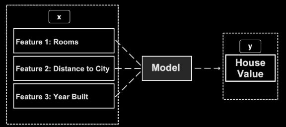
In machine learning, as in other statistical fields, dependent and independent variables are analyzed crosswise. Independent variable (x) is the input that affects the dependent variable (y) and dependent variable (y) is the output you wish to predict.
The goal of machine learning is to determine how independent variables (x) influence dependent variables (y).
As an example, supervised learning is a machine learning framework that uses independent variables (distance from city, number of bedrooms, land size, etc.) to predict the prices of houses in a neighborhood as the dependent variable. When inputting the features of a house (x), the prediction model can predict its value (y).
Three categories can be distinguished when it comes to self-learning:
Supervised learning
Unsupervised learning
Reinforcement learning
Supervised learning
In supervised learning, independent variables are decoded into dependent variables based on their known relationships. Various features (X) must be fed to the machine along with their known outputs (y). Datasets that are labeled have known input and output values, so the algorithm can decipher patterns in them and develop a model that interprets new data according to their underlying rules.
Unsupervised learning
Unsupervised learning relies on patterns among independent variables rather than knowing the dependent variables or labeling them. Using clustering analysis, similar data points can be grouped and connections can be found to generalize patterns, such as suburbs with two-bedroom apartments generating high property values. A dimensionality reduction algorithm uses unsupervised learning to create an output with fewer dimensions (features) than the original input.
An anomaly detection task, for example, is also popular among unsupervised learners.
Detecting manufacturing defects in fraudulent transactions
Preventing supervised learning algorithms from learning from complex datasets by automatically removing outliers
Reinforcement learning
Among the three categories of machine learning, reinforcement learning is the most advanced. When playing chess or driving an automobile, it is commonly used to make a series of decisions.
As opposed to unsupervised learning, reinforcement learning involves knowing the output (y) and unknown the inputs (X). By using a brute force technique based on trial and error, the optimal input is determined by comparing the output to the intended goal (e.g., winning a chess game). The model then grades random input data based on its relationship to the target output.
A self-driving vehicle, for example, grades movements that prevent a crash positively. Similar to chess, moves designed to avoid defeat are rewarded. By leveraging this feedback, the model gradually improves its choice of input variables to maximize output.
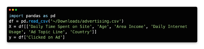
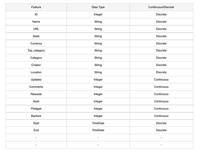
Introduction to Datasets
Among the attributes reported in this dataset are the gender, age, location, average daily online time, and whether the target advertisement was clicked.
Data on the Melbourne housing market
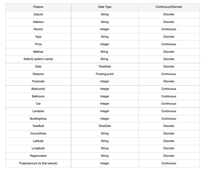
Melbourne, Australia, house, unit, and townhouse prices are included in this dataset. Data from publicly available real estate listings posted every week on the domain was scraped for this dataset. Twenty-one variables are included in this dataset, such as the address, suburb, land size, room count, price, longitude, latitude, and postcode.
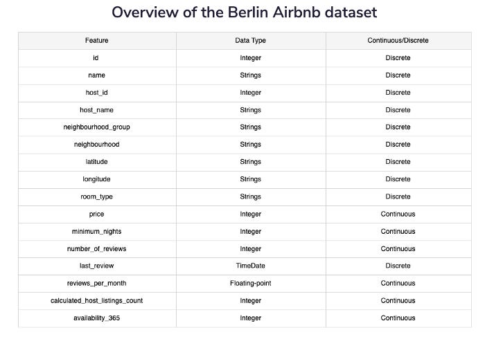
Berlin Airbnb data overview
Since Airbnb’s humble beginnings in 2008, its popularity has exploded. As of November 2018, Berlin had over 22,552 Airbnb listings, making it one of the largest markets in Europe for alternative accommodation. In addition to location, price, and reviews, the dataset contains detailed information.
Machine learning libraries: an introduction
There is rarely a single data scientist working alone. Therefore, it is essential to maintain consistent code so that other programmers can read it and reuse it. The use of code libraries is similar to the use of WordPress plugins for websites. Code libraries make it easy for data scientists to use prewritten modules of code to perform common tasks.
On a portfolio of websites, you can install a comment management plugin called Discuz. Developers do not have to become familiar with the underlying code for each website if they use the same plugin for all of them.
It is, however, necessary for them to become familiar with the Discuz plugin’s interface and customization settings.
As the same code interface can be used to access complex algorithms and other functions, machine learning libraries follow the same logic and benefits. Moreover, you can use a library like Scikit-learn to call a regression algorithm instead of writing the statistical requirements in many lines of code.

Pandas
Data management and presentation are made easy with Pandas. In Panda, it’s possible to create panels, similar to sheets in Excel, and this is where the name “Pandas” derives from. Like a spreadsheet or SQL table, Pandas can organize structured data as data frames, which are two-dimensional data structures.

NumPy
Python’s numeric language, NumPy, is often used in conjunction with Pandas. A number of mathematical functions are available using NumPy, including min, max, mean, standard deviation, and variance, as well as managing multi-dimensional arrays and matrices.
Using NumPy, you can process data with 50,000 rows or fewer in less memory and perform better than Pandas. A combination of NumPy and Pandas is often used in an interactive environment such as Jupyter Notebook because Pandas is more user-friendly.
NumPy arrays are designed to handle numerical data, particularly multidimensional data, while Pandas data frames are more suitable for managing a mix of data types.
Scikit-learn
General machine learning is based on Scikit-learn. In addition to shallow algorithms like logistic regression, decision trees, linear regression, gradient boosting, and more, it also offers a comprehensive repository of shallow algorithms. In addition to mean absolute error and data partition methods, such as split validation and cross-validation, it has a broad range of evaluation metrics.
Matplotlib
You can easily create scatterplots, histograms, pie charts, bar charts, error charts, and other visual charts using Matplotlib’s visualization library.
Seaborn
Using Matplotlib, Seaborn provides Python-based visualization. A variety of visual techniques are built into this library, including:
Independent and dependent variables visualized in color
Sophisticated heatmaps
Cluster maps
Pair-plots
It is easy to generate publication-quality visualizations with Seaborn’s preformatted visual design and Matplotlib’s customization capabilities. Charts and graphs are created directly from Pandas data-frames using the Plotly Python library (an interactive visualization Python library).
TensorFlow
It would be incomplete without mentioning TensorFlow, Google’s popular machine learning library. A wide range of shallow algorithms can be found in Scikit-learn, but TensorFlow is the library of choice for deep learning (DL) and artificial neural networks (ANNs).
In addition to allowing advanced distributed numerical computation techniques, TensorFlow was created at Google. By distributing computations over a network with thousands of GPU instances, TensorFlow supports advanced algorithms, including neural networks.
Due to the fact that Nvidia GPU cards are no longer included with macOS, TensorFlow is not compatible with Mac users. To access GPUs, Mac users must run their workloads in the cloud using TensorFlow.
An overview of exploratory data analysis (EDA)
EDA involves highlighting the salient characteristics of your dataset so that you can proceed to further analysis and processing.
A number of things need to be understood in order to perform EDA, including understanding the shape and distribution of the data, scanning for missing values, learning what features are most relevant for a given dataset, and understanding its overall contents. As a result of gathering this information, algorithms can be selected more effectively and areas of the data that need cleaning can be highlighted for subsequent processing.
Pandas provide a variety of simple tools for summarizing data, while Seaborn and Matplotlib provide additional options for visualization.
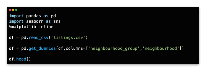
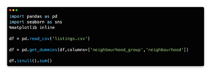
Here are the steps to import Pandas, Seaborn, and Matplotlib inline with Jupyter Notebook.

Importing the dataset
Datasets may be imported from internal as well as external files, and blobs may be generated randomly by users.
A Berlin Airbnb dataset was downloaded from Kaggle and used as a sample dataset. Detailed accommodation listings for Berlin were scraped from Airbnb, including location, price, and reviews.
Obtain the dataset by clicking the following link (after logging into Kaggle and creating a free account, download it as a zip file). As a Pandas data frame, import listings.csv into Jupyter Notebook using pd.read_csv after unzipping the downloaded file called listings.csv.

Depending on where you save the dataset and your computer’s operating system, the file path may vary. This example shows how to import a .csv file that was saved to the Desktop on Windows:

Backslashes are used in Python as escape characters, so you may need to prefix your pathname with r to indicate raw strings.

Data Frame Functions
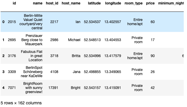
Jupyter Notebook now supports previewing data frames using Pandas head(). Data frame variable df must be called before head().

There is an index of zero at position 0 of the data frame for the first row (id 2015, located in Mitte). While the fifth row is indexed at position 4, the sixth row is indexed at position 1. When calling a specific row from a dataframe, you will need to subtract 1 from the actual number of rows because Python’s indexing starts at 0.
The columns of the data frame follow the same logic, even though they are not numerically labeled. A zero index is applied to the first column (id), and a four index is applied to the fifth column (neighbourhood_group). Whenever you call specific rows or columns, you need to keep in mind this fixed Python feature. When head() is called, the first five rows of the data frame are displayed by default. By specifying n rows inside the parentheses, you can increase the number of rows; you can see the results in the app below.
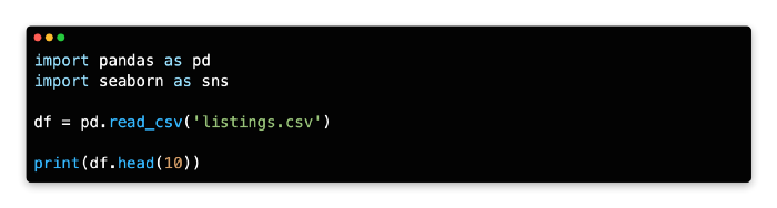
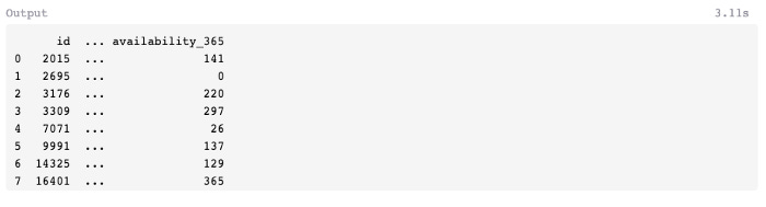
A preview of the data frame’s first ten rows is generated with the argument head(10). Scrolling to the right inside Jupyter Notebook will also reveal columns hidden to the right. A preview is only available for the number of rows specified in the code. Last but not least, n= is sometimes inserted inside head(), which is an alternative method to specify n rows to preview.
Example code:

Dataframe tail
Inversely, head() displays the top n rows of the data frame, while tail() displays the bottom n rows.
The following example shows a preview of the data frame using tail(), which shows five rows by default. The output will only be visible if you run the code.


Find row item
Despite their usefulness for understanding a data frame's basic structure, the head and tail commands are unsuitable for finding a single row or multiple rows in the middle of a large dataset.
Using the iloc[] method, you can retrieve a specific row or a sequence of rows from the data frame.

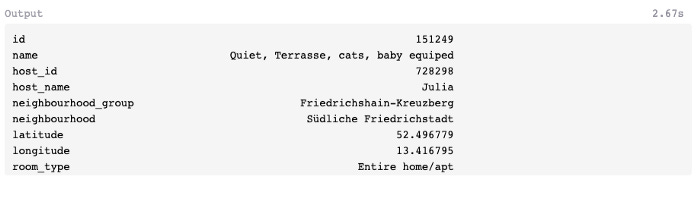
It retrieves row 151249 (a listing in the Friedrichshain-Kreuzberg neighborhood group) at position 99 in the dataframe, indexed at position 99 by df.iloc[99]. In case you require more detailed explanations of iloc, please refer to the provided link.
Shape
The shape method returns the number of rows and columns in the data frame, which can be used to quickly inspect the size of the data frame. By removing missing values, transforming features, and deleting features, you are likely to change the size of the dataset.
The shape method preceded by the dataset name can be used to query the number of rows and columns in the data frame (parentheses are not required).
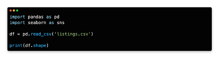

22552 rows and 16 columns make up this data frame.
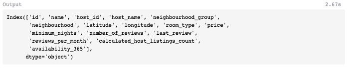
Columns
The columns method prints the titles of the columns in the data frame. If you need to copy and paste columns back into the code or clarify the names of specific variables, this is useful.

Describe
You can use describe() to summarize the mean, standard deviation, and interquartile range (IQR) values of a data frame. Optimal performance is achieved with continuous values. Numbers that can be aggregated easily, such as integers or floating-point numbers.

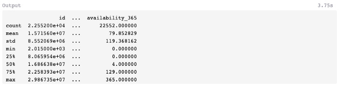
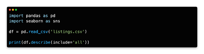
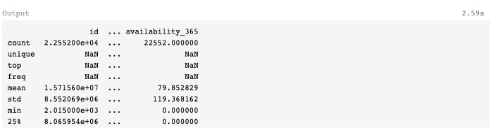
Columns with non-numeric values are excluded by default, and columns with numeric values are summarized statistically. The method can also be used to obtain a summary of both numeric and non-numerical columns (if applicable) by adding the argument include=’all’ within parentheses.
After covering Pandas methods for inspecting and querying the data frame size, let’s look at Seaborn and Matplotlib for generating visual summaries.
If you would like to learn more about Describe, you can click on the provided link.
Pairplots
Exploratory techniques such as pair plots are widely used to understand patterns between two variables. In a pair plot, variables are plotted against other variables from a data frame in a 2-D or 3-D grid. Below is an app that can provide you with such results.

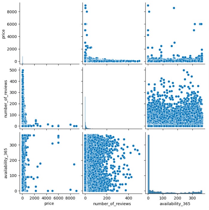
The pair plot from Seaborn allows you to compare three variables at the same time. As a result, we can better understand the relationships between the variables and their variances. The visualization takes the form of a scatterplot when plotted against other variables (multivariant), and a simple histogram when plotted against the same variable (univariant).
Introduction to Data Scrubbing
Why do we need to scrub data?
In the same way that a Swiss or Japanese watch runs smoothly and contains no extra parts, a good machine learning model should also. By avoiding syntax errors as well as redundant variables which can clog up the model’s decision path, the code can run smoothly.
As beginners code their first model, this bias towards simplicity is just as important. The creation of a minimal viable model is easier when working with a new algorithm, as it allows for complexity to be added later. If you find yourself at an impasse, look at the troublesome element and ask, “Do I need it?”
A model that cannot handle missing values or multiple variables types should be removed as soon as possible. As a result, the afflicted model should begin breathing normally again. Coding complexity can be added once the model is working.
Next, we will examine specific techniques for preparation, streamlining, and optimizing data.
Data scrubbing: what is it?
Scrubbing data is the process of manipulating it so that it can be analyzed.
Missing values or non-numeric input can result in error messages for some algorithms, for example. Data types may need to be converted or variables may need to be scaled.
Continuous variables can be analyzed using linear regression, for example. As an alternative, gradient boosting relies on integers or floating-point numbers to represent both discrete (categorical) and continuous variables.
Another problem often derailing a model’s ability to provide valuable insight is the presence of duplicate data, redundant variables, and errors in the data.
The removal of personal identifiers from data, especially private data, may also be considered when working with data, including private data. The problem is less of an issue when working with publicly available datasets, but should be considered when working with private data.
Data Scrubbing Operations
The following are data scrubbing operations:
Removing variables
One-hot encoding
Drop missing values
Dimension reduction
Data Scrubbing Operation: Removing Variables
Data preparation usually begins with removing variables that are not compatible with the selected algorithm or variables deemed less relevant to your target outcome. In general, exploratory data analysis and domain knowledge are used to determine which variables should be removed from the dataset.
As a starting point for exploratory data analysis, it is always helpful to check the variable types (strings, Booleans, integers, etc.) and correlations between them. By contrast, domain knowledge helps identify duplicate variables, such as country and country code, and eliminate less relevant ones, such as latitude and longitude.

Data Scrubbing Operation: One-Hot Encoding
It is not uncommon for data and algorithms to be mismatched or incompatible in data science. It is possible that the algorithm will not read the data in its default form even though the variable’s content might be relevant. Using general clustering and regression algorithms, for example, can’t parse and model text-based categorical values.
Changing categorical variables to numeric categorizers is one quick remedy. With one-hot encoding, categorical variables can be converted into binary values of “1” or “0” or “True” or “False” using a common technique called one-hot encoding.
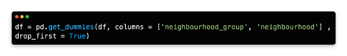
The dataframe expands horizontally when new columns are added using one-hot encoding. Even though expanding the dataset is not a major concern, using a parameter to remove expendable columns can simplify the dataframe and speed up processing. Each original variable is reduced by one column using the logic of deduction. Here is an example that illustrates this concept:
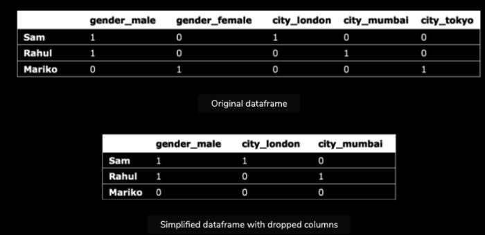
In spite of the fact that the expendable columns are missing from the second dataframe, the Python interpreter can still deduce each variable’s true value without reference to them. Based on the false arguments of city_london and city_mumbai, the Python interpreter can deduce that Mariko is from Tokyo. It describes the ability to predict a variable based on the value of another variable, which is known as multi-collinearity in statistics.
A parameter drop_first=True can be added to Python to remove expendable columns.
Data Scrubbing Operation: Drop Missing Values
The decision of what to do with missing data is another common but more complex problem. Three categories of missing data exist:
Missing completely at random (MCAR)
Missing at random (MAR)
Nonignorable.
The MCAR occurs when a missing value is not related to other values in the dataset. Datasets often do not contain values because they are not readily available.
MAR means that the missing value has no relationship with its own value, but has a relationship with other variables. For example, respondents in census surveys may skip an extended response question due to information they have already included in a previous question, or fail to complete an extended response question due to low levels of language proficiency stated elsewhere in the survey.
Consequently, the missing value is not directly related to the value itself but rather to another variable in the dataset.
Lastly, nonignorable missing data refers to data that is absent due to its own inherent value or importance. Respondents with a criminal record or those who have evaded taxes may opt not to answer a certain question because of sensitivity issues. Due to the fact that the data is missing, it’s difficult to diagnose why it’s missing.
The diagnosis and correction of missing values can be made easier with problem-solving skills and awareness of these three categories. For example, it might be necessary to reword surveys for second-language speakers in order to find non-ignorable missing values or redesign data collection methods, such as observing instead of asking for sensitive information directly from participants.
We can also manage and treat missing values more effectively if we have a decent understanding of why certain data is missing. Using the mean from existing data (of mostly male respondents) would be unnecessary in this case, as male participants are more likely to provide information about their salary than female participants.
Because MCARs are based on a random sample, they are relatively simple to manage and aggregate. Throughout this chapter, we’ll discuss common methods for filling missing values, but first let’s look at how to inspect missing values in Python.
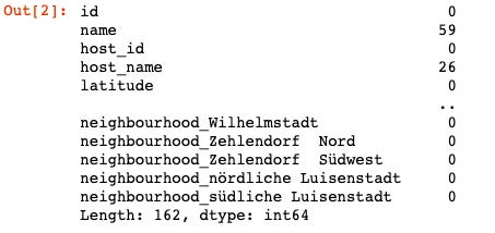
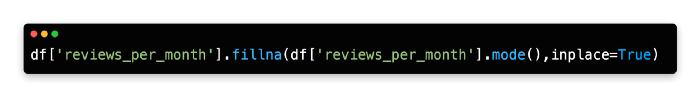
Using this method, you can gain a general idea of which features are missing values. It is evident from this table that four variables contain missing values, most notably last_review (3908) and reviews_per_month (3914). In addition to filling these missing values with several options, they will not be required for use with all algorithms. To fill in missing values, use the fill.na method to find the average value for the variable.

By replacing the missing values for the variable reviews_per_month with its mean (average), which in this example is 1.135525, the code replaces the missing values for the variable reviews_per_month.
We cannot use a reliable mode value in this dataset since the mode value is NAN. This often happens when floating-point numbers are used instead of integers (whole numbers). In parentheses, you can specify a custom value to fill missing values, such as 0.

If there are a lot of missing values in a row or column, the analysis can be discarded. In the absence of reliable stop-gap solutions, the mean, mode, and artificial values must be removed. You should also remove values if a variable is not central to your analysis or if there are a small number of missing values.
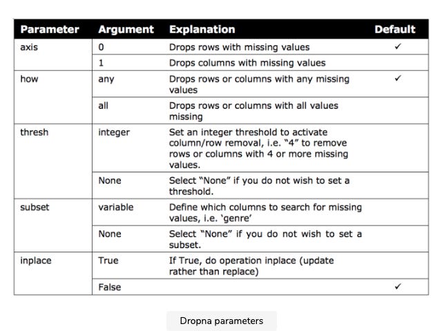
Missing values can be removed using two primary methods. In the first method, missing values are removed manually with the del function. Dropna (demonstrated below) eliminates missing values on an individual basis from columns or rows based on their contents.
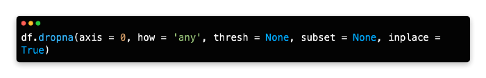
The best way to maintain more original data in a dataset is to drop rows rather than columns since datasets typically have more rows than columns. In the following table, the parameters for this technique are explained in detail.
As a result, handling missing values is not always straightforward, and your response will often depend on the type of data and the frequency of missing values. As an example, the variables last_review and reviews_per_month have many missing values, so they should be removed from the Berlin Airbnb dataset.
As these values are expressed numerically and can be aggregated easily, you could use the mean to fill reviews_per_month. In contrast to integers and floating-point numbers, last_review is expressed as a timestamp and can’t be aggregated.
It is also problematic to fill in artificial values for the other variables containing missing values, name and host_name. Due to their discrete nature, these two variables cannot be estimated using the mean and mode. Considering how few missing values these two variables have, they might be removed row-by-row.
Data Scrubbing Operation: Dimension Reduction
Data is transformed to a lower dimension using dimension reduction, also known as descending dimension algorithms. In this way, computational resources can be reduced and patterns in the data can be visualized.
Data dimensions are variables that describe the data, such as the city of residence, the country of residence, the age, and the gender. It is easier for the human eye to interpret three-dimensional and two-dimensional plots than four-dimensional plots.
In descending dimension algorithms, the goal is to produce a set of variables that mimic the original dataset’s distribution. By reducing the variables, patterns, such as outliers, anomalies, and natural groupings, can be identified more easily.
A dimension reduction doesn’t involve deleting columns, but rather mathematically transforming the data in those columns so that fewer variables (columns) are required to capture the same information. A study of house prices, for example, may reveal multiple correlated variables (such as house area and postcode) that could be combined into one variable that represents them both adequately. The model will run faster, consume less computing resources, and may provide more accurate predictions when dimension reduction is applied before the core algorithm.
Multidimensional data can also be visualized using this technique. For a scatterplot, four dimensions are the maximum number of dimensions that can be plotted. A scatterplot can be used to project synthetic variables onto the visual workspace of a scatterplot even if two or three dimensions (the fourth is time) are best.
Scatterplots are useful both for explaining and exploring patterns and relationships. When the analysis is in progress, exploratory graphics are usually generated on the fly to assist internal understanding. A post-analysis audience receives explanation graphics.
A multidimensional dataset can be streamlined into four or fewer variables (suitable for scatterplots), but it’s not necessary for machine learning. Scatterplots cannot display the output from models that examine the input of, say, 20 variables, but the models can still produce binary output such as 1 (True) and 0 (False) or another form of output based on the input.
Pre-Model Algorithms
In this part, I will introduce you to the pre-model algorithm and describe how principal component analysis is implemented (1–3).
The pre-model algorithm in a nutshell
To prepare data for prediction modeling, unsupervised learning algorithms are sometimes used as an extension of the data scrubbing process. Instead of providing actionable insight into the data, unsupervised algorithms clean or reshape it.
As discussed in the previous chapter, dimension reduction techniques and k-means clustering are examples of pre-model algorithms. In this chapter, we examine both algorithms.
PCA
In dimension reduction, PCA is one of the most popular techniques. It reduces data complexity dramatically and makes data easier to visualize in fewer dimensions by using general factor analysis.
A PCA aims to minimize the number of variables in the dataset while preserving as much information as possible. The PCA method recreates dimensions by combining features into linear combinations called components rather than removing individual features. You can then drop components that have little impact on data variability by ranking those that contribute the most to patterns in the data.
PCA aims to maximize variance along the first axis by placing the axis in the direction of the greatest variance of the data points. In order to create the first two components, a second axis is placed perpendicular to the first axis.
According to the position of the first axis, the second axis is positioned in a two-dimensional setting. When the second axis is perpendicular to the first axis in a three-dimensional space, it’s important to position it so it maximizes the variance on its axis. The following figure illustrates PCA in a two-dimensional space.
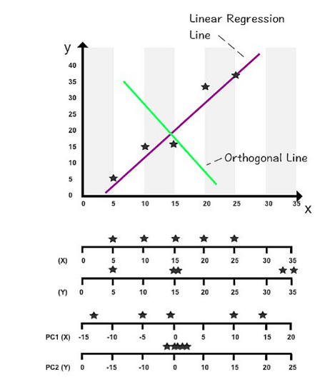
A horizontal axis is shown above. X and Y values are measured on the first two axes. X and Y values are measured by the second two axes when rotated 90 degrees. By using the orthogonal line as an artificial y-axis, it is possible to visualize the rotated axes. The linear regression line takes on the role of the x-axis in the following figure.
The first two components of this dataset can be found on these two new axes. The PC1 axis and PC2 axis are the new axes.
You can see a new range of variance among the data points by using PC1 and PC2 values (depicted on the third and fourth axes). On the first axis, PC1’s variance has increased compared to its original x values. As all the data points are close to zero and virtually stacked on top of each other, the variance in PC2 has shrunk significantly.
You can concentrate on studying PC1’s variance since PC2 contributes the least to overall variance. Despite not containing 100% of the original information, PC1 captures the variables that most impact data patterns while also minimizing computation time.
Before selecting one principal component, we divided the dataset into two components. Another option is to select two or three principal components that contain 75% of the original data out of a total of ten components. The purpose of data reduction and maximizing performance would be defeated if we insisted on 100% of the information. There is no well-accepted method for determining how many principal components are needed to represent data optimally. The number of components to analyze is a subjective decision based on the dataset size and the extent to which the data needs to be shrunk.
You will reduce a dataset to its two principal components in this coding exercise. In this exercise, we will use the Advertising Dataset.
1: Import Libraries
NumPy, Pandas, Seaborn, Matplotlib Pyplot, and Matplotlib inline are a few Python libraries we will need to import first. In a Jupyter notebook, enter the following code to import each library.
2: Import Datasets
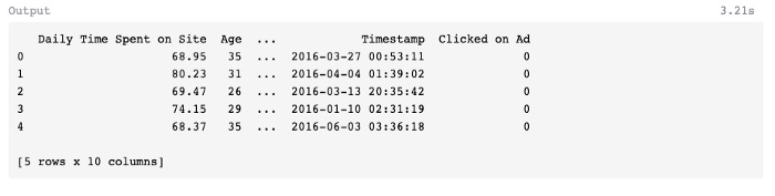
In the next step, the dataset will be imported into the same cell. Once you log in to Kaggle, you can download the Advertising Dataset as a zip file. After downloading the CSV file, unzip it and import it into Jupyter Notebook using pd.read_csv() and adding the path for the file directory.
Using this command, a Pandas data frame will be created from the dataset. From the top menu, select “Cell” > “Run All” to review the data frame or use the head() command and click “Run.”
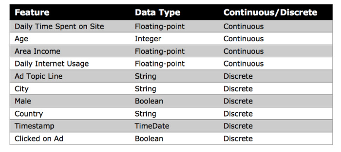
A few of the features of this dataset are shown below, including Daily Time Spent on Site, Age, Area Income, Daily Internet Usage, Ad Topic Line, City, Male, Country, Timestamp, and Clicked on Ad.

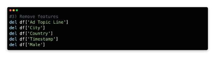
3: Remove Features
This algorithm cannot parse non-numerical features, such as Ad Topic Line, City, Country, and Timestamp, so you must remove them. Although Timestamp values are expressed in numbers, their special formatting makes it impossible to use this method to calculate mathematical relationships between variables.
Our model only examines continuous input features, so you need to remove the discrete variable Male, expressed as an integer (0 or 1).
We’ll remove these five features using the del function and the columns we’d like to remove using the remove function.
PCA Implementation Steps: 4 to 6
Scale Data
StandardScaler standardizes features by scaling to unit variance and assuming zero as the mean for all variables in Scikit-learn. A data frame with transformed values is created based on the mean and standard deviation that are then stored and used later with the transform method.
When StandardScaler has been imported, it can be assigned as a new variable, adapted to the data frame’s features, and transformed.
Data features are rescaled and standardized using StandardScaler in combination with PCA and other algorithms, such as k-nearest neighbors and support vector machines. A dataset can, for example, adopt the properties of a normal distribution when these two parameters are combined.
In the absence of standardization, the PCA algorithm will likely focus on features that maximize variance. The effect may be exaggerated by another factor, however. As you measure Age in days rather than years, you will notice that the variance changes dramatically. Left unchecked, this type of formatting could mislead a selection process that maximizes variance in selecting components. The StandardScaler rescales and standardizes variables to avoid this problem.
The scale of the variables may not require standardization if they are relevant to your analysis or consistent.

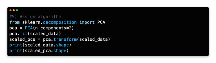
5: Assign Algorithm
The PCA algorithm can now be imported from Scikit-learn’s decomposition library after we’ve laid the groundwork.
Please pay attention to the next line of code, as it reshapes the features of the data frame into components. You will need to identify the components that have the greatest impact on data variability for this exercise. Choosing two components (n_components=2) instructs PCA to find the two components best explaining the data variability. Depending on your needs, you can modify the number of components, but two components are the easiest to interpret and visualize.
With the transform method, you can recreate the data frame’s values using the two components fitted to the scaled data.
To compare the two datasets, let’s use the shape command to check the transformation.
The scaled PCA data frame can now be queried for its shape.
As you can see, the PCA has compressed the scaled data frame from 1,000 rows and 5 columns to 1,000 rows and 2 columns.
6: Visualize the Plot
We can visualize the two principal components on a two-dimensional scatterplot using the Python plotting library Matplotlib, with principal component 1 marked on the x-axis and principal component 2 marked on the y-axis. In the first version of the code, you will visualize the two principal components without a color legend.
Plot 1:
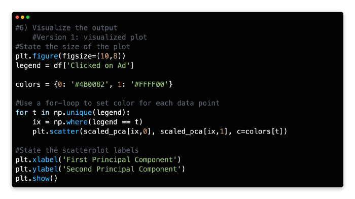
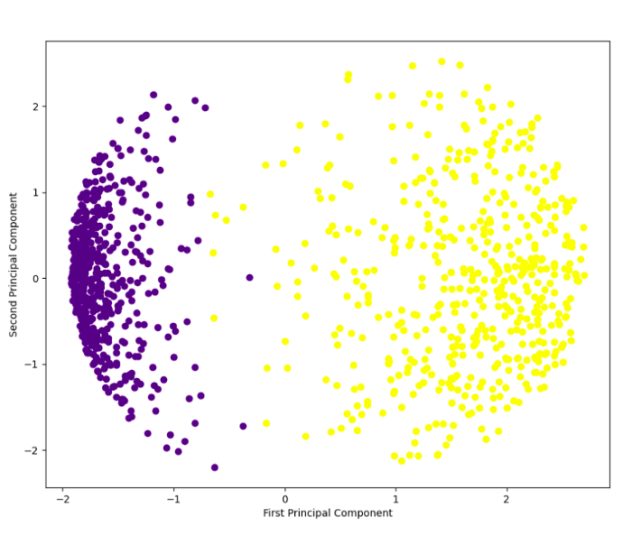
Each component is color-coded to indicate whether the user clicked on the ad or did not click on it. Rather than representing a single variable, components represent a combination of variables.
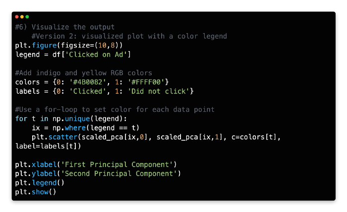
A color legend can also be added to the code. Rapidtables provides RGB color codes and Python for-loops for this more advanced set of code.
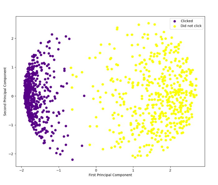
With the help of a color legend in the top right corner, you can clearly see the separation of outcomes. With PCA output in hand, supervised learning techniques like logistic regression or k-nearest neighbors can be used to further analyze the data.
K-Means Clustering Implementation Steps: 1 to 3
K-means clustering is another method for reducing data complexity by identifying groups of data points without knowing the class of the data.
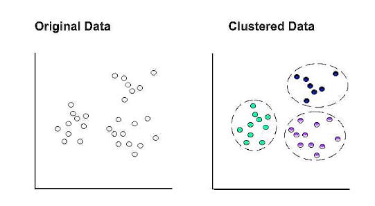
In K-means clustering, k represents the number of clusters within the dataset. For example, setting k to “3” separates the data into three clusters.
A cluster’s centroid becomes the epicenter when a data point is assigned to it at random. Those points that do not have a centroid are assigned to the closest centroid. A new cluster’s mean is used to update the centroid coordinates. A new cluster may be formed based on comparative proximity with a different centroid as a result of this update. It is then necessary to recalculate and update the centroid coordinates.
In the final set of clusters, all data points remain within the same cluster after the centroid coordinates are updated.
Exercise
The purpose of this exercise is to create an artificial dataset and use k-means clustering to divide the data into four natural groups.
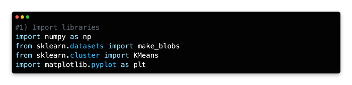
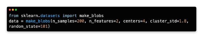
1: Import libraries
Scikit-learn’s make_blobs algorithm was used to generate the artificial dataset for this exercise. A Matplotlib Pyplot and Matplotlib inline visualization will be created for this exercise.
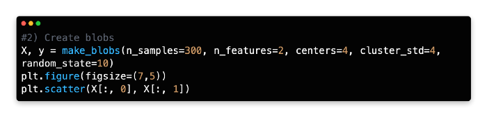
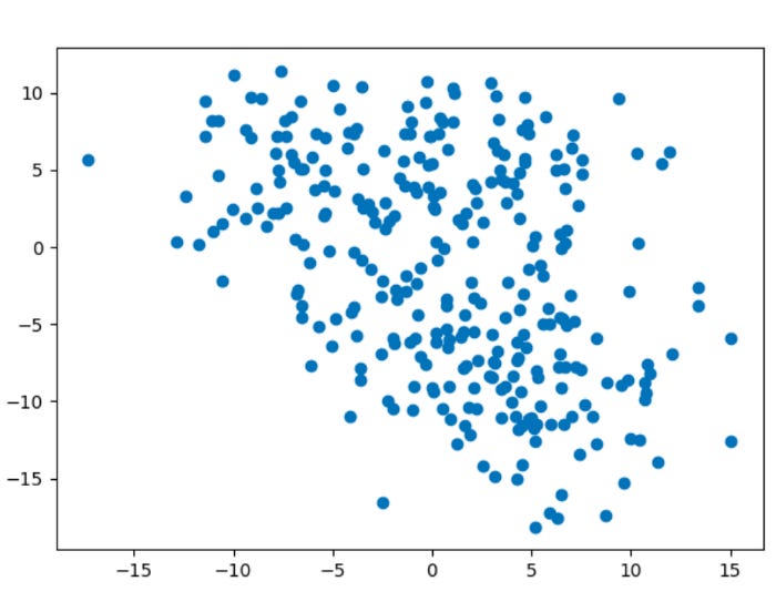
2: Create Blobs
As an alternative to importing a dataset, we generated an artificial dataset with 300 samples, 2 features, and four centers, with a cluster standard deviation of 4.
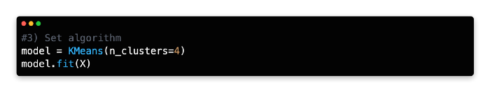
3: Set Algorithm
To discover groups of data points with similar attributes, you want to use k-means clustering. Before fitting the model to the artificial data (X), create a new variable (model) and call the KMeans algorithm from Scikit-learn.
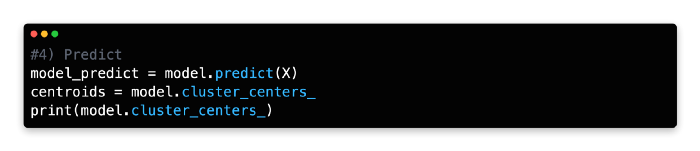
4: Predict
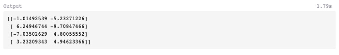
You can run the model and generate the centroid coordinates using cluster_centers by using the predict function under the new variable (model_predict).
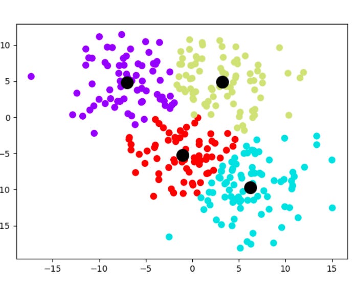
5: Visualise the Output
The clusters will now be plotted using two sets of elements on a scatterplot. Under the variable named model_predict, you will find four color-coded clusters produced by the k-means model. A second variable, centroids, stores the cluster centroids.
There are black centroids with marker sizes of 200 and alphas of 1. It can take any float number between 0 and 1.0, where 0 represents maximum transparency and 1 represents maximum opaqueness. You need the alpha to be 1 (opaque) since you are superimposing the four cluster centroids over them.
You can find more information about the scatterplot features in Matplotlib here.
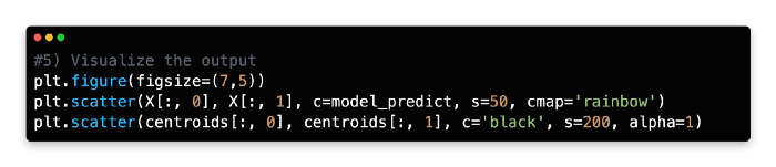
The k-means clustering method has enabled you to identify four previously unknown groupings within our dataset and streamline 300 data points into four centroids for generalization.
In the previous chapter, we discussed k-means clustering as a method to reduce a very large dataset into manageable cluster centroids for supervised learning.
A supervised learning technique or another unsupervised learning technique may be used to further analyze the data points within each cluster. One of the identified clusters may even benefit from k-means clustering, which is useful for tasks such as identifying customer subsets in market research.
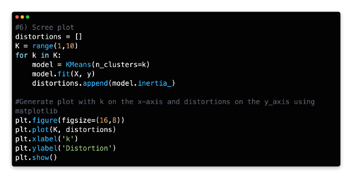
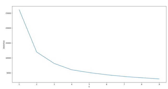
6: Scree Plot
Consider analyzing a scree plot for guidance when optimizing k. Scree plots illustrate scattering (variance) by comparing the distortion between different cluster variations. Based on the Euclidean distance between the centroid and the other points in a cluster, distortion is calculated as the average of the squared distance between those points.
In order to determine the optimal number of clusters, one must determine the value of k where distortion gradually subsides on the left side of the scree plot, without reaching a point where cluster variations are negligible on the right. From the optimal data point (the “elbow”), distortion should decrease linearly to the right.
For our model, 3 or 4 clusters appear to be the optimal number. Due to a pronounced drop-off in distortion, these two cluster combinations have a significant kink to the left.
The right side of the graph also exhibits a linear decline, especially for k = 4. As the dataset was generated artificially with 4 centers, this makes sense.
Using Python, you can calculate the distortion values for each k value by iterating through the values of k from 1 to 10. To plot the screen plot, Python and Matplotlib must be used with the for loop function.
Find distortion values for each value of k using a for loop with a range of 1–10.
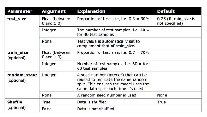
Split Validation
A technique called split validation is crucial to machine learning, as it allows the data to be partitioned into two distinct sets.
In order to develop a prediction model, the first set of data is called the training data.
Testing the model’s accuracy from the training data is done using the second set of data.
In most cases, the training data is larger than the test data by 70/30 or 80/20. The model is ready to generate predictions using new input data once it has been optimized and validated.
Models are built from the training data only, even though they are used on both training and test sets.
Models are created using test data as input, but they should never be decoded or used to make predictions. The validation set is sometimes used by data scientists because the test data cannot be used to build and optimize the model.
Using the validation set as feedback, the prediction model can optimize its hyperparameters after building an initial model based on the training set. Afterward, the prediction error of the final model is assessed using the test set.
Validation and test data can be reused as training data to maximize data utility. In order to optimize the model just before it is used, used data would be bundled with the original training data.
Train and test set
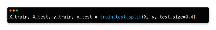
Python’s train_test_split library requires an initial import of sklearn.model_selection in order to perform split validation.

The x and y values need to be set before using this code library.

A random seed of 10 is ‘bookmarked’ for future code replication so that the training/test data is split 70/30 and shuffled.
Train Test Split can be explained in more detail by following the provided link.
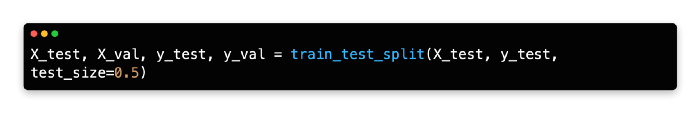
Validation set
In the current version of Scikit-learn, there is no function to create a three-way split between train/validation/test.
As demonstrated below, one quick solution is to split the test data into two partitions.
Data for training is set to 60%, while data for testing is set to 40%. A 50/50 split is then performed so that the test data and validation set represent 20% of the original data each.

Introduction To Model Design
It’s helpful to take a step back and look at the entire process of building a machine learning model before diving into specific supervised learning algorithms. Several steps discussed in previous chapters will be reviewed and new methods will be introduced, such as evaluating and predicting.
The 10 steps follow a relatively fixed sequence inside your development environment. From start to finish, you will find it easy to design your own machine learning models with this framework.
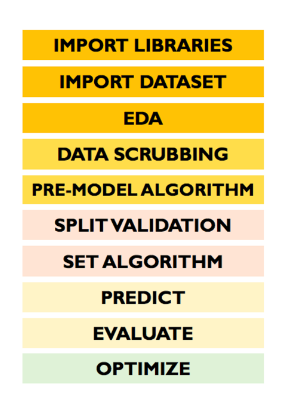
The following steps are involved in the model design:
Import libraries
Import dataset
Exploratory data analysis
Data scrubbing
Pre-model algorithm
Split validation
Set algorithm
Predict
Evaluate
Optimize
Import Libraries
It’s crucial to import libraries before calling any specific functions in Python, since the interpreter works from top to bottom. Using Python without Seaborn and Matplolib will not allow you to create a heatmap or pair plot, for example.
Your notebook doesn’t have to have the libraries at the top. When importing algorithms-based libraries, some data scientists prefer to import them before references to them in code sections where they are used.
Import Datasets
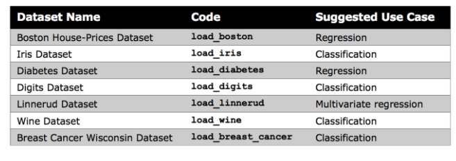
Kaggle or your organization’s records are generally used to import datasets. Kaggle offers a wide selection of datasets, but Scikit-learn provides several small built-in datasets that don’t require external downloads.
For beginners, these datasets are useful for understanding new algorithms, as noted by Scikit-learn. In your notebook, you can directly import Scikit-learn’s datasets.

Make Blobs
The k-means clustering lesson uses Scikit-learn’s make blobs function to generate a random dataset. Rather than offering meaningful insights, this data can help gain confidence in a new algorithm.

Exploratory Data Analysis
As a result of the third step, EDA, you will gain a better understanding of your data, including the distribution and the status of missing values. During exploratory data analysis, you also determine which algorithm to use for data scrubbing.
The EDA may also come into play during the process of checking the size and structure of your dataset and integrating that feedback into model optimization.
Data Scrubbing
Developing a prediction model usually requires the most time and effort during the data cleaning stage. It’s essential to pay attention to the quality and composition of your data, just like you would with a good pair of dress shoes.
Clean up the data, inspect its value, repair it, and, ultimately, decide when to discard it.
Pre Model Algorithm
In preparation for analyzing large and complex datasets, unsupervised learning techniques, such as k-means clustering analysis and descending dimension algorithms, may be applied as an extension of the data scrubbing process.
Prior to conducting further analysis with supervised learning, k-means clustering reduces row volume by compressing rows into fewer clusters based on similar values.
Nevertheless, this step is optional, especially when working with small datasets with a limited number of dimensions (features).
Split Validation
Data is partitioned for training and testing analysis using split validation. If you want to replicate the model’s output in the future, it is useful to randomize your data at this point using the shuffle feature.
Set Algorithm
Every machine learning model begins with the algorithm, which must be carefully chosen.
Algorithms are mathematically based sequences of steps that react to changing patterns to generate output or decisions. In order to interpret patterns, make calculations, and reach decisions, the model executes a series of steps defined by the algorithm.
As input data varies, algorithms can produce a variety of outputs depending on it. Also, algorithms can be customized by adjusting hyperparameters to create a more customized model.
In this sense, algorithms are more like moving frameworks than concrete equations, and they can be customized based on the output the algorithm is meant to produce and the input data it is used with.
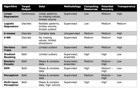
It is important not to confuse the algorithm with the model for context. A model is the result of combining hyperparameters that have been adjusted based on the data and combining data scrubbing, split validation, and evaluation techniques. The following is a list of common characteristics of popular machine learning algorithms.
Predict
For validation, the predict function is called on the test data after the initial model has been developed using the training data.
Predict functions generate numeric values, such as prices or correlation indicators, for regression problems. The predict function creates discrete classes, such as movie categories and spam/non-spam categories.
Evaluate
Following the design of the model, the results are evaluated. Depending on the scope of your model, you will need to use a different evaluation method. A classification or regression model will have a different response depending on its type. An accuracy score, a confusion matrix, and a classification report are all common methods for evaluating classification.
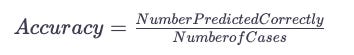
Accuracy Score
Based on the total number of cases, this metric measures how many cases were classified correctly. A score of 1.0 indicates that all cases were correctly predicted, whereas a score of 0 indicates that all cases were incorrectly predicted.
A high number of false positives or negatives may be hidden by accuracy alone, which is normally a reliable performance metric. Having a balanced number of false positives and false negatives isn’t an issue, but it’s also something you can’t determine based solely on accuracy. The following two evaluation methods are therefore considered.
Confusion Matrix
Confidence matrices (also called error matrices) summarize a model’s performance, including all the false positives and false negatives.
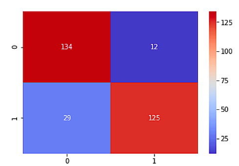
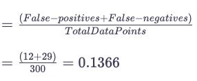
The model in this example correctly predicted 134 data points as “0” and 125 cases as “1”, as shown in the top left box. A total of 12 data points were predicted as “1” and 29 as “0” by the model. In other words, the 12 data points on which a false-positive prediction was made should have been classified as (0), and the 29 data points on which a false-negative prediction was made should be numbered (1).
Calculate the accuracy of the predictions using the confusion matrix by dividing the total number of false-positives (12) and false-negatives (29) by the total number of data points, which is 300 in this case.
Classification Report
Classification reports, which generate three evaluation metrics and support information, are another popular evaluation technique.
Precision
Predicting true positives as a percentage of all predicted positives is known as precision. False positives are unlikely to occur when precision scores are high.

A model’s accuracy in predicting a positive outcome is measured with this metric. As a result, a negative case is not labeled as a positive case, which is important for drug tests.
Recall
Similarly to precision, recall shows the ratio of correctly predicted to actually observed true positives in a model. Basically, recall measures the number of positive outcomes that were classified correctly. All positive cases can be identified by the model if it is capable of doing so. Both precision and recall have the same numerator (top), but their denominators (below) differ.

F1 Score
Precision and recall are combined to calculate the F1-score. Rather than serving as a stand-alone metric, it’s typically used to compare models.
Because recall and precision are calculated differently, the f1-score is generally lower than the accuracy score.
Optimization
Last but not least, the model must be optimized. Changing the hyperparameters of a tree-based learning technique for clustering analysis may require modifying the number of clusters.
A trial and error system can be used to optimize models manually, or grid search can be used to automate the process.
By using this technique, you can test a range of possible hyperparameters and methodically test each one. The optimal model is then determined by an automated voting process.
In line with how many combinations you set for each hyperparameter, grid search can take a long time.
Linear And Logistic Regression
Implementation of Linear Regression And Logistic Regression
Linear regression: a quick overview
As you may know, linear regression is a process that plots a straight line or plane called the hyperplane to predict a data set’s target value by identifying the relationship between a variable’s dependent and independent variables. Hyperplanes are subspaces that correspond to p*1 dimensions in p-dimensional space
Hyperplanes are one-dimensional subspaces/flat lines in two-dimensional spaces. Hyperplanes are effectively two-dimensional subspaces in three-dimensional space. Despite the difficulty of visualizing a hyperplane with more than one dimension, a p*1 hyperplane still exists.
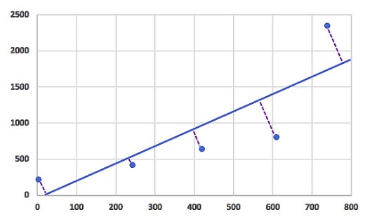
By bisecting the known data points, the hyperplane aims to minimize the distance between itself and each data point. A perpendicular line drawn from the hyperplane to every point on the plot will be the smallest distance for any potential hyperplane if a perpendicular line is drawn from it to every point on the plot.
Building a linear regression model begins with removing or filling out missing values and confirming the dependent variable’s most correlated independent variables. Correlations between independent variables should not exist, however.
It is called collinearity (if two variables are correlated) or multicollinearity (if more than two variables are correlated) if individual variables do not have unique values as a result of strong linear correlation between them.
The model is not affected by this, but it affects the individual (independent) variables’ calculations and interpretations. The output (dependent variable) can still be predicted reliably using collinear variables. When it comes to determining the model’s output, it is difficult to distinguish between variables that are influential and those that are redundant.
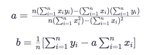
The Linear Regression Equation
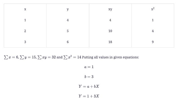
Here is the equation: Y=a + bXY=a+bX, where Y is the dependent variable, X is the independent variable, b is the slope of the line, and a is the y-intercept.
Example
Given set of points {(1,4), (2,5), (3,6)}
The Following Steps are involved in the implementation of LR:
Import libraries
Import dataset
Remove variables
Remove or modify variables with missing values
Set x and y variables
Set algorithm
Find y-intercept and x coefficients
Predict
Evaluate
Exercise
Using four independent variables, you will code a linear regression model to predict house prices. A prediction of the dependent variable (price) can be made by adding the correlation coefficients of each independent variable to the y-intercept. For this model, we scraped real estate listings from Melbourne, Australia, and used the Melbourne Housing Dataset. There are 21 variables in the data set: the address, the suburb, the land size, the number of rooms, the price, the longitude, the latitude, and the postcode.
Linear Regression Implementation
1: Import Libraries
The following Python libraries need to be imported first:

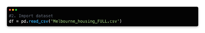
2: Import Dataset
Assign the data frame df as a variable using the equals operator using Pandas pd.read_csv command.
There are some spelling errors in this dataset, but this will not affect our code, as we will remove these two variables in Step 3.
3: Remove Variables
There are two ways to develop regression models. A limited number of variables can explain a large proportion of the variance by following the principle of parsimony. To capture maximum variance, more variables are used, including variables that explain a small proportion of variance.
With the addition of computational resources and model complexity, both methods have pros and cons.
Due to convenience, we will only use a few variables in our model. The model will also include variables that already have numerical expressions, including Price, Distance, BuildingArea, Bedroom2, Bathroom, Rooms, Car, Propertycount, and Landsize. The algorithm can read non-numerical variables such as Address, Method, SellerG, Date, etc., without transforming them into a numerical format.
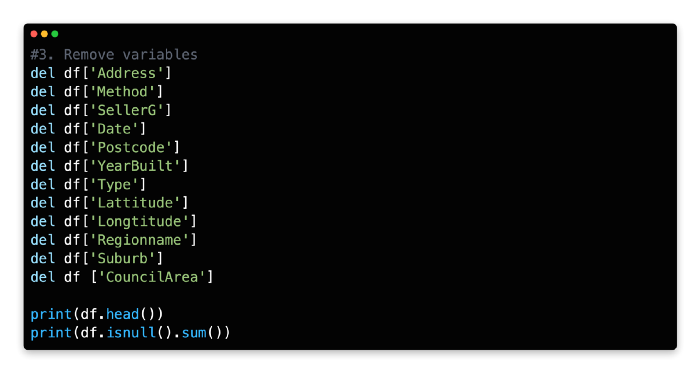

More than half of the variables in the original dataframe have been removed, as can be seen in the output above. NaN (not a number) is also common among real-life datasets, which indicates a high number of missing values. The isnull().sum() function can be used to inspect the full extent of missing values.
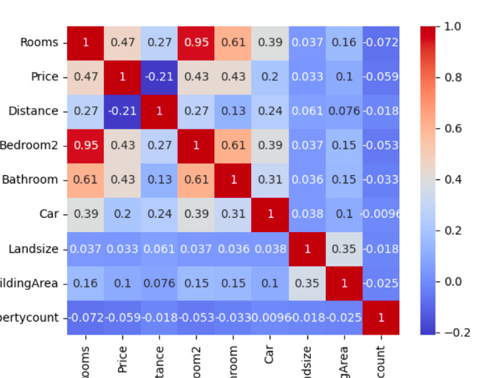
A total of 21,115 missing values are recorded in BuildingArea, ranging from 1 (Distance). In the next section, we’ll address how to deal with these missing values. As a last step, let’s use a heatmap to analyze the correlation (corr) between all combinations of variables.
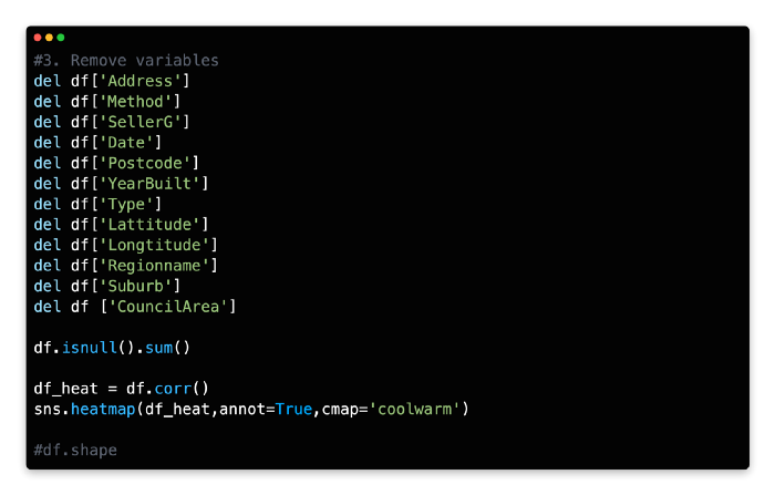
Last but not least, let’s examine the dataset’s shape.
Based on the output of df.shape, there are 34,857 rows and 9 columns (features) in the data frame.
There is a high correlation between Bedroom2 and Rooms (0.95). A strong correlation between independent variables should be avoided, as mentioned earlier. As a result, one of these variables will need to be removed.
It is up to you to choose which variable to remove based on the information you wish to gain from our model. As Bedroom2 (the second bedroom) is more narrowly defined than Rooms, it may be useful. An extra bedroom could be added to the property with this explicit knowledge, for example. Nevertheless, we will include the variable Rooms in our model and remove the variable Bedroom2 because there are no missing values for Rooms.
Our linear regression model will also be hampered by the removal of Landsize (0.033) and Propertycount (0.059), as these variables show low correlation to the dependent variable Price.

4: Remove or Modify Variables With Missing Values
This dataset has missing values, which may pose a problem for linear regression, particularly because of its missing values. The data frame must therefore be estimated or removed from these values.
Nevertheless, removing all missing values on a row-by-row basis will greatly reduce the size of the data frame. There are 21,115 missing rows in the variable BuildingArea, which represents two thirds of the data frame! Due to its low correlation with the dependent variable of Price (0.1), you can remove this variable entirely.
A row-by-row removal can be done or the mean value can be filled in for the remaining variables. The following can be done based on exploratory data analysis:
For variables with partial correlation to Price (e.g., Car), use the mean.
In the case of variables with a small number of missing values (such as Distance), remove the rows.
Replace missing values row-by-row with those that have a significant correlation to Price (for example, Bathroom).
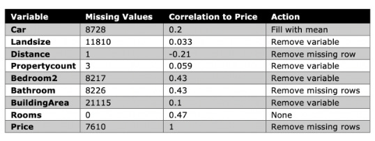
When most variables have missing rows, the default setting is to remove the missing rows, rather than to remove the entire variable or artificially fill the rows with the mean.
Unless you remove all the variables containing missing values, most of the missing values appear in the same recurring rows. Let’s fill or remove the missing values in our model next to continue building it.

Following the removal of BuildingArea and filling in the missing values for Car, it is important to drop the missing rows.
Now let’s examine how many rows remain in the data frame.
df.shape
##Output: (20800, 8)
Our linear regression model can be built with 20,800 rows, just over half of the original dataset.
5: Set X and Y Variables
The next step is to assign our variables X and Y. In the X array, you have independent variables, and in the Y array, you have the dependent variable (Price).

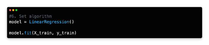
6: Set Algorithm
Using the equals operator, assign the linear regression algorithm from Scikit-learn as a variable (i.e., model or linear_reg). It doesn’t matter what the variable is named as long as it’s an intuitive description and follows the Python syntax for assigning variables (no spaces, no numbers, etc.).
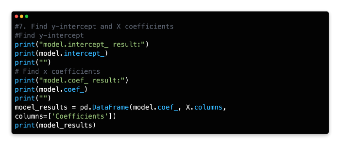
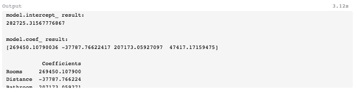
7: Find y-intercept and X Coefficient
Our model’s y-intercept and coefficients for each independent variable can be viewed using the following code. To view the output of each function, you will need to run them separately (remove one function from the model and run the other).
8: Predict
The model can now be run to find the value of an individual property by creating a new variable (new_house) and incorporating the following inputs:
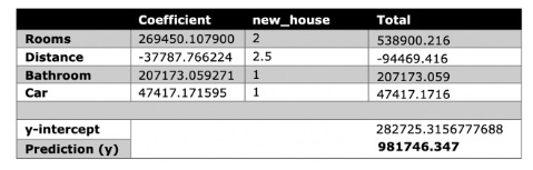


This house is predicted to be worth AUD $981,746.347. AUD $1,480,00 is the actual value of the house, based on the dataset.
9: Evaluate
Next, you can compare the actual price against the model’s predicted price using mean absolute error from Scikit-learn.
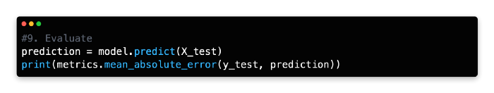

According to the model, the price of the actual listing was miscalculated by approximately $363,782 on average, which means that the model averaged 363782.9423236326, or 363782.942323632.
Since 16 variables were removed from the original dataset, this relatively high error rate is not surprising. As an example, the Type (house, apartment, or unit) variable plays an important role in determining house value. We did not include this variable in our model since it is expressed non-numerically. The model could be reconstructed using one-hot encoding and Type could be converted into numeric variables.
Linear regression is extremely fast to run, but its prediction accuracy is not well known. There are, however, more reliable algorithms available, which we will discuss in the following chapters.
For more information about linear regression, Scikit-learn provides detailed documentation, including a practical code example. As described in this chapter, the documentation does not demonstrate split validation (training and test splits) for linear regression.
Implementation Of Logistic Regression
As a general rule, machine learning involves predicting a quantitative or qualitative outcome. Regression problems are commonly referred to as the former. With linear regression, continuous variables are used to predict a numeric outcome.
Classification problems involve predicting qualitative outcomes (class). Predicting what products a user will buy or whether an online advertisement will be clicked are examples of classification problems.
The logistic regression algorithm, for example, does not neatly fit into this dichotomy. A logistic regression is part of the regression family since it uses quantitative relationships between variables to predict outcomes. While linear regression accepts only continuous variables as input, qualitative regression accepts both continuous and discrete variables. Moreover, it predicts discrete classes such as “Yes/No” or “Customer/Non-customer”.
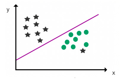
Analyzing relationships between variables is the purpose of the logistic regression algorithm. Sigmoid functions are used to assign probabilities to discrete outcomes, converting numerical results into a probability expression.
A probability of 1 is greater than 0, whereas a probability of 0 is much lower. Binary predictions can be classified into two discrete classes based on the cut-off point of 0.5. The class A predictions are those above 0.5, and the class B predictions are those below 0.5.
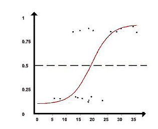
A hyperplane is used as a decision boundary to split the two classes (to the best of its ability) after assigning data points to a class with the Sigmoid function. It is then possible to predict the class of future data points based on the decision boundary.
The Logistic Regression Question
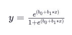
Y is the expected output, b_0b0 represents the bias or intercept term, and b_1b1 represents a single input value (x). You must learn the b coefficient for each column in your input data from your training data.
You would keep the model in memory or in a file if the coefficients (the beta value or b) are present in the equation.
While logistic regression can classify multiple outcomes, it is typically used to predict binary outcomes (two discrete classes). For classifying multiple discrete outcomes, Naive Bayes’ classifier and support vector machines (SVM) are considered more effective.
The following steps are involved in the implementation of Logistic Regression:
1- Import libraries
2- Import the dataset
3- Remove variables
4- Convert non-numeric values
5- Remove and fill missing values
6- Set X and y variables
7- Set algorithm
8- Predict
9- Evaluate
Exercise
This next code exercise will teach you how to predict Kickstarter outcomes using logistic regression. A binary “0” (No) or “1” (Yes) output will indicate whether the campaign reaches its target funding. It is an online platform for crowd-funding creative projects.
Logistic Regression Implementation
1: Importing Libraries
Pandas, Seaborn, Matplotlib, and Pyplot are the libraries used for this exercise, along with Scikit-Learn (a Python plotting framework similar to MATLAB).

2: Import Dataset
After downloading the Kickstarter dataset, import the CSV dataset into Jupyter Notebook as a Pandas data frame.

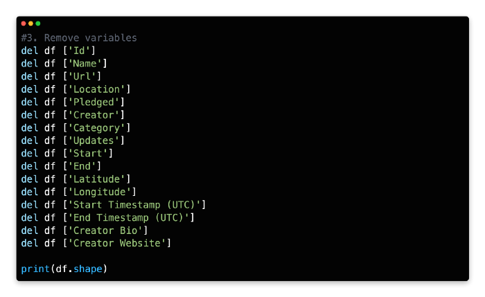
3: Remove Variables
Using the delete function, step three involves removing non-essential variables.
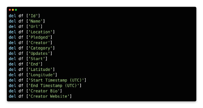
The dataframe is now empty of 16 variables. Due to the logistic regression algorithm’s inability to interpret strings or timestamps as numeric values, some variables were removed. In Step 4, you’ll be converting some of these variables using one-hot encoding, so not all non-numeric variables have been removed.

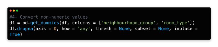
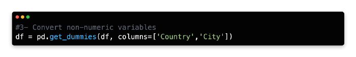
4: Convert non-numeric values
As long as discrete variables are expressed numerically, logistic regression accepts them as inputs. By using one-hot encoding, you can convert the remaining categorical features into numeric values.


5: Remove and Fill Missing Values
Next, let’s look for missing values in the data frame.


Based on the output, four of the 36 variables are missing values: these variables and their correlation with y (State_successful) are summarized in the following table.

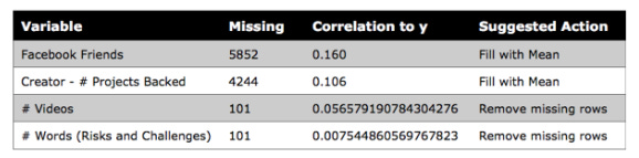
Despite many missing values, Facebook Friends and Creator — # Projects Backed variables are positively correlated with state success. The dataset would be cut in half if missing values were removed from these two variables (18,142 rows to 9,532)
Due to their low frequency (101) the missing rows can be removed. Due to their low correlation with the dependent variable, you could also remove these two variables.
The next step is to examine the standard deviation and range of the two remaining variables using the describe() method.

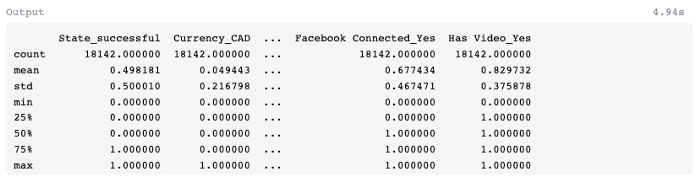
Facebook Friends has a high standard deviation (std) and range (max-min), but Creator — # Projects Backed has a lower standard deviation. As a final step, let’s use Seaborn and Matplotlib/Pyplot to plot the distribution of these variables.
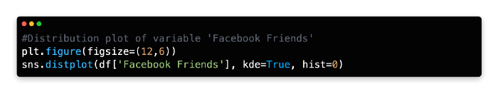

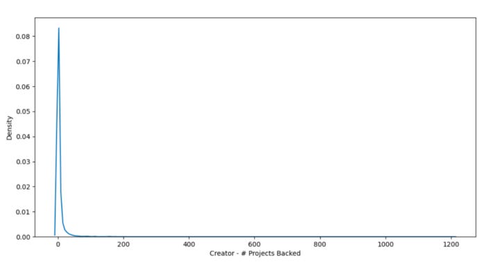
Adding a mean, mode, or other artificial value to the variable Facebook Friends is challenging due to its high variance.
In addition, there is a significant correlation between this variable and the dependent variable, so we may not necessarily want to remove it. In order to remove rows with missing values, we will retain this variable.
Similarly, Creator — # Projects Backed has a problem. This variable can, however, be filled with the mean without significantly changing the patterns in data because of its lower range, standard deviation, and correlation with the dependent variable.
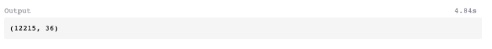
As a result of these modifications, you have 12,215 rows, which is equivalent to two-thirds of the original dataset.
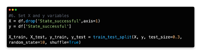
6: Set X and Y Variable
This model has the binary variable State_successful as the dependent variable (y), and the remaining variables as independent variables (X). The full data frame can be called rather than each variable being called separately as we did in the previous exercise, and the y variable can be removed using the drop method instead of calling each variable individually.
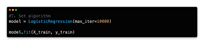
7: Set Algorithm
The LogisticRegression() method should be assigned to the variable model or a variable name of your choice.
8: Predict
Based on the input of its independent variables, let’s use our model to predict the likely outcome of a Kickstarter campaign.
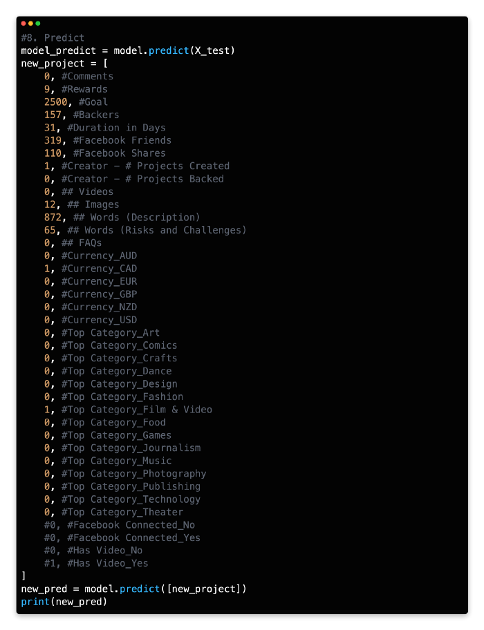
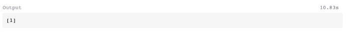
Based on the input variables and rules of our model, we predict that the new campaign will reach its target funding based on its binary outcome [1]. The campaign would be classified as unsuccessful if the binary outcome was [0].
9: Evaluate
Utilizing a confusion matrix and classification report from Scikit-learn, let’s compare the predicted results with the actual results of the Y_test set using the predict function on the X_test data.
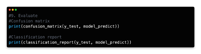
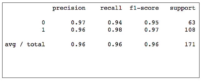
Based on the confusion matrix, 171 predictions were falsely positive and 211 were falsely negative. In spite of the high precision, recall, and f1-score conveyed in the classification report, the model’s overall performance is favorable.
Introduction To Tree-Based ML Methods
Gradient boosting, decision trees, and random forests are some of the tree-based methods covered in this lesson.
Numeric and categorical outputs are predicted with tree-based learning algorithms, also known as CART.
Boosting, bagging, random forests, decision trees, and other tree-based methods have been proven to be very effective for supervised learning. Moreover, they can predict both discrete and continuous outcomes, which explains their high accuracy.
Three tree-based algorithms will be discussed:
Decision Trees
Random Forests
Gradient Boosting
Decision Trees
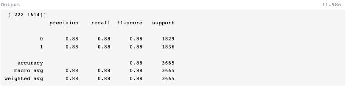
A Decision Tree (DT) creates a decision structure by dividing data into groups and interpreting patterns through those groups. Entropy (a measure of variance in data among different classes) is used to divide the data into homogeneous or numerically relevant groups. Decision trees are often graphical representations of tree-like graphs that can be easily understood by non-experts.
Random Forest
RF (Random Forests) is a technique that mitigates overfitting by growing multiple trees. For regression or classification, the results are combined by averaging the output of multiple decision trees, using a randomized selection of input data for each tree.
Gradient Boosting
A boosting technique, like random forests, aggregates the outcomes of multiple decision trees through regression and classification.
Gradient Boosting (GB) is a sequential method that improves the performance of each subsequent decision tree rather than creating random independent variants of a decision tree in parallel.
Introduction To Decision Trees
Based on entropy (the measure of variance within a class), DT creates a decision structure for interpreting patterns by classifying data into homogeneous or numerically relevant groups. Tree-like graphs are useful for displaying decision trees, and they’re easy for non-experts to understand.
It is quite different from an actual tree in that the “leaves” are located at the bottom, or foot, of the tree. Decision rules are expressed by the path from the tree’s root to its terminal leaf node. A branch represents the outcome of a decision or variable, and a leaf node represents a class label.
In order to implement DT, the following steps must be taken:
1 — Import libraries
2 — Import the dataset
3 — Convert non-numeric variables
4 — Remove columns
5 — Set X and y variables
6 — Set algorithm
7 — Evaluate
Exercise
Using the Advertising dataset, let’s use a decision tree classifier to predict a user’s click-through outcome.
Decision Trees Implementation
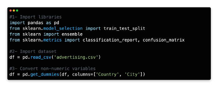
1: Import Libraries
As we will be predicting a discrete variable, we will use the classification version of the decision tree algorithm. In this example, we attempt to predict the dependent variable Clicked on Ad (0 or 1) by using the DecisionTreeClassifier algorithm from Scikit-learn. A classification report and a confusion matrix will be used to evaluate the model’s performance.

2: Import Dataset
Assign a variable name to the Advertising Dataset and import it as a data frame.

3: Convert Non-Numerical Variables
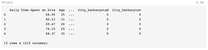
Numerical values can be obtained by encoding the Country and City variables one-at-a-time.
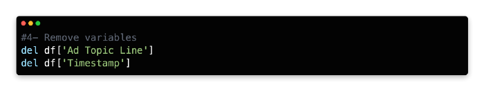
4: Remove Columns
Ad Topic Line and Timestamp are not relevant or practical for this model, so delete them.


5: Set X and Y Variables
Our dependent variable (y) is the number of times people clicked on the ad, whereas our independent variables (X) are the remaining variables. In addition to Daily Time Spent on Site, Age, Area Income, Daily Internet Usage, Male, Country, and City, there are also independent variables.

6: Set Algorithm
Assign DecisionTreeClassifier() to the variable model.

7: Evaluate
The training model should be tested on the X test data by using the predict function and a new variable name should be assigned.


Nine false negatives and ten false positives were produced by the model. Next, let’s see if we can improve predictive accuracy using multiple decision trees.
Random Forest
In addition to explaining a model’s decision structure, decision trees can also overfit the model.
A decision tree decodes patterns accurately when using training data, but since it uses a fixed sequence of paths, it can make poor predictions when using test data. In addition to having only one tree design, this method is also limited in its ability to manage variance and future outliers.
Multiple trees can be grown using a different technique called RF to mitigate overfitting. For regression or classification, multiple decision trees are grown with a randomized selection of input data for each tree and the results are combined by averaging the outputs.
A randomized and capped variable is also chosen to divide the data. Every tree in the forest would look the same if a full set of variables were examined. Each split would allow the trees to select the optimal variable according to the maximum information gain at the subsequent layer.
However, random forests algorithm does not have a full set of variables to draw from, like a standard decision tree. Because random forests use randomized data and fewer variables, they are less likely to produce similar trees. Because random forests incorporate volatility and volume, they are potentially less likely to be overfitted and provide reliable results.
In order to implement RF, the following steps must be taken:
1 — Import libraries
2 — Import dataset
3 — Convert non-numeric variables
4 — Remove columns
5 — Set X and y variables
6 — Set algorithm
7 — Evaluate
Exercise
In this exercise, we are going to repeat the previous one, but using RandomForestClassifier from Scikit-Learn to learn the dependent and independent variables.
Implementation Of Random Forest
This part will familiarize you with the implementation steps of random forest.
1: Import Libraries
In Scikit-learn, random forests can be built using either classification or regression algorithms. Scikit-learn’s RandomForestClassifier will be used here instead of RandomForestRegressor, which is used for regression.

2: Import Dataset
Import the Advertising dataset.
3: Convert non-numeric variables
Convert Country and City to numeric values using one-hot encoding.

4: Remove Variables
Data frame should be modified by removing the following two variables.
5: Set X and Y Variable
X and Y variables should be assigned the same values, and the data should be split 70/30.

6: Set Algorithm
Give RandomForestClassifier a name and specify how many estimators it should have. In general, this algorithm works best with 100–150 estimators (trees).

7: Evaluate
The predict method can be used to predict the x test values and assign them to a new variable.

A comparatively low number of false-positives (5) and false-negatives (7) were found in the test data, and the F1-score was 0.96 instead of 0.94 in the previous exercise using a decision tree classifier.
Gradient Boosting
For aggregating the results of multiple decision trees, boosting is another regression/classification technique.
It is a sequential method that aims to improve the performance of each subsequent tree, rather than creating independent variants of a decision tree in parallel. Weak models are evaluated and then weighted in subsequent rounds to mitigate misclassifications resulting from earlier rounds. A higher proportion of items are classified incorrectly at the next round than at the previous round.
This results in a weaker model, but its modifications enable it to capitalize on the mistakes of the old model. Machine learning algorithms such as gradient boosting are popular due to their ability to learn from their mistakes.
GB implementation involves the following steps:
1 — Import libraries
2 — Import dataset
3 — Convert non-numeric variables
4 — Remove variables
5 — Set X and y variables
6 — Set algorithm
7 — Evaluate
Implementation Of Gradient Booster Classifier
In this third exercise, gradient boosting will be used to predict the outcome of the Advertising dataset so that the results can be compared with those from the previous two exercises.
The regression variant of gradient boosting will be familiar to readers of Machine Learning for Absolute Beginners Second Edition. Rather than using the classification version of the algorithm in this exercise, we will use a classification version which predicts a discrete variable using slightly different hyperparameters.
1: Import Libraries
Using Scikit-learn’s ensemble package, this model uses Gradient Boosting for classification.

2: Import Dataset
The Advertising dataset should be imported and assigned as a variable.
3: Convert Non Numerical Variables
4: Remove Variables
Remove the following two variables from the data frame.
5: Set X and Y Variables
X and Y variables should be assigned the same values, and data should be split 70/30.
6: Set Algorithm
Gradient Boosting Classifier should be given a variable name and its number of estimators should be specified. With a learning rate of 0.1 and a deviance loss argument, 150–250 estimators (trees) are a good starting point for this algorithm.

7: Evaluate
Assign the predicted X test values to a new variable using the predict method.

There was one less prediction error in this model than in random forests. In spite of this, the f1-score remains 0.96, the same as random forests, but better than the classifier which was developed earlier (0.94).
Implementation of Gradient Boosting Regressor
This exercise uses gradient boosting to estimate the nightly Airbnb rate for Berlin, Germany using a regression model. Then we’ll test a sample listing based on our initial model.
1: Import Libraries
Import the following libraries:
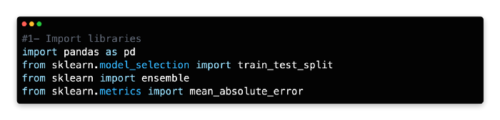
2: Import Dataset
Using the Berlin Airbnb dataset from Kaggle, we will perform this regression exercise.
The Berlin Airbnb dataset can be loaded into a Pandas dataframe by using the pd.read_csv command.
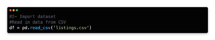
3: Remove Variable
It is not necessary to use all X variables for our model because some information overlaps between them (for example, host_name overlaps with host_id and neighborhood overlaps with neighborhood_group). Also, some variables are irrelevant, such as last_review, while others are discrete and difficult to parse, such as longitude and latitude.

4: Convert Non Numeric Variable
The neighborhood_group and room_type columns should be converted to numeric values by one-hot encoding.

5: Set X and Y Variables
The X and Y variables should be assigned. Price is the dependent variable of the Y array, while the independent variables are contained in the X array.
The data is now being divided into training and test segments. This exercise will be split 70/30 by calling Scikit-learn with a test_size of 0.3 (30%).
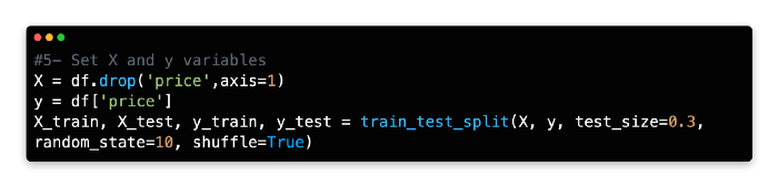
6: Set Algorithm
The following examples demonstrate how to set the initial hyperparameters for the GradientBoostingRegressor imported from Scikit-learn’s ensemble library.

7: Evaluate
To compare the difference between X_train’s expected predictions and y_train’s actual values, use the mean_absolute_error function in Scikit-learn. Up to two decimal places (%.2f) will be displayed in this example to show how accurate the model is.


We found that the mean absolute error of the training set was $22.94, and that the mean absolute error of the test set was $22.93. Therefore, the training set and test set miscalculated the actual listing price by $22.94 and $22.93, respectively. Our model shows low overfitting since both training and test data have almost identical predictions.
8: Predict
Next, let’s predict the overnight price of an individual listing using our model.

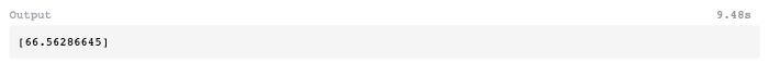
In the neighborhood of Mitte, an entire home/apartment will cost around $67.79 per night based on the model. Based on the first row of the Berlin Airbnb dataset, the actual price for this listing is $60 per night. The training and test data are shuffled randomly, and the decision trees are fed randomly with the data. If you replicate this model on your own computer, the predicted results will differ slightly.
Three tree-based algorithms will be discussed:
Decision Trees
Random Forests
Gradient Boosting
Decision Trees
A Decision Tree (DT) creates a decision structure by dividing data into groups and interpreting patterns through those groups. Entropy (a measure of variance in data among different classes) is used to divide the data into homogeneous or numerically relevant groups. Decision trees are often graphical representations of tree-like graphs that can be easily understood by non-experts.
Random Forest
RF (Random Forests) is a technique that mitigates overfitting by growing multiple trees. For regression or classification, the results are combined by averaging the output of multiple decision trees, using a randomized selection of input data for each tree.
Gradient Boosting
A boosting technique, like random forests, aggregates the outcomes of multiple decision trees through regression and classification.
Gradient Boosting (GB) is a sequential method that improves the performance of each subsequent decision tree rather than creating random independent variants of a decision tree in parallel.
Introduction To Decision Trees
Based on entropy (the measure of variance within a class), DT creates a decision structure for interpreting patterns by classifying data into homogeneous or numerically relevant groups. Tree-like graphs are useful for displaying decision trees, and they’re easy for non-experts to understand.
It is quite different from an actual tree in that the “leaves” are located at the bottom, or foot, of the tree. Decision rules are expressed by the path from the tree’s root to its terminal leaf node. A branch represents the outcome of a decision or variable, and a leaf node represents a class label.

In order to implement DT, the following steps must be taken:
1 — Import libraries
2 — Import the dataset
3 — Convert non-numeric variables
4 — Remove columns
5 — Set X and y variables
6 — Set algorithm
7 — Evaluate
Exercise
Using the Advertising dataset, let’s use a decision tree classifier to predict a user’s click-through outcome.
Decision Trees Implementation
1: Import Libraries
As we will be predicting a discrete variable, we will use the classification version of the decision tree algorithm. In this example, we attempt to predict the dependent variable Clicked on Ad (0 or 1) by using the DecisionTreeClassifier algorithm from Scikit-learn. A classification report and a confusion matrix will be used to evaluate the model’s performance.

2: Import Dataset
Assign a variable name to the Advertising Dataset and import it as a data frame.

3: Convert Non-Numerical Variables
Numerical values can be obtained by encoding the Country and City variables one-at-a-time.

4: Remove Columns
Ad Topic Line and Timestamp are not relevant or practical for this model, so delete them.


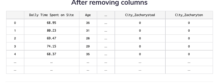
5: Set X and Y Variables
Our dependent variable (y) is the number of times people clicked on the ad, whereas our independent variables (X) are the remaining variables. In addition to Daily Time Spent on Site, Age, Area Income, Daily Internet Usage, Male, Country, and City, there are also independent variables.

6: Set Algorithm
Assign DecisionTreeClassifier() to the variable model.

7: Evaluate
The training model should be tested on the X test data by using the predict function and a new variable name should be assigned.

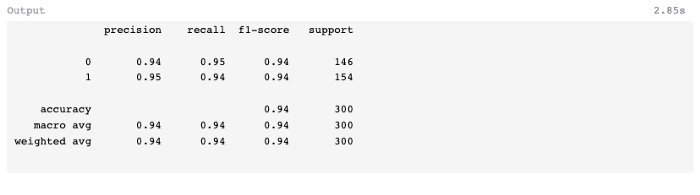
Nine false negatives and ten false positives were produced by the model. Next, let’s see if we can improve predictive accuracy using multiple decision trees.
Random Forest
In addition to explaining a model’s decision structure, decision trees can also overfit the model.
A decision tree decodes patterns accurately when using training data, but since it uses a fixed sequence of paths, it can make poor predictions when using test data. In addition to having only one tree design, this method is also limited in its ability to manage variance and future outliers.
Multiple trees can be grown using a different technique called RF to mitigate overfitting. For regression or classification, multiple decision trees are grown with a randomized selection of input data for each tree and the results are combined by averaging the outputs.
A randomized and capped variable is also chosen to divide the data. Every tree in the forest would look the same if a full set of variables were examined. Each split would allow the trees to select the optimal variable according to the maximum information gain at the subsequent layer.
However, random forests algorithm does not have a full set of variables to draw from, like a standard decision tree. Because random forests use randomized data and fewer variables, they are less likely to produce similar trees. Because random forests incorporate volatility and volume, they are potentially less likely to be overfitted and provide reliable results.
In order to implement RF, the following steps must be taken:
1 — Import libraries
2 — Import dataset
3 — Convert non-numeric variables
4 — Remove columns
5 — Set X and y variables
6 — Set algorithm
7 — Evaluate
Exercise
In this exercise, we are going to repeat the previous one, but using RandomForestClassifier from Scikit-Learn to learn the dependent and independent variables.
Implementation Of Random Forest
This part will familiarize you with the implementation steps of random forest.
1: Import Libraries
In Scikit-learn, random forests can be built using either classification or regression algorithms. Scikit-learn’s RandomForestClassifier will be used here instead of RandomForestRegressor, which is used for regression.
2: Import Dataset
Import the Advertising dataset.
3: Convert non-numeric variables
Convert Country and City to numeric values using one-hot encoding.

4: Remove Variables
Data frame should be modified by removing the following two variables.

5: Set X and Y Variable
X and Y variables should be assigned the same values, and the data should be split 70/30.
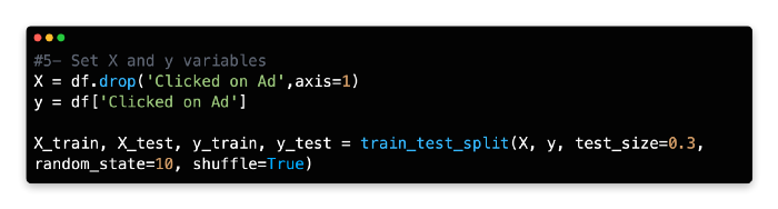
6: Set Algorithm
Give RandomForestClassifier a name and specify how many estimators it should have. In general, this algorithm works best with 100–150 estimators (trees).
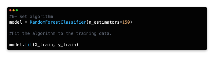
7: Evaluate
The predict method can be used to predict the x test values and assign them to a new variable.
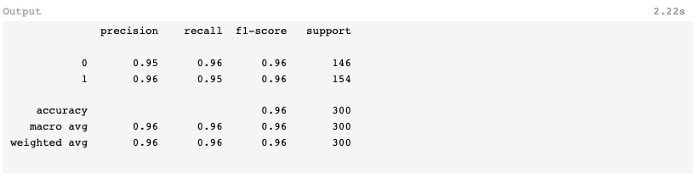
A comparatively low number of false-positives (5) and false-negatives (7) were found in the test data, and the F1-score was 0.96 instead of 0.94 in the previous exercise using a decision tree classifier.
Gradient Boosting
For aggregating the results of multiple decision trees, boosting is another regression/classification technique.
It is a sequential method that aims to improve the performance of each subsequent tree, rather than creating independent variants of a decision tree in parallel. Weak models are evaluated and then weighted in subsequent rounds to mitigate misclassifications resulting from earlier rounds. A higher proportion of items are classified incorrectly at the next round than at the previous round.
This results in a weaker model, but its modifications enable it to capitalize on the mistakes of the old model. Machine learning algorithms such as gradient boosting are popular due to their ability to learn from their mistakes.
GB implementation involves the following steps:
1 — Import libraries
2 — Import dataset
3 — Convert non-numeric variables
4 — Remove variables
5 — Set X and y variables
6 — Set algorithm
7 — Evaluate
Implementation Of Gradient Booster Classifier
In this third exercise, gradient boosting will be used to predict the outcome of the Advertising dataset so that the results can be compared with those from the previous two exercises.
The regression variant of gradient boosting will be familiar to readers of Machine Learning for Absolute Beginners Second Edition. Rather than using the classification version of the algorithm in this exercise, we will use a classification version which predicts a discrete variable using slightly different hyperparameters.
1: Import Libraries
Using Scikit-learn’s ensemble package, this model uses Gradient Boosting for classification.

2: Import Dataset
The Advertising dataset should be imported and assigned as a variable.
3: Convert Non Numerical Variables

4: Remove Variables
Remove the following two variables from the data frame.
5: Set X and Y Variables
X and Y variables should be assigned the same values, and data should be split 70/30.
6: Set Algorithm
Gradient Boosting Classifier should be given a variable name and its number of estimators should be specified. With a learning rate of 0.1 and a deviance loss argument, 150–250 estimators (trees) are a good starting point for this algorithm.
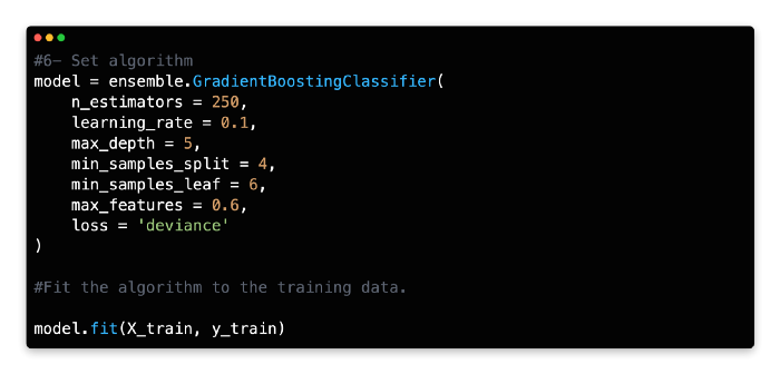
7: Evaluate
Assign the predicted X test values to a new variable using the predict method.
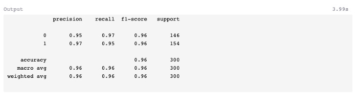
There was one less prediction error in this model than in random forests. In spite of this, the f1-score remains 0.96, the same as random forests, but better than the classifier which was developed earlier (0.94).
Implementation of Gradient Boosting Regressor
This exercise uses gradient boosting to estimate the nightly Airbnb rate for Berlin, Germany using a regression model. Then we’ll test a sample listing based on our initial model.
1: Import Libraries
Import the following libraries:

2: Import Dataset
Using the Berlin Airbnb dataset from Kaggle, we will perform this regression exercise.
The Berlin Airbnb dataset can be loaded into a Pandas dataframe by using the pd.read_csv command.

3: Remove Variable
It is not necessary to use all X variables for our model because some information overlaps between them (for example, host_name overlaps with host_id and neighborhood overlaps with neighborhood_group). Also, some variables are irrelevant, such as last_review, while others are discrete and difficult to parse, such as longitude and latitude.
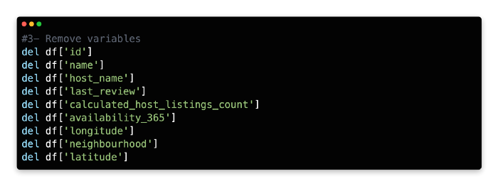
4: Convert Non Numeric Variable
The neighborhood_group and room_type columns should be converted to numeric values by one-hot encoding.

5: Set X and Y Variables
The X and Y variables should be assigned. Price is the dependent variable of the Y array, while the independent variables are contained in the X array.
The data is now being divided into training and test segments. This exercise will be split 70/30 by calling Scikit-learn with a test_size of 0.3 (30%).

6: Set Algorithm
The following examples demonstrate how to set the initial hyperparameters for the GradientBoostingRegressor imported from Scikit-learn’s ensemble library.
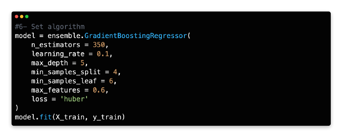
7: Evaluate
To compare the difference between X_train’s expected predictions and y_train’s actual values, use the mean_absolute_error function in Scikit-learn. Up to two decimal places (%.2f) will be displayed in this example to show how accurate the model is.

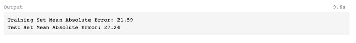
We found that the mean absolute error of the training set was $22.94, and that the mean absolute error of the test set was $22.93. Therefore, the training set and test set miscalculated the actual listing price by $22.94 and $22.93, respectively. Our model shows low overfitting since both training and test data have almost identical predictions.
8: Predict
Next, let’s predict the overnight price of an individual listing using our model.
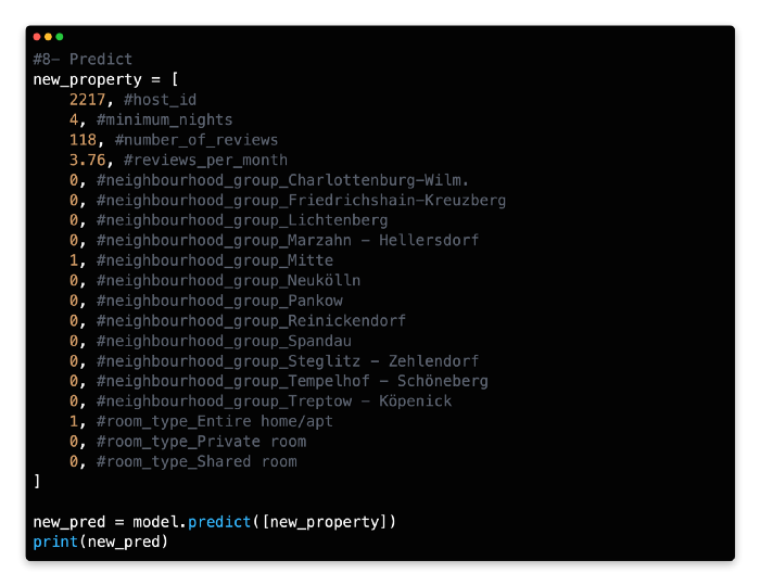

In the neighborhood of Mitte, an entire home/apartment will cost around $67.79 per night based on the model. Based on the first row of the Berlin Airbnb dataset, the actual price for this listing is $60 per night. The training and test data are shuffled randomly, and the decision trees are fed randomly with the data. If you replicate this model on your own computer, the predicted results will differ slightly.
Three tree-based algorithms will be discussed:
Decision Trees
Random Forests
Gradient Boosting
Decision Trees
A Decision Tree (DT) creates a decision structure by dividing data into groups and interpreting patterns through those groups. Entropy (a measure of variance in data among different classes) is used to divide the data into homogeneous or numerically relevant groups. Decision trees are often graphical representations of tree-like graphs that can be easily understood by non-experts.
Random Forest
RF (Random Forests) is a technique that mitigates overfitting by growing multiple trees. For regression or classification, the results are combined by averaging the output of multiple decision trees, using a randomized selection of input data for each tree.
Gradient Boosting
A boosting technique, like random forests, aggregates the outcomes of multiple decision trees through regression and classification.
Gradient Boosting (GB) is a sequential method that improves the performance of each subsequent decision tree rather than creating random independent variants of a decision tree in parallel.
Introduction To Decision Trees
Based on entropy (the measure of variance within a class), DT creates a decision structure for interpreting patterns by classifying data into homogeneous or numerically relevant groups. Tree-like graphs are useful for displaying decision trees, and they’re easy for non-experts to understand.
It is quite different from an actual tree in that the “leaves” are located at the bottom, or foot, of the tree. Decision rules are expressed by the path from the tree’s root to its terminal leaf node. A branch represents the outcome of a decision or variable, and a leaf node represents a class label.

In order to implement DT, the following steps must be taken:
1 — Import libraries
2 — Import the dataset
3 — Convert non-numeric variables
4 — Remove columns
5 — Set X and y variables
6 — Set algorithm
7 — Evaluate
Exercise
Using the Advertising dataset, let’s use a decision tree classifier to predict a user’s click-through outcome.
Decision Trees Implementation
1: Import Libraries
As we will be predicting a discrete variable, we will use the classification version of the decision tree algorithm. In this example, we attempt to predict the dependent variable Clicked on Ad (0 or 1) by using the DecisionTreeClassifier algorithm from Scikit-learn. A classification report and a confusion matrix will be used to evaluate the model’s performance.
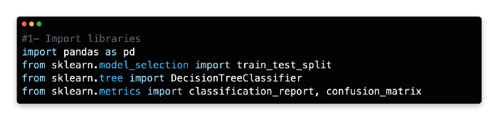
2: Import Dataset
Assign a variable name to the Advertising Dataset and import it as a data frame.
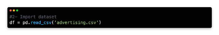
3: Convert Non-Numerical Variables
Numerical values can be obtained by encoding the Country and City variables one-at-a-time.

4: Remove Columns
Ad Topic Line and Timestamp are not relevant or practical for this model, so delete them.


5: Set X and Y Variables
Our dependent variable (y) is the number of times people clicked on the ad, whereas our independent variables (X) are the remaining variables. In addition to Daily Time Spent on Site, Age, Area Income, Daily Internet Usage, Male, Country, and City, there are also independent variables.
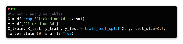
6: Set Algorithm
Assign DecisionTreeClassifier() to the variable model.
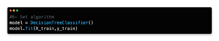
7: Evaluate
The training model should be tested on the X test data by using the predict function and a new variable name should be assigned.
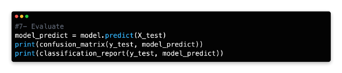

Nine false negatives and ten false positives were produced by the model. Next, let’s see if we can improve predictive accuracy using multiple decision trees.
Random Forest
In addition to explaining a model’s decision structure, decision trees can also overfit the model.
A decision tree decodes patterns accurately when using training data, but since it uses a fixed sequence of paths, it can make poor predictions when using test data. In addition to having only one tree design, this method is also limited in its ability to manage variance and future outliers.
Multiple trees can be grown using a different technique called RF to mitigate overfitting. For regression or classification, multiple decision trees are grown with a randomized selection of input data for each tree and the results are combined by averaging the outputs.
A randomized and capped variable is also chosen to divide the data. Every tree in the forest would look the same if a full set of variables were examined. Each split would allow the trees to select the optimal variable according to the maximum information gain at the subsequent layer.
However, random forests algorithm does not have a full set of variables to draw from, like a standard decision tree. Because random forests use randomized data and fewer variables, they are less likely to produce similar trees. Because random forests incorporate volatility and volume, they are potentially less likely to be overfitted and provide reliable results.
In order to implement RF, the following steps must be taken:
1 — Import libraries
2 — Import dataset
3 — Convert non-numeric variables
4 — Remove columns
5 — Set X and y variables
6 — Set algorithm
7 — Evaluate
Exercise
In this exercise, we are going to repeat the previous one, but using RandomForestClassifier from Scikit-Learn to learn the dependent and independent variables.
Implementation Of Random Forest
This part will familiarize you with the implementation steps of random forest.
1: Import Libraries
In Scikit-learn, random forests can be built using either classification or regression algorithms. Scikit-learn’s RandomForestClassifier will be used here instead of RandomForestRegressor, which is used for regression.

2: Import Dataset
Import the Advertising dataset.
3: Convert non-numeric variables
Convert Country and City to numeric values using one-hot encoding.
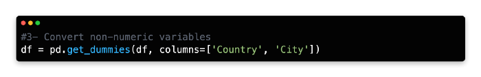
4: Remove Variables
Data frame should be modified by removing the following two variables.

5: Set X and Y Variable
X and Y variables should be assigned the same values, and the data should be split 70/30.

6: Set Algorithm
Give RandomForestClassifier a name and specify how many estimators it should have. In general, this algorithm works best with 100–150 estimators (trees).

7: Evaluate
The predict method can be used to predict the x test values and assign them to a new variable.

A comparatively low number of false-positives (5) and false-negatives (7) were found in the test data, and the F1-score was 0.96 instead of 0.94 in the previous exercise using a decision tree classifier.
Gradient Boosting
For aggregating the results of multiple decision trees, boosting is another regression/classification technique.
It is a sequential method that aims to improve the performance of each subsequent tree, rather than creating independent variants of a decision tree in parallel. Weak models are evaluated and then weighted in subsequent rounds to mitigate misclassifications resulting from earlier rounds. A higher proportion of items are classified incorrectly at the next round than at the previous round.
This results in a weaker model, but its modifications enable it to capitalize on the mistakes of the old model. Machine learning algorithms such as gradient boosting are popular due to their ability to learn from their mistakes.
GB implementation involves the following steps:
1 — Import libraries
2 — Import dataset
3 — Convert non-numeric variables
4 — Remove variables
5 — Set X and y variables
6 — Set algorithm
7 — Evaluate
Implementation Of Gradient Booster Classifier
In this third exercise, gradient boosting will be used to predict the outcome of the Advertising dataset so that the results can be compared with those from the previous two exercises.
The regression variant of gradient boosting will be familiar to readers of Machine Learning for Absolute Beginners Second Edition. Rather than using the classification version of the algorithm in this exercise, we will use a classification version which predicts a discrete variable using slightly different hyperparameters.
1: Import Libraries
Using Scikit-learn’s ensemble package, this model uses Gradient Boosting for classification.
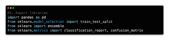
2: Import Dataset
The Advertising dataset should be imported and assigned as a variable.
3: Convert Non Numerical Variables

4: Remove Variables
Remove the following two variables from the data frame.
5: Set X and Y Variables
X and Y variables should be assigned the same values, and data should be split 70/30.
6: Set Algorithm
Gradient Boosting Classifier should be given a variable name and its number of estimators should be specified. With a learning rate of 0.1 and a deviance loss argument, 150–250 estimators (trees) are a good starting point for this algorithm.

7: Evaluate
Assign the predicted X test values to a new variable using the predict method.

There was one less prediction error in this model than in random forests. In spite of this, the f1-score remains 0.96, the same as random forests, but better than the classifier which was developed earlier (0.94).
Implementation of Gradient Boosting Regressor
This exercise uses gradient boosting to estimate the nightly Airbnb rate for Berlin, Germany using a regression model. Then we’ll test a sample listing based on our initial model.
1: Import Libraries
Import the following libraries:

2: Import Dataset
Using the Berlin Airbnb dataset from Kaggle, we will perform this regression exercise.
The Berlin Airbnb dataset can be loaded into a Pandas dataframe by using the pd.read_csv command.

3: Remove Variable
It is not necessary to use all X variables for our model because some information overlaps between them (for example, host_name overlaps with host_id and neighborhood overlaps with neighborhood_group). Also, some variables are irrelevant, such as last_review, while others are discrete and difficult to parse, such as longitude and latitude.

4: Convert Non Numeric Variable
The neighborhood_group and room_type columns should be converted to numeric values by one-hot encoding.