


Actual vs Predicted: Evaluating Stock Price Predictions
Actual vs Predicted: Evaluating Stock Price Predictions
Analyzing the Performance of a Machine Learning Model in Stock Forecasting

Predicting stock prices is a challenging yet crucial task for investors and financial analysts. In this analysis, we delve into the performance of a Long Short-Term Memory (LSTM) neural network model designed to forecast stock prices. The model is trained on historical stock data, aiming to capture the underlying patterns and trends to make accurate future predictions. We evaluate the model’s effectiveness by comparing its predictions on test data against the actual stock prices, highlighting the precision and potential areas for improvement. Through visual representation, we aim to provide a clear and concise comparison, enabling a better understanding of the model’s predictive capabilities in the dynamic and unpredictable realm of the stock market.
Please download the source code using the link provided at the conclusion of this article.
This step involves bringing in the necessary packages for use in the program.
Importing essential libraries for data analysis, visualization, and deep learning
import math # Mathematical functions
import numpy as np # Fundamental package for scientific computing with Python
import pandas as pd # Additional functions for analysing and manipulating data
import matplotlib.dates as mdates # Formatting dates
import matplotlib.pyplot as plt # Important package for visualization - we use this to plot the market data
import tensorflow as tf
from sklearn.metrics import mean_absolute_error, mean_squared_error # Packages for measuring model performance / errors
from tensorflow.keras import Sequential # Deep learning library, used for neural networks
from tensorflow.keras.optimizers import Adam
from tensorflow.keras.layers import LSTM, Dense, Dropout,Activation # Deep learning classes for recurrent and regular densely-connected layers
from tensorflow.keras.callbacks import EarlyStopping # EarlyStopping during model training
from sklearn.preprocessing import MinMaxScaler # This Scaler removes the median and scales the data according to the quantile range to normalize the price data
import seaborn as sns # Visualization
import plotly.graph_objects as go
This code imports Python libraries commonly used for mathematical and scientific calculations, data analysis, visualization, and deep learning. Each library has a specific purpose to fulfill these tasks effectively.
The math module provides functions for common mathematical operations, such as square roots and logarithms.
numpy is a key tool for scientific computing in Python. It allows users to work with extensive multi-dimensional arrays and matrices, as well as provides essential mathematical functions that can be performed on these arrays.
Pandas is a library in Python that offers added features to help with analyzing and working with data, particularly when it is structured in tables.
Matplotlib is a Python library that enables users to create various types of visualizations, such as static, animated, and interactive plots. In the context of market data, matplotlib is commonly utilized for plotting data and adjusting date formats on the plots.
Tensorflow is a library used for deep learning. It helps in creating and training neural networks.
Sklearn is a set of tools that are used for machine learning and statistical modeling. It includes various metrics that help in evaluating the performance of models.
Seaborn is a data visualization library built on top of matplotlib. It offers a simple way to generate visually appealing and informative statistical graphics.
Plotly is a tool for creating interactive visualizations like plots, charts, and graphs with various interactive features.
This code prepares the software environment for conducting data analysis, visualization, and deep learning tasks by importing the required libraries and modules.
This section involves bringing in information.
Reading and preprocessing a CSV file into a pandas DataFrame.
def read_df(csv_file):
    df = pd.read_csv(csv_file)
    df["Date"]=pd.to_datetime(df["Date"])
    df.index=df["Date"]
    df.drop("Date",axis=1,inplace=True)
    return df
csv_file = "data\\NABIL_LARGE.csv"
df = read_df(csv_file)
This code converts a CSV file into a pandas dataframe. It converts the “Date” column to a datetime format and makes it the index. Then the code removes the “Date” column and returns the updated dataframe.
You will be using the “NABIL_LARGE.csv” file, which is stored in the data folder.
DataFrame containing the data from the CSV file
df
In Python, the variable name “df” is commonly used to refer to a DataFrame object, especially within libraries like Pandas. A DataFrame is a structured way to store data in rows and columns, often used for data analysis and manipulation. The “df” variable holds this data and can be modified, analyzed, and displayed visually for further insights.
Here we will analyze and investigate the data to gain insights and understanding.
Plotting the data from the DataFrame
def plot_data(df):
    df_plot = df.copy()
    print(df_plot.shape)
    ncols = 2
    nrows = int(round(df_plot.shape[1] / ncols, 0))

    fig, ax = plt.subplots(nrows=nrows, ncols=ncols, sharex=True, figsize=(14, 7))
    for i, ax in enumerate(fig.axes):
            sns.lineplot(data = df_plot.iloc[:, i], ax=ax)
            ax.tick_params(axis="x", rotation=30, labelsize=10, length=0)
            ax.xaxis.set_major_locator(mdates.AutoDateLocator())
    fig.tight_layout()
plt.show(plot_data(df))
(4928, 6)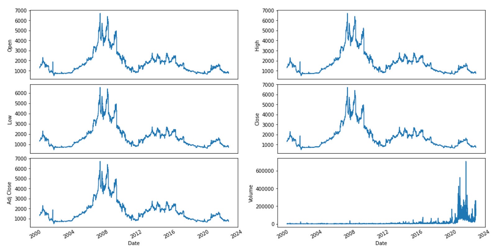
This code creates a function named ‘plot_data’ that takes a DataFrame as its input. The function makes a copy of the DataFrame and calculates the number of rows and columns needed for the plot based on the DataFrame’s shape. It then uses Matplotlib to generate a subplot figure with the defined number of rows and columns.
The function generates a line plot for each subplot using Seaborn’s ‘lineplot’ function, with the data from the respective column of the DataFrame. It further adjusts the x-axis ticks by rotating them, resizing labels, and setting the major tick locator.
The function organizes the subplots neatly by using ‘tight_layout’ and then shows the plot using Matplotlib’s ‘show’ function.
Before running this code, make sure you have imported the required libraries like pandas, matplotlib, seaborn, and matplotlib.dates.
Feature engineering is a process in machine learning where we create new input features from existing ones to help improve the performance of a model. It involves transforming, selecting, or combining features to make them more suitable for the algorithm being used. This step is crucial for building efficient and accurate machine learning models.
Creating features from the given data and returning a DataFrame
def createFeatures(data):
    data = pd.DataFrame(data)


    data['Close_Diff'] = data['Adj Close'].diff()

    data['MA200'] = data['Close'].rolling(window=200).mean()
    data['MA100'] = data['Close'].rolling(window=100).mean()
    data['MA50'] = data['Close'].rolling(window=50).mean()
    data['MA26'] = data['Close'].rolling(window=26).mean()
    data['MA20'] = data['Close'].rolling(window=20).mean()
    data['MA12'] = data['Close'].rolling(window=12).mean()

    data['DIFF-MA200-MA50'] = data['MA200'] - data['MA50']
    data['DIFF-MA200-MA100'] = data['MA200'] - data['MA100']
    data['DIFF-MA200-CLOSE'] = data['MA200'] - data['Close']
    data['DIFF-MA100-CLOSE'] = data['MA100'] - data['Close']
    data['DIFF-MA50-CLOSE'] = data['MA50'] - data['Close']

    data['MA200_low'] = data['Low'].rolling(window=200).min()
    data['MA14_low'] = data['Low'].rolling(window=14).min()
    data['MA200_high'] = data['High'].rolling(window=200).max()
    data['MA14_high'] = data['High'].rolling(window=14).max()
    data['MA20dSTD'] = data['Close'].rolling(window=20).std()

    data['EMA12'] = data['Close'].ewm(span=12, adjust=False).mean()
    data['EMA20'] = data['Close'].ewm(span=20, adjust=False).mean()
    data['EMA26'] = data['Close'].ewm(span=26, adjust=False).mean()
    data['EMA100'] = data['Close'].ewm(span=100, adjust=False).mean()
    data['EMA200'] = data['Close'].ewm(span=200, adjust=False).mean()

    data['close_shift-1'] = data.shift(-1)['Close']
    data['close_shift-2'] = data.shift(-2)['Close']

    data['Bollinger_Upper'] = data['MA20'] + (data['MA20dSTD'] * 2)
    data['Bollinger_Lower'] = data['MA20'] - (data['MA20dSTD'] * 2)

    data['K-ratio'] = 100*((data['Close'] - data['MA14_low']) / (data['MA14_high'] - data['MA14_low']) )
    data['RSI'] = data['K-ratio'].rolling(window=3).mean()

    data['MACD'] = data['EMA12'] - data['EMA26']

    nareplace = data.at[data.index.max(), 'Close']
    data.fillna((nareplace), inplace=True)

    return data
The code introduces a function named createFeatures that enhances a DataFrame by calculating and appending new columns (features) based on existing data. This code summary explains the functionality of the code. To calculate the daily closing price difference, a new column called Close_Diff is added. Moving averages, or MAs, are calculated for several time periods (200-day, 100-day, 50-day, 26-day, 20-day, and 12-day) and then added as new columns to the data. This function determines the variances between different moving averages and the closing price. It then includes these variances as additional columns in the data. This action computes the smallest and largest values for both low and high prices across various time frames, and then includes these values as new columns in the data. To determine the volatility of the closing price over a 20-day period, the standard deviation is calculated. This value is then added to the data table as a new column. The tool computes exponential moving averages (EMA) for various time periods and includes them as additional columns. Two new columns are added by shifting the closing price by 1 and 2 days, creating lagged versions of the data. The upper and lower Bollinger Bands are determined by using the 20-day moving average and standard deviation. The K-ratio and Relative Strength Index (RSI) are calculated using the lowest and highest prices observed over a 14-day period. The Moving Average Convergence Divergence (MACD) is a technical indicator that is calculated by subtracting the 26-day Exponential Moving Average (EMA) from the 12-day EMA. This action involves replacing any empty cells in the dataset with the most recent closing price available. The function ultimately returns the DataFrame with the new features included.
DataFrame with added features
df = createFeatures(df)
df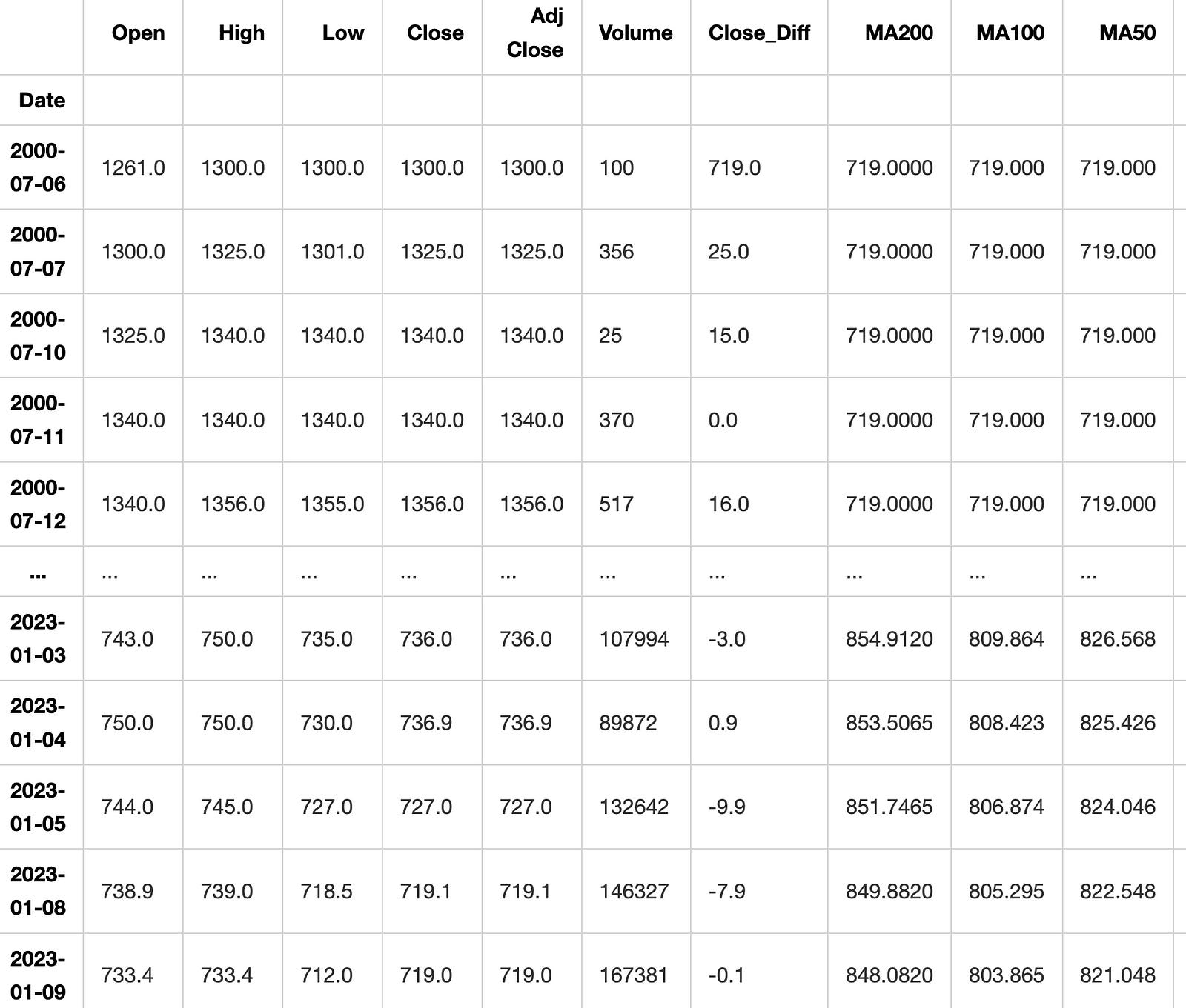
This code uses a function called “createFeatures” to modify a DataFrame named “df” by adding new columns. The function takes “df” as input and after it runs, the updated DataFrame with the new columns is printed out.
Preprocessing and feature selection are important steps in preparing data for machine learning models. Preprocessing involves cleaning, scaling, and transforming the data to make it suitable for analysis. Feature selection is the process of choosing the most relevant features in the dataset that will contribute to the predictive power of the model. These steps help improve the accuracy and efficiency of machine learning algorithms by reducing noise and redundant information in the data.
Filtering data to include only selected features
def filter_data(df):

    train_df = df.sort_values(by=['Date']).copy()

    FEATURES = ['Volume', 'High', 'Low', 'Open', 'Bollinger_Upper', 'Bollinger_Lower', 'Close'#,'RSI', 'MACD',
               ]

    print('FEATURE LIST')
    print([f for f in FEATURES])

    data = pd.DataFrame(train_df)
    data_filtered = data[FEATURES]
    return data_filtered
data_filtered = filter_data(df)
data_filtered
FEATURE LIST
['Volume', 'High', 'Low', 'Open', 'Bollinger_Upper', 'Bollinger_Lower', 'Close']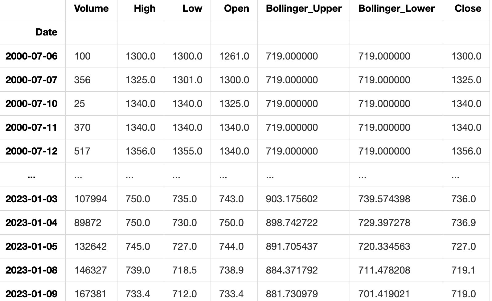
This code creates a function named filter_data which operates on a DataFrame. It begins by sorting the input DataFrame based on the ‘Date’ column, making a copy of the sorted DataFrame. It then defines a list of features called FEATURES and prints this list. Next, it converts the sorted DataFrame into a new pandas DataFrame named ‘data’. Finally, it filters the ‘data’ DataFrame to include only the columns listed in the FEATURES list and returns this filtered DataFrame.
To successfully run the code, make sure to import the pandas library at the start of your script.
Correlation of each feature with the ‘Close’ price
data_filtered.corr()['Close']Volume -0.167459
High 0.999675
Low 0.999522
Open 0.998140
Bollinger_Upper 0.972728
Bollinger_Lower 0.983736
Close 1.000000
Name: Close, dtype: float64This code computes the correlation coefficient between the ‘Close’ column and all other columns in the ‘data_filtered’ dataset. The correlation coefficient shows how the ‘Close’ column is related to each of the other columns, with a value that can range from -1 to 1. A value close to 1 indicates a strong positive relationship between the variables.
When the value is close to -1, it indicates a strong negative relationship between the variables. When a value is close to 0, it indicates that there is either no relationship or a very weak relationship between the variables being studied. This code helps determine the degree of correlation between the ‘Close’ column and the other columns in the dataset. Understanding this relationship is crucial for predictions and data analysis.
Train test split is a common technique used in machine learning to divide a dataset into two subsets: one for training the model and one for testing the model. This allows us to train the model on one portion of the data and then evaluate its performance on previously unseen data. Typically, the training subset is larger, aiding in better model training, while the testing subset helps to measure the model’s accuracy and generalization capabilities.
Splitting the dataset into train and test sets
def train_test_split(df):
    sequence_length = 100
    split_index = math.ceil(len(df) * 0.7)
    train_df = df.iloc[0:split_index, :]
    test_df = df.iloc[split_index - sequence_length:, :]
    return train_df, test_df,split_index
The code creates a function named train_test_split that uses a dataframe as its argument. The function divides the dataframe into a training set and a testing set. It does this by selecting a sequence length and splitting the data based on a 70-30 ratio, where 70% is allocated to the training set and 30% to the testing set. The variable sequence_length is assigned a value of 100, indicating that every sequence will have a length of 100. The code calculates the index to split the input dataframe by using the formula math.ceil(len(df) * 0.7). This index marks the location where 70% of the data will be used for training and the remaining 30% for testing.
It assigns the rows from the beginning up to the split index to the training dataframe called train_df. The code assigns rows in a dataframe, starting from a specific index minus a given sequence length and ending at the last row, to a new dataframe called test_df. At the end, it provides back the training data set, testing data set, and the split index. This code function divides a dataset into two sets - a training set and a testing set. The training set consists of the first 70% of the data, while the testing set contains the remaining 30% of the data plus some rows from the past based on a specified sequence length.
Test data after splitting
train_data, test_data, split = train_test_split(data_filtered)
test_data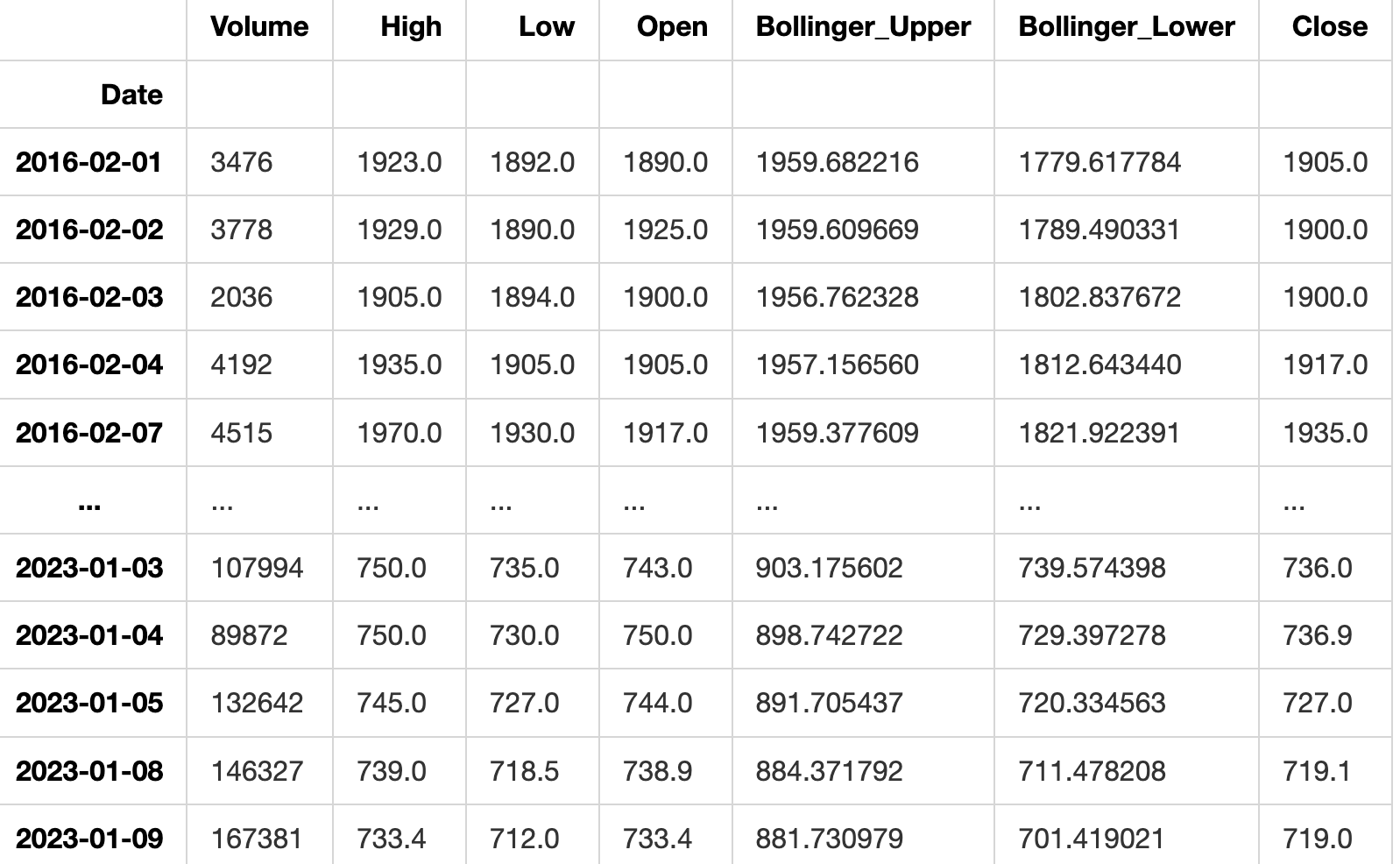
This code divides a dataset into two parts for training and testing using the train_test_split function. The training data is stored in the train_data variable, the testing data in test_data, and the ratio of the split in the split variable. Lastly, it shows the contents of the test_data variable.
Preprocessing the data by scaling it using MinMaxScaler
def preprocess_data(data):
    nrows = data.shape[0]
    np_data_unscaled = np.array(data)
    np_data = np.reshape(np_data_unscaled, (nrows, -1))
    print(np_data.shape)
    scaler = MinMaxScaler()
    np_data_scaled = scaler.fit_transform(np_data_unscaled)

    return np_data_scaled, scaler
train_data_scaled, scaler = preprocess_data(train_data)
test_data_scaled, scaler = preprocess_data(test_data)
(3450, 7)
(1578, 7)The code creates a function named preprocess_data which normalizes the input data using MinMaxScaler. This code performs the following actions: Receives input data. This step involves changing the structure or format of the input data. Displays the structure of the resized data. MinMaxScaler is utilized to rescale the data. The function returns both the scaled data and the scaling method used. The code preprocesses two sets of data, train_data and test_data, by applying a function. It then stores the scaled data and scaler in variables train_data_scaled, test_data_scaled, and scaler for future use. This command will divide the dataset into two parts: x and y.