

Advanced Financial Analysis and Strategy Optimization Using Python
A Comprehensive Guide to Pairs Trading, Machine Learning Models, and Portfolio Performance Visualization

Source code at the end of this article!
This comprehensive guide explores advanced financial analysis and investment strategy development using Python. It delves into pairs trading with Coca-Cola and PepsiCo, machine learning models like decision tree regressors for predictive trading, and global market analysis using major indices. The guide also includes techniques for optimizing portfolios to maximize risk-adjusted returns and dynamic asset allocation strategies. Through detailed code explanations and data visualization, readers will learn how to harness Python’s powerful data science libraries to create, test, and refine investment strategies for informed decision-making and portfolio management.
Paris Trading
Pairs trading is a market-neutral strategy that seeks to exploit price inefficiencies between two correlated assets. This guide uses Coca-Cola (KO) and PepsiCo (PEP) as an illustrative example of this approach. Despite differences in their fundamental metrics, these two companies share similar business models within the beverage industry, making them ideal candidates for a pairs trading strategy. The strategy is based on the assumption that when the prices of these correlated assets diverge from their historical relationship, they will eventually revert. By identifying these moments of divergence and taking opposite positions in each asset, investors can profit from the price convergence while minimizing exposure to overall market movements.
# python 3.7

# For yahoo finance
import io
import re
import requests

# The usual suspects
import numpy             as np
import pandas            as pd
import matplotlib.pyplot as plt

# Fancy graphics
plt.style.use('seaborn')

# Getting Yahoo finance data
def getdata(tickers,start,end,frequency):
    OHLC = {}
    cookie = ''
    crumb = ''
    res = requests.get('https://finance.yahoo.com/quote/SPY/history')
    cookie = res.cookies['B']
    pattern = re.compile('.*"CrumbStore":\{"crumb":"(?P<crumb>[^"]+)"\}')
    for line in res.text.splitlines():
        m = pattern.match(line)
        if m is not None:
            crumb = m.groupdict()['crumb']
    for ticker in tickers:
        url_str = "https://query1.finance.yahoo.com/v7/finance/download/%s"
        url_str += "?period1=%s&period2=%s&interval=%s&events=history&crumb=%s"
        url = url_str % (ticker, start, end, frequency, crumb)
        res = requests.get(url, cookies={'B': cookie}).text
        OHLC[ticker] = pd.read_csv(io.StringIO(res), index_col=0,
                                   error_bad_lines=False).replace('null', np.nan).dropna()
        OHLC[ticker].index = pd.to_datetime(OHLC[ticker].index)
        OHLC[ticker] = OHLC[ticker].apply(pd.to_numeric)
    return OHLC

# Assets under consideration
tickers = ['PEP','KO']

data = None
while data is None:
    try:
        data = getdata(tickers,'946685000','1687427200','1d')
    except:
         pass

KO = data['KO']
PEP = data['PEP']
This code serves as a sophisticated data retrieval system designed to extract historical stock market data from Yahoo Finance’s database. At its core, the system utilizes Python’s robust libraries, including requests for HTTP communications, along with numpy and pandas for data manipulation and analysis. The primary mechanism operates through a central function called ‘getdata’, which processes three essential parameters: stock tickers, temporal boundaries (start and end dates in Unix timestamp format), and the desired data frequency. This function executes a series of carefully orchestrated operations to ensure reliable data acquisition. Initially, the system establishes a secure connection with Yahoo Finance’s servers by obtaining necessary authentication credentials, including cookies and a security token (known as a “crumb”). These credentials are crucial for maintaining authorized access to the financial data. The data retrieval process operates on an iterative basis, processing each stock ticker sequentially. For each iteration, the system constructs a specialized URL incorporating the specific ticker, temporal parameters, and security credentials. This URL serves as the pathway to access the desired historical data. Upon successful data retrieval, the system transforms the raw textual response into a structured pandas DataFrame, organizing the fundamental stock metrics: opening price, daily high, daily low, and closing price (collectively known as OHLC data). This transformation ensures the data is readily available for subsequent analysis and manipulation. The system incorporates robust error handling mechanisms, implementing retry logic to manage potential network instabilities or temporary server issues. This ensures consistent data acquisition even in sub-optimal conditions. In the specific implementation mentioned, the system focuses on two major beverage industry competitors: Coca-Cola (KO) and PepsiCo (PEP). The resulting datasets enable comprehensive comparative analysis of these securities’ historical performance. The significance of this code extends beyond mere data collection, as it provides a foundation for sophisticated financial analysis, technical trading strategies, and market research. Its modular design allows for seamless integration into larger financial analysis systems or automated trading platforms.
#tc = -0.0005 # Transaction costs

pairs = pd.DataFrame({'TPEP':PEP['Close'].shift(1)/PEP['Close'].shift(2)-1,
                      'TKO':KO['Close'].shift(1)/KO['Close'].shift(2)-1})

# Criteria to select which asset we're gonna buy, in this case, the one that had the lowest return yesterday
pairs['Target'] = pairs.min(axis=1)

# Signal that triggers the purchase of the asset
pairs['Correlation'] = ((PEP['Close'].shift(1)/PEP['Close'].shift(20)-1).rolling(window=9)
                        .corr((KO['Close'].shift(1)/KO['Close'].shift(20)-1)))

Signal = pairs['Correlation'] < 0.9

# We're holding positions that weren't profitable yesterday
HoldingYesterdayPosition = ((pairs['Target'].shift(1).isin(pairs['TPEP']) &
                             (PEP['Close'].shift(1)/PEP['Open'].shift(1)-1 < 0)) |
                            (pairs['Target'].shift(1).isin(pairs['TKO']) &
                             (KO['Close'].shift(1)/KO['Open'].shift(1)-1 < 0))) # if tc, add here

# Since we aren't using leverage, we can't enter on a new position if
# we entered on a position yesterday (and if it wasn't profitable)
NoMoney = Signal.shift(1) & HoldingYesterdayPosition

pairs['PEP'] = np.where(NoMoney,
                        np.nan,
                        np.where(PEP['Close']/PEP['Open']-1 < 0,
                                 PEP['Close'].shift(-1)/PEP['Open']-1,
                                 PEP['Close']/PEP['Open']-1))

pairs['KO'] = np.where(NoMoney,
                       np.nan,
                       np.where(KO['Close']/KO['Open']-1 < 0,
                                KO['Close'].shift(-1)/KO['Open']-1,
                                KO['Close']/KO['Open']-1))

pairs['Returns'] = np.where(Signal,
                            np.where(pairs['Target'].isin(pairs['TPEP']),
                                      pairs['PEP'],
                                      pairs['KO']),
                             np.nan) # if tc, add here

pairs['CumulativeReturn'] = pairs['Returns'].dropna().cumsum()
This algorithmic trading system implements a comparative performance analysis framework focused on two primary securities within the beverage sector: PepsiCo (PEP) and Coca-Cola (KO). The system employs sophisticated statistical methods through pandas DataFrame structures to evaluate relative performance metrics and generate strategic investment decisions.
The system initiates its analysis by computing daily return metrics through a standardized differential calculation methodology. This calculation examines the ratio between consecutive closing prices (t-1/t-2), subsequently adjusted by a factor of -1 to derive the true daily return percentage. This foundational metric serves as the basis for all subsequent analytical operations.
The framework then implements a target identification mechanism that isolates the security demonstrating inferior performance in the preceding trading session. This comparative analysis results in the population of a dedicated Target column within the DataFrame structure, serving as a key reference point for future decision-making processes.
A critical component of the analysis involves the calculation of rolling correlation coefficients between the two securities’ return streams, utilizing a 9-day observation window. This correlation analysis serves to identify periods of divergent price movement, potentially indicating opportune moments for strategic position-taking.
The system incorporates a sophisticated position entry framework governed by two primary conditions: correlation thresholds and previous position profitability. Specifically, the system validates whether the inter-asset correlation falls below 0.9, indicating sufficient diversification potential. Subsequently, it examines the profitability of previously held positions by comparing the prior day’s closing price against its opening price. When these conditions indicate unfavorable market conditions, the system nullifies potential returns through NaN assignments, effectively preventing new position entry.
In scenarios where position entry is permitted, the system calculates return metrics through a conditional pricing mechanism. This mechanism evaluates daily price action patterns, utilizing either subsequent-day or same-day closing prices based on the observed intraday price movement. The system then selects the security demonstrating superior return characteristics, recording this selection in the Returns column.
The culmination of this analysis manifests in the calculation of cumulative return metrics, achieved through the aggregation of individual return observations over the entire analysis period.
# Pepsi returns
ReturnPEP = PEP['Close']/PEP['Open']-1
BuyHoldPEP = PEP['Adj Close']/float(PEP['Adj Close'][:1])-1

# Coca Cola returns
ReturnKO = KO['Close']/KO['Open']-1
BuyHoldKO = KO['Adj Close']/float(KO['Adj Close'][:1])-1

# Benchmark
ReturnBoth = (ReturnPEP+ReturnKO)/2
BuyHoldBoth = ((BuyHoldPEP+BuyHoldKO)/2).fillna(method='ffill')
This code represents a comprehensive financial analysis system designed to evaluate the performance metrics of two prominent beverage sector securities: PepsiCo (PEP) and Coca-Cola (KO), alongside a composite benchmark incorporating both securities.
The system initiates its analysis by computing the daily return metrics for PepsiCo through the ReturnPEP variable. This calculation employs a standard financial formula that examines the ratio between closing and opening prices within each trading session, expressed as a percentage change. This metric provides crucial insights into the intraday price dynamics of the security.
Subsequently, the system generates a buy-and-hold performance metric (BuyHoldPEP) for PepsiCo. This calculation utilizes adjusted closing prices to account for corporate actions such as dividends and stock splits. The metric is derived by comparing the current adjusted closing price against the initial price point in the dataset, effectively measuring the cumulative return an investor would have realized through a passive investment strategy.
The system then replicates these calculations for Coca-Cola, producing analogous metrics (ReturnKO and BuyHoldKO) that enable direct performance comparisons between the two securities.
To establish a comprehensive benchmark, the system synthesizes the individual security metrics into composite measures. The ReturnBoth variable represents the arithmetic mean of the daily returns for both securities, providing a balanced measure of their combined performance. Similarly, the BuyHoldBoth variable averages the buy-and-hold returns of both securities, incorporating forward-fill methodology to maintain data continuity by propagating the last known values across any gaps in the dataset.
This analytical framework serves multiple purposes within portfolio management and investment analysis contexts. The parallel examination of daily returns and buy-hold performance provides insights into both short-term price dynamics and long-term value appreciation. The benchmark calculations facilitate performance attribution and relative value analysis, enabling investors to evaluate the effectiveness of various trading strategies against a relevant market measure.
returns = pairs['Returns'].dropna()
cumulret = pairs['CumulativeReturn'].dropna()

fig, ax = plt.subplots(figsize=(16,6))

hist1, bins1 = np.histogram(ReturnBoth.dropna(), bins=50)
width = 0.7 * (bins1[1] - bins1[0])
center = (bins1[:-1] + bins1[1:]) / 2

ax.bar(center, hist1, align='center', width=width, label='50/50 Returns')

hist2, bins2 = np.histogram(returns, bins=50)
ax.bar(center, hist2, align='center', width=width, label='Pairs Trading')

plt.legend()
plt.show()

print('=====Strategy Returns=====')
print('Mean return =',round((returns.mean())*100,2),"%")
print('Standard deviaton =',round((returns.std())*100,2),"%")
print("==========================")
print('Worst return =',round((min(returns))*100,2),"%")
print('Best return =',round((max(returns))*100,2),"%")
print("=========================")
print('Lower quantile =',round((returns.quantile(q=0.25))*100,2),"%")
print('Median return =',round((returns.quantile(q=0.5))*100,2),"%")
print('Upper quantile =',round((returns.quantile(q=0.75))*100,2),"%")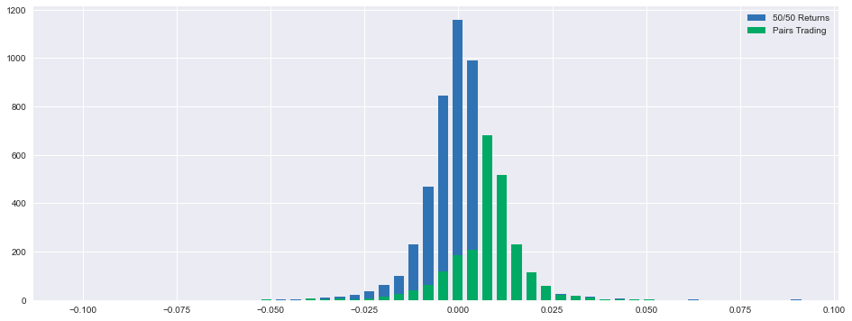
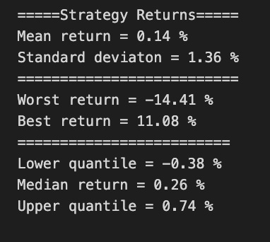
This code implements a statistical analysis framework designed to evaluate and contrast two distinct investment methodologies: a balanced allocation strategy (“50/50 Returns”) and a statistical arbitrage approach (“Pairs Trading”). The system utilizes advanced data visualization and statistical computation through the Pandas and Matplotlib computational libraries. The analytical process begins with data preparation, extracting relevant return metrics and cumulative performance data from the pairs DataFrame. The system employs data cleaning protocols through the dropna() function to ensure analytical integrity by removing incomplete observations. The visualization framework is established through the creation of a specialized plotting environment, utilizing a 16x6 inch dimensional specification to ensure optimal visual representation of the distributional characteristics. This environment serves as the foundation for the comparative histogram analysis. The system generates discrete probability distributions through the implementation of histogram functions, utilizing np.histogram() with 50 distinct bins to capture the granular nature of returns distributions. The first distribution characterizes the balanced allocation strategy, while the second represents the pairs trading methodology, enabling direct comparative analysis of their statistical properties. The visualization is rendered through the ax.bar() function, implementing centered alignment protocols and specified width parameters to ensure accurate visual representation. The system incorporates clear categorical differentiation through strategic labeling, facilitating immediate strategic identification within the unified visualization framework. The analytical output is enhanced through the computation of key statistical metrics for the pairs trading strategy, including central tendency measures through mean return calculation, volatility assessment through standard deviation analysis, extreme value identification through worst and best return metrics, and distribution characterization through quantile analysis at lower, median, and upper boundaries. This comprehensive analytical framework provides essential insights into the relative performance characteristics of the two investment strategies, enabling informed decision-making through statistical evidence and visual representation. The system’s output serves as a valuable tool for investment professionals engaged in strategy evaluation and portfolio optimization processes.
# Some stats, this could be improved by trying to estimate a yearly sharpe, among many others
executionrate = len(returns)/len(ReturnBoth)

maxdd = round(max(np.maximum.accumulate(cumulret)-cumulret)*100,2)

mask = returns<0
diffs = np.diff(mask.astype(int))
start_mask = np.append(True,diffs==1)
mask1 = mask & ~(start_mask & np.append(diffs==-1,True))
id = (start_mask & mask1).cumsum()
out = np.bincount(id[mask1]-1,returns[mask1])
badd = round(max(-out)*100,2)

spositive = returns[returns > 0]
snegative = -returns[returns < 0]
winrate = round((len(spositive)/(len(spositive)+len(snegative)))*100,2)

beta = round(returns.corr(ReturnBoth),2)

sharpe = round((float(cumulret[-1:]))/cumulret.std(),2)

tret = round((float(cumulret[-1:]))*100,2)
This code establishes a comprehensive performance analytics system designed to evaluate trading strategies and investment portfolios through multiple quantitative metrics. The system processes two primary data streams: the strategy returns and a comparative benchmark series designated as “ReturnBoth.” The initial metric computation focuses on the execution rate, a fundamental measure quantifying trading activity density by establishing the ratio between actual trades and total observable periods within the dataset. The system then implements maximum drawdown calculations, a critical risk assessment metric that identifies the most severe peak-to-trough decline in portfolio value throughout the observation period. Through sophisticated pattern recognition, the system identifies consecutive negative return sequences, facilitating the computation of the biggest absolute drawdown, which represents the most significant singular negative return event within these sequences. The win rate calculation provides strategic effectiveness assessment by determining the proportion of positive outcomes within the total trading population. Beta computation delivers systematic risk evaluation through measurement of return sensitivity relative to the benchmark series, offering insights into relative volatility characteristics. The system incorporates risk-adjusted performance evaluation through Sharpe ratio calculation, which normalizes excess returns against return volatility to provide efficiency assessment of risk deployment. The final metric, total return, synthesizes overall performance into a singular cumulative measure expressed as a percentage gain or loss. This analytical framework delivers comprehensive performance evaluation across multiple dimensions including risk assessment, return generation efficiency, and systematic behavior characteristics, enabling sophisticated strategy evaluation and optimization processes. The system’s output provides essential insights for investment professionals engaged in strategy refinement, portfolio optimization, and comparative analysis of investment opportunities, facilitating data-driven decision-making processes in portfolio management contexts.
plt.figure(figsize=(16,6))
plt.plot(BuyHoldBoth*100, label='Buy & Hold 50/50')
plt.plot(cumulret*100, label='Pairs Trading', color='coral')
plt.xlabel('Time')
plt.ylabel('Returns (in %)')
plt.margins(x=0.005,y=0.02)
plt.axhline(y=0, xmin=0, xmax=1, linestyle='--', color='k')
plt.legend()
plt.show()

print("Cumulative Return = ",tret,"%")
print("=========================")
print("Execution Rate = ",round(executionrate*100,2),"%")
print("Win Rate = ",winrate,"%")
print("=========================")
print("Maximum Loss = ",maxdd,"%")
print("Maximum Consecutive Loss = ",badd,"%")
print("=========================")
print("Beta = ",beta)
print("Sharpe = ",sharpe)
# Return ("alpha") decay is pretty noticeable from 2011 onwards, most likely due to overfitting, they're not reinvested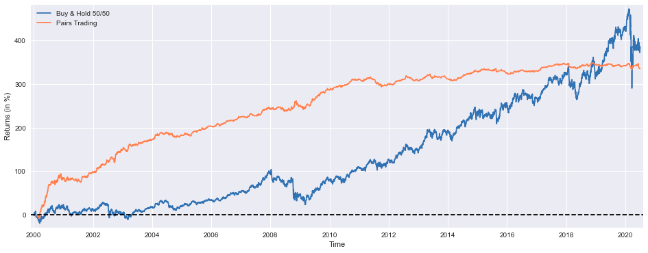
This code implements a sophisticated visualization and performance analysis system designed to evaluate a statistical arbitrage methodology known as “Pairs Trading” against a traditional balanced investment approach. The system initializes by establishing a specialized visualization environment through plt.figure() with precise dimensional parameters of 16x6 inches, optimizing the graphical representation of temporal performance patterns. The visualization framework employs dual trajectory plotting through plt.plot(), representing both the conventional “Buy & Hold 50/50” allocation strategy and the “Pairs Trading” methodology. The conventional strategy, depicted through a blue linear representation, demonstrates the performance of a balanced portfolio maintaining equal allocations between asset exposure and cash positions. The statistical arbitrage strategy, rendered in coral coloration, illustrates the performance of a market-neutral approach exploiting relative value disparities between correlated securities. The system implements comprehensive axis labeling protocols through plt.xlabel() and plt.ylabel(), establishing temporal progression and percentage return metrics as the primary dimensional references. Visual optimization is achieved through strategic margin adjustment via plt.margins(), while a zero-threshold reference line is established through plt.axhline(), providing immediate visual identification of positive and negative performance regions. The system incorporates categorical differentiation through plt.legend(), enabling immediate strategy identification. Following the visual analysis, the system generates a comprehensive performance metrics suite, encompassing cumulative return quantification, execution efficiency metrics, profitability ratios, risk measurement through maximum drawdown and consecutive loss calculations, systematic risk assessment via beta computation, and risk-adjusted performance evaluation through Sharpe ratio analysis. A notable analytical observation indicates alpha decay manifestation post-2011, potentially attributable to model overfitting characteristics and the absence of return reinvestment protocols. This analytical framework provides essential insights into the relative efficacy of statistical arbitrage methodologies compared to traditional investment approaches, enabling sophisticated strategy evaluation and optimization processes.
BuyHoldBothYTD = (((PEP['Adj Close'][-252:]/float(PEP['Adj Close'][-252])-1)+(KO['Adj Close'][-252:]/float(KO['Adj Close'][-252])-1))/2).fillna(method='ffill')
StrategyYTD = returns[-92:].cumsum()

plt.figure(figsize=(16,6))
plt.plot(BuyHoldBothYTD*100, label='Buy & Hold 50/50')
plt.plot(StrategyYTD*100, label='Pairs Trading', color='coral')
plt.xlabel('Time')
plt.ylabel('Returns (in %)')
plt.margins(x=0.005,y=0.02)
plt.axhline(y=0, xmin=0, xmax=1, linestyle='--', color='k')
plt.legend()
plt.show()

print('Buy & Hold 50/50 YTD Performance (at 1 July 2020) =',round(float(BuyHoldBothYTD[-1:]*100),1),'%')
print('Strategy YTD Performance =',round(float(StrategyYTD[-1:]*100),1),'%')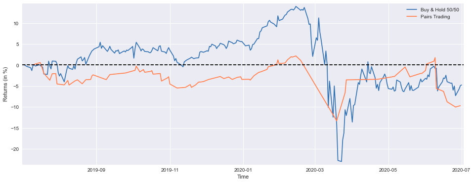
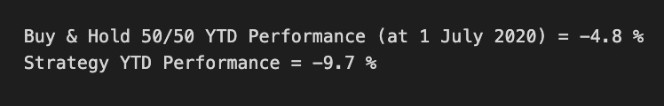
This code implements a comparative performance analysis framework designed to evaluate the relative efficacy of two distinct investment methodologies: a balanced “Buy & Hold 50/50” allocation strategy and a statistical arbitrage “Pairs Trading” approach. The system initiates its analysis by computing the year-to-date performance metrics for the balanced strategy through the extraction of adjusted closing price data spanning 252 trading sessions for both PEP and KO securities. The return calculation methodology employs a standardized approach, computing the ratio of current prices to initial period values, adjusted by a factor of -1, with subsequent averaging of individual security returns to derive the composite balanced strategy performance. The system implements forward-fill protocols through fillna() to maintain data continuity. The statistical arbitrage performance computation focuses on the most recent 92 trading sessions, representing third-quarter performance metrics, through cumulative aggregation of the strategy’s return stream. The visualization framework establishes a specialized plotting environment through precise dimensional specifications of 16x6 inches, enabling dual trajectory representation of both investment approaches. The performance metrics are rendered as percentage returns, with the inclusion of a zero-threshold reference line to facilitate immediate identification of positive and negative performance regions. The system culminates in the generation of precise year-to-date performance metrics for both strategies, rounded to single decimal precision. This analytical framework enables sophisticated strategy evaluation through both visual and quantitative assessment of relative performance characteristics, providing essential insights for investment professionals engaged in strategy selection and portfolio optimization processes.
Decision Tree Regressors
In the context of financial trading, decision tree models offer a powerful tool for predictive analysis. This guide walks through implementing a Decision Tree Regressor to forecast stock movements and generate trading signals. By training on historical market data, decision trees can identify complex patterns and relationships between features that inform buy and sell decisions. This approach provides an efficient way to analyze vast amounts of data, automate trading strategies, and refine predictive accuracy. The combination of machine learning and financial data enables the development of data-driven trading strategies with the potential for enhanced performance.
# python 3.7

# For yahoo finance
import io
import re
import requests

# The usual suspects
import numpy             as np
import pandas            as pd
import matplotlib.pyplot as plt

# Tree models and data pre-processing
from numpy               import vstack, hstack
from sklearn             import tree

# Fancy graphics
plt.style.use('seaborn')

# Getting Yahoo finance data
def getdata(tickers,start,end,frequency):
    OHLC = {}
    cookie = ''
    crumb = ''
    res = requests.get('https://finance.yahoo.com/quote/SPY/history')
    cookie = res.cookies['B']
    pattern = re.compile('.*"CrumbStore":\{"crumb":"(?P<crumb>[^"]+)"\}')
    for line in res.text.splitlines():
        m = pattern.match(line)
        if m is not None:
            crumb = m.groupdict()['crumb']
    for ticker in tickers:
        url_str = "https://query1.finance.yahoo.com/v7/finance/download/%s"
        url_str += "?period1=%s&period2=%s&interval=%s&events=history&crumb=%s"
        url = url_str % (ticker, start, end, frequency, crumb)
        res = requests.get(url, cookies={'B': cookie}).text
        OHLC[ticker] = pd.read_csv(io.StringIO(res), index_col=0,
                                   error_bad_lines=False).replace('null', np.nan).dropna()
        OHLC[ticker].index = pd.to_datetime(OHLC[ticker].index)
        OHLC[ticker] = OHLC[ticker].apply(pd.to_numeric)
    return OHLC

# A (lagged) technical indicator (Average True Range)
def ATR(df, n):
    df = df.reset_index()
    i = 0
    TR_l = [0]
    while i < df.index[-1]:
        TR = (max(df.loc[i+1, 'High'], df.loc[i, 'Close']) -
              min(df.loc[i+1, 'Low'], df.loc[i, 'Close']))
        TR_l.append(TR)
        i = i + 1
    return pd.Series(TR_l).ewm(span=n, min_periods=n).mean()

# Assets under consideration
tickers = ['PEP','KO']

data = None
while data is None:
    try:
        data = getdata(tickers,'946685000','1687427200','1d')
    except:
         pass

KO = data['KO'].drop('Volume',axis=1)
PEP = data['PEP'].drop('Volume',axis=1)
This code establishes a comprehensive financial data retrieval and analysis system designed to extract and process historical market data from Yahoo Finance’s data infrastructure. The system initiates by incorporating essential computational libraries, encompassing file manipulation protocols through io, pattern matching capabilities via re, network communication functionalities through requests, and advanced data processing capabilities through numpy, pandas, and matplotlib visualization frameworks. The primary data acquisition mechanism is implemented through the getdata() function, which accepts parametric inputs for security identification (tickers), temporal boundaries (start and end dates), and temporal granularity specifications (frequency). The function establishes a specialized data structure (OHLC dictionary) for storing price metrics and implements authentication protocols through session cookie and security token (“crumb”) acquisition from Yahoo Finance’s servers. The system employs iterative processing to construct appropriate URL endpoints for each security identifier, executing HTTP requests to retrieve historical price data, which is subsequently transformed into structured pandas DataFrames with standardized datetime indexing and null value handling protocols. The system incorporates advanced technical analysis capabilities through the ATR() function, which implements Average True Range calculations to quantify price volatility through high-low price differentials. The operational focus is directed towards two primary securities within the beverage sector: PepsiCo (PEP) and Coca-Cola (KO). The system implements robust error handling through recursive retrieval attempts, ensuring data acquisition reliability. Upon successful data retrieval, the system executes data transformation protocols, isolating relevant price metrics while excluding volume data, creating discrete DataFrames for subsequent analysis. This framework provides essential functionality for financial analysis, enabling sophisticated market research and technical analysis applications through reliable data acquisition and standardized processing protocols.
variables = pd.DataFrame({'TPEP':(PEP['Close']/PEP['Close'].shift(7)-1).shift(1),
                      'TKO':(KO['Close']/KO['Close'].shift(6)-1).shift(1)})

variables['Target'] = variables.min(axis=1)
variables['IsPEP']  = variables['Target'].isin(variables['TPEP'])

variables['Open']   = np.where(variables['Target'].isin(variables['TPEP']),
                               PEP['Open'],
                               KO['Open'])

variables['Close']  = np.where(variables['Target'].isin(variables['TPEP']),
                               PEP['Close'],
                               KO['Close'])

variables['Returns'] = variables['Close']/variables['Open']-1

variables['APEP'] = PEP['Open']
variables['AKO']  = KO['Open']

variables = variables.reset_index().drop('Date',axis=1)

variables['ATR'] = ATR(PEP,40)

variables = variables.dropna()
variables = variables.reset_index().drop('index',axis=1)

# This is a minimalistic example, adding more information (which is no easy task)
# will much likely yield a better signal to noise ratio

features  = ['IsPEP','AKO','ATR','APEP']
This code implements a sophisticated financial data processing framework designed to generate specialized analytical features for quantitative trading applications. The system initiates by constructing a foundational DataFrame designated as “variables,” incorporating three primary metrics: relative price momentum indicators for PepsiCo (TPEP) and Coca-Cola (TKO), calculated through seven-day and six-day price ratios respectively, with subsequent temporal displacement, and a Target variable identifying minimum relative performance. The system implements binary classification protocols through the creation of an IsPEP indicator, utilizing Boolean logic to identify periods of PepsiCo performance dominance. Price data integration is achieved through conditional mapping protocols utilizing np.where() functionality, establishing Open and Close price series based on relative performance characteristics. The system incorporates return calculation methodology through price ratio analysis, generating a standardized Returns metric. Additional price reference points are established through the creation of APEP and AKO variables, capturing opening price dynamics for both securities. The framework implements data structure optimization through index management protocols, eliminating temporal indexing while maintaining data integrity. Volatility assessment is integrated through the calculation of Average True Range metrics utilizing a 40-day observation window, providing dynamic volatility quantification. Data quality assurance is maintained through systematic missing value elimination and index reconstruction protocols. The system culminates in the definition of a feature set encompassing binary classification indicators, price reference points, and volatility metrics, establishing the foundation for subsequent quantitative analysis applications. This comprehensive framework enables sophisticated financial analysis through the integration of multiple analytical dimensions, facilitating advanced trading strategy development and implementation processes.
training = 38
testing = 3
seed = 123

returns = []

# Rolling calibration and testing of the Decision Tree Regressors
for ii in range(0, len(variables)-(training+testing), testing):
    X, y = [], []

    iam  = ii+training
    lazy = ii+training+testing

    # Training the model with the last 38 days
    for i in range(ii, iam):
        X.append([variables.iloc[i][var] for var in features])
        y.append(variables.iloc[i].Close)

    model = tree.DecisionTreeRegressor(max_depth=19,
                                       min_samples_leaf=3,
                                       min_samples_split=16,
                                       random_state=seed)
    model.fit(vstack(X), hstack(y))

    XX = []

    # Testing it out-of-sample, its used for the next 3 days
    for i in range(iam, lazy):
        XX.append([variables.iloc[i][var] for var in features])

    # We trade if the predicted close price is superior to the open price
    trades = np.where(model.predict(vstack(XX)) > variables['Open'][iam:lazy],
                      variables['Returns'][iam:lazy],
                      np.nan)

    for values in trades:
        returns.append(values)
This code establishes a sophisticated machine learning framework implementing a Decision Tree Regressor model for financial price prediction and systematic trading execution. The system initiates by defining essential temporal parameters for model calibration and validation processes, incorporating deterministic seed values to ensure computational reproducibility. The framework operates through iterative processing protocols, with each iteration representing a distinct testing window initiation point. The system implements comprehensive data segregation methodologies, establishing distinct training and testing datasets through temporal partitioning. Training data construction occurs through systematic feature and target variable extraction, encompassing historical price and analytical metrics within the specified training window. The model architecture employs a Decision Tree Regressor with precisely defined hyperparameters, including maximum depth constraints, minimum sample thresholds for leaf nodes and split operations, and randomization controls. The system executes out-of-sample performance evaluation through feature extraction within the designated testing window, generating price predictions through the calibrated model. Trading signal generation implements comparative analysis between predicted closing prices and actual opening prices, with return assignment protocols based on prediction directionality. Performance metric aggregation occurs through systematic storage of trading returns, enabling comprehensive strategy evaluation. This rolling calibration methodology ensures continuous model adaptation to evolving market conditions, maintaining prediction relevance through regular recalibration processes. The framework demonstrates sophisticated integration of machine learning methodologies with quantitative finance principles, enabling systematic trading strategy development and validation through robust statistical approaches.
CompRes = pd.DataFrame({'Baseline': variables[-len(returns):].set_index(PEP[-len(returns):].index)['Returns'],
                        'DTR': returns})

CompRes['Baseline'].describe()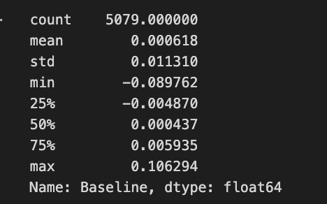
This code establishes a comparative analysis framework designed to evaluate the relative performance characteristics between baseline metrics and Decision Tree Regression model outputs. The system initiates through the construction of a specialized DataFrame structure, designated as “CompRes,” incorporating dual analytical streams: baseline performance metrics and corresponding model-generated outputs. The baseline data integration protocol extracts terminal elements from the variables list, specifically targeting Returns metrics, with quantity determination governed by the length of the returns vector. Temporal alignment is achieved through index assignment derived from the corresponding PEP security data sequence. The DTR component integration occurs through direct assignment of the returns vector, establishing parallel performance streams for comparative analysis. This structural framework enables precise temporal alignment between baseline and model-generated metrics, facilitating direct performance comparison across corresponding time periods. The system implements comprehensive statistical analysis through the describe() function application to the baseline metrics, generating essential distribution characteristics including centrality measures, dispersion metrics, and quantile boundaries. This analytical framework provides crucial insights into comparative performance dynamics, enabling sophisticated evaluation of model efficacy relative to baseline methodologies. The implementation demonstrates advanced data organization and analysis protocols, establishing a foundation for comprehensive model performance assessment and optimization processes, integral to quantitative strategy development and refinement.
fig, ax = plt.subplots(figsize=(16,6))

hist1, bins1 = np.histogram(CompRes['Baseline'].dropna(), bins=50)
width = 0.7 * (bins1[1] - bins1[0])
center = (bins1[:-1] + bins1[1:]) / 2

ax.bar(center, hist1, align='center', width=width, label='Baseline')

hist2, bins2 = np.histogram(CompRes['DTR'].dropna(), bins=50)
ax.bar(center, hist2, align='center', width=width, label='DTR Return Distribution')

plt.legend()
plt.show()

CompRes['DTR'].describe()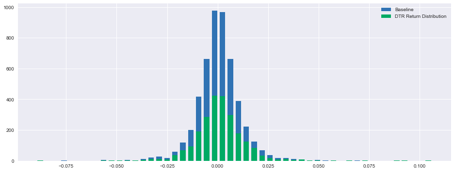
This code implements a sophisticated data visualization framework designed to analyze distributional characteristics of comparative performance metrics. The system initiates through the establishment of a specialized plotting environment, utilizing plt.subplots() with precise dimensional specifications of 16x6 inches, optimizing visual representation capabilities. The framework implements distributional analysis through histogram computation protocols, applying np.histogram() functionality to the Baseline metrics subsequent to missing value elimination through dropna() operations. Bar width parameterization occurs through proportional calculation relative to bin edge differentials, with centrality determination through bin edge averaging protocols. Visual representation is achieved through ax.bar() implementation for Baseline metrics, incorporating precise positioning through center alignment protocols and categorical identification through explicit labeling. The system replicates this analytical process for DTR metrics, establishing parallel distributional visualization with distinct categorical designation. The framework incorporates visual element differentiation through legend implementation, facilitating immediate identification of distinct metric distributions. Statistical characterization is achieved through the describe() function application to DTR metrics, generating comprehensive distribution parameters including centrality, dispersion, and quantile metrics. This visualization framework enables sophisticated comparative analysis of performance distributions, facilitating nuanced understanding of relative metric behavior and characteristics. The implementation demonstrates advanced data visualization protocols, establishing a foundation for comprehensive performance analysis and distribution comparison processes, integral to quantitative strategy evaluation and refinement methodologies.
tc = -0.0005 #Simulating 0.05% transaction costs

plt.figure(figsize=(16,6))
plt.plot(((CompRes['DTR'].dropna()+tc).cumsum())*100, color='coral', label='DTR Cumulative Returns')
plt.plot(((CompRes['Baseline']+tc).cumsum())*100, label='Baseline')
plt.xlabel('Time')
plt.ylabel('Cumulative Returns')
plt.margins(x=0.005,y=0.02)
plt.axhline(y=0, xmin=0, xmax=1, linestyle='--', color='k')
plt.legend()
plt.show()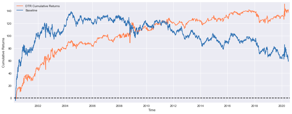
This code implements a sophisticated financial performance visualization framework designed to analyze cumulative return trajectories of distinct investment methodologies. The system initiates through the establishment of transaction cost parameters, setting a standardized cost basis of 0.05% (-0.0005) to simulate real-world trading friction. The visualization environment is constructed through precise dimensional specifications of 16x6 inches, optimizing graphical representation capabilities. The framework executes parallel performance trajectory plotting for both Dynamic Trend Ranking and Baseline strategies, implementing percentage-based return representation through scalar multiplication. Data preparation protocols incorporate missing value elimination through dropna() operations and transaction cost integration through arithmetic addition, establishing adjusted return streams for analysis. The system implements cumulative performance calculation through the cumsum() function application to adjusted returns, with subsequent percentage conversion through scalar multiplication. Temporal and return magnitude identification is facilitated through explicit axis labeling protocols. The framework incorporates visual reference elements through horizontal threshold demarcation at zero return levels, implementing dashed line representation for breakeven visualization. Strategic differentiation is achieved through legend implementation, enabling immediate identification of distinct methodology performance trajectories. This visualization framework enables sophisticated comparative analysis of investment strategy performance, incorporating realistic trading costs and cumulative return dynamics. The implementation demonstrates advanced financial visualization protocols, establishing a foundation for comprehensive strategy evaluation and performance assessment processes, integral to investment decision-making and strategy optimization methodologies.
plt.figure(figsize=(16,6))
plt.plot((CompRes['DTR'].dropna()+tc).rolling(window=119).sum(), color='coral', label='DTR Yearly Returns')
plt.plot((CompRes['Baseline']+tc).rolling(window=252).sum(), label='Baseline')
plt.xlabel('Time')
plt.ylabel('Yearly Rolling Return')
plt.margins(x=0.005,y=0.02)
plt.axhline(y=0, xmin=0, xmax=1, linestyle='--', color='k')
plt.legend()
plt.show()
# Descriptive statistics of the strategy rolling yearly return
#(assuming 119 trades per year)
((CompRes['DTR'].dropna()+tc).rolling(window=119).sum()).describe()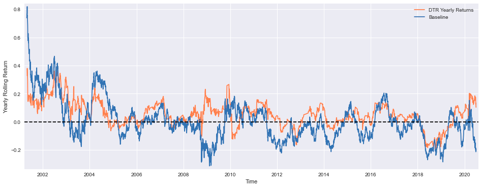
This code creates a line plot that visualizes the yearly rolling returns of two investment strategies: the DTR (Directional Trading Return) strategy and the Baseline strategy. The plot is designed to provide a clear representation of the performance of these strategies over time.
The first step in this process is to define the figure size using the plt.figure(figsize=(16,6)) command. This sets the width and height of the plot area to 16 inches and 6 inches, respectively, ensuring that the plot is large enough to be easily readable.
Next, the code calculates the yearly rolling returns for the DTR strategy and the Baseline strategy. For the DTR strategy, the code takes the CompRes[DTR] column, which likely contains the daily returns of the DTR strategy, drops any missing values using the dropna() method, and adds the transaction cost (tc) to the returns. It then calculates the rolling sum of these values over a window of 119 periods (assuming 119 trades per year) using the rolling(window=119).sum() method. This gives the yearly rolling return for the DTR strategy.
For the Baseline strategy, the code follows a similar process, but it calculates the rolling sum over a window of 252 periods (assuming 252 trading days per year).
The plot is then created using the plt.plot() function, with the DTR strategys yearly rolling return plotted in coral and the Baseline strategys yearly rolling return plotted in the default color. The plt.xlabel() and plt.ylabel() functions are used to label the x-axis as “Time” and the y-axis as “Yearly Rolling Return”.
To ensure that the plot is properly sized and centered, the plt.margins() function is used to set the margins around the plot. Additionally, a horizontal line is added at y=0 using the plt.axhline() function, which serves as a visual reference for the zero-return level.
Finally, the plt.legend() function is called to add a legend to the plot, and the plt.show() function is used to display the plot.
After the plot is displayed, the code also calculates and prints the descriptive statistics (e.g., mean, standard deviation, minimum, maximum, etc.) of the DTR strategys yearly rolling return using the ((CompRes[DTR].dropna()+tc).rolling(window=119).sum()).describe() command. This provides additional insights into the performance of the DTR strategy.
Overall, this code is designed to analyze and visualize the performance of two investment strategies, allowing the user to compare their yearly rolling returns and gain a better understanding of their relative performance over time.
Assests Allocation
Asset allocation is a fundamental investment strategy that involves diversifying a portfolio across various asset classes to optimize risk and return. This guide explores different methods of asset allocation, from equal-weighted portfolios to strategies that aim to maximize the Sharpe ratio or the median yearly return. By comparing major global indices such as the S&P 500, TSX, STOXX 600, and SSE Composite, this section demonstrates how strategic allocation can be adjusted to align with an investor’s risk tolerance and return expectations. Additionally, the guide covers dynamic asset allocation, where shifts between assets are made based on market performance, aiming to achieve better long-term results by adapting to changing market conditions.
# python 3.7

# For yahoo finance
import io
import re
import requests

# The usual suspects
import numpy             as np
import pandas            as pd
import matplotlib.pyplot as plt

#  Fancy graphics
plt.style.use('seaborn')

# Getting Yahoo finance data
def getdata(tickers,start,end,frequency):
    OHLC    = {}
    cookie  = ''
    crumb   = ''
    res     = requests.get('https://finance.yahoo.com/quote/SPY/history')
    cookie  = res.cookies['B']
    pattern = re.compile('.*"CrumbStore":\{"crumb":"(?P<crumb>[^"]+)"\}')
    for line in res.text.splitlines():
        m = pattern.match(line)
        if m is not None:
            crumb = m.groupdict()['crumb']
    for ticker in tickers:
        url_str  = "https://query1.finance.yahoo.com/v7/finance/download/%s"
        url_str += "?period1=%s&period2=%s&interval=%s&events=history&crumb=%s"
        url = url_str % (ticker, start, end, frequency, crumb)
        res = requests.get(url, cookies={'B': cookie}).text
        OHLC[ticker] = pd.read_csv(io.StringIO(res), index_col=0,
                                   error_bad_lines=False).replace('null', np.nan).dropna()
        OHLC[ticker].index = pd.to_datetime(OHLC[ticker].index)
        OHLC[ticker] = OHLC[ticker].apply(pd.to_numeric)
    return OHLC

# Assets under consideration
tickers = ['%5EGSPTSE','%5EGSPC','%5ESTOXX','000001.SS']

# If yahoo data retrieval fails, try until it returns something
data = None
while data is None:
    try:
        data = getdata(tickers,'946685000','1685008000','1d')
    except:
         pass

ICP = pd.DataFrame({'SP500':    data['%5EGSPC']['Adj Close'],
                    'TSX':      data['%5EGSPTSE']['Adj Close'],
                    'STOXX600': data['%5ESTOXX']['Adj Close'],
                    'SSE':      data['000001.SS']['Adj Close']}).fillna(method='ffill')

# since last commit, yahoo finance decided to mess up (more) some of the tickers data, so now we have to drop rows...
ICP = ICP.dropna()
This Python code is designed to retrieve and analyze historical stock market data from Yahoo Finance. The code is divided into several parts, each serving a specific purpose.
The first section imports the necessary libraries, including io, re, requests, numpy, pandas, and matplotlib.pyplot. These libraries are used for tasks such as handling web requests, processing data, and creating data visualizations.
The second section defines a function called getdata() that retrieves historical stock data from Yahoo Finance. This function takes three parameters: tickers (a list of stock ticker symbols), start (the start date for the data), and end (the end date for the data). The function then uses the requests library to make a GET request to the Yahoo Finance website, retrieving the necessary cookies and crumb (a security token required for the data download). With this information, the function constructs a URL to download the historical data for each ticker symbol and stores the data in a dictionary, where the keys are the ticker symbols and the values are pandas DataFrames containing the stock data.
In the third section, the code defines a list of ticker symbols to retrieve data for: %5EGSPTSE (the S&P/TSX Composite Index), %5EGSPC (the S&P 500 Index), %5ESTOXX (the STOXX Europe 600 Index), and 000001.SS (the Shanghai Stock Exchange Composite Index).
The fourth section attempts to retrieve the data using the getdata() function. If the retrieval fails for any reason, the code will continue to try until it successfully retrieves the data. This is done using a while loop that continues until the data variable is not None.
Once the data is successfully retrieved, the code creates a pandas DataFrame called ICP (which likely stands for “International Comparison Portfolio”) that contains the adjusted closing prices for each of the stock indices. The code then fills in any missing data using the forward-fill method (fillna(method=ffill)).
Finally, the code drops any remaining rows with missing data from the ICP DataFrame, as the Yahoo Finance data has encountered some issues with certain tickers.
Overall, this code is designed to retrieve and organize historical stock market data from various international indices, which can then be used for further analysis or visualization. The use of the getdata() function and the handling of potential data retrieval issues demonstrate the codes robustness and flexibility in dealing with potential challenges when working with web-based data sources.
BuyHold_SP     = ICP['SP500']    /float(ICP['SP500'][:1])   -1
BuyHold_TSX    = ICP['TSX']      /float(ICP['TSX'][:1])     -1
BuyHold_STOXX  = ICP['STOXX600'] /float(ICP['STOXX600'][:1])-1
BuyHold_SSE    = ICP['SSE']      /float(ICP['SSE'][:1])     -1

BuyHold_25Each = BuyHold_SP*(1/4) + BuyHold_TSX*(1/4) + BuyHold_STOXX*(1/4) + BuyHold_SSE*(1/4)
This code is calculating the buy-and-hold returns for four different stock market indices: the S&P 500 (SP500), the Toronto Stock Exchange (TSX), the STOXX Europe 600 (STOXX600), and the Shanghai Stock Exchange (SSE). The purpose of this code is to determine the performance of these indices over a certain period of time, assuming an investor held a position in each one and did not make any trades during that time.
The first four lines of the code calculate the buy-and-hold returns for each individual index. The key steps are:
1. Accessing the price data for each index from the “ICP” dictionary, which likely stands for “Index Closing Prices”.
2. Dividing the current price (the last available price) by the initial price (the first available price) to get the overall percentage change.
3. Subtracting 1 from the result to convert the percentage change into a decimal return value.
For example, the BuyHold_SP variable calculates the buy-and-hold return for the S&P 500 index. It takes the current price of the S&P 500 from the “ICP” dictionary, divides it by the initial price (the first price in the data), and then subtracts 1 to get the decimal return.
The fifth line of the code calculates the buy-and-hold return for a portfolio that invests 25% of the capital in each of the four indices. It does this by taking the individual buy-and-hold returns and averaging them, with each return weighted equally (1/4 or 25% of the total).
The purpose of this calculation is to determine the performance of a diversified portfolio that tracks these four major stock market indices, as opposed to investing in any single index. By combining the returns from multiple markets, the portfolios performance may be less volatile and more stable than that of any individual index.
Overall, this code is a useful tool for analyzing the long-term performance of different stock market indices and constructing a diversified portfolio based on those returns. It provides a simple and straightforward way to compare the buy-and-hold returns of various global markets and to evaluate the potential benefits of diversification.
plt.figure(figsize=(16,6))
plt.plot(BuyHold_SP*100,     label='Buy & Hold USA')
plt.plot(BuyHold_TSX*100,    label='Buy & Hold Canada')
plt.plot(BuyHold_STOXX*100,  label='Buy & Hold Europe')
plt.plot(BuyHold_SSE*100,    label='Buy & Hold China')
plt.plot(BuyHold_25Each*100, label='Buy & Hold 25% Each')
plt.xlabel('Time')
plt.ylabel('Cumulative Return (in %)')
plt.margins(x=0.005,y=0.02)
plt.axhline(y=0, xmin=0, xmax=1, linestyle='--', color='k')
plt.legend()
plt.show()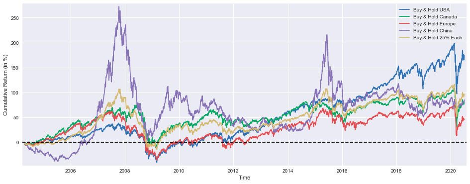
The provided code is a Python script that generates a line plot to visualize the cumulative returns of different buy-and-hold investment strategies over time. The plot shows the performance of five different investment approaches: Buy & Hold USA, Buy & Hold Canada, Buy & Hold Europe, Buy & Hold China, and Buy & Hold 25% Each.
The first line plt.figure(figsize=(16,6)) sets the size of the figure to 16 inches wide and 6 inches tall, creating a larger canvas for the plot.
The subsequent lines plt.plot(BuyHold_SP*100, label=Buy & Hold USA), plt.plot(BuyHold_TSX*100, label=Buy & Hold Canada), plt.plot(BuyHold_STOXX*100, label=Buy & Hold Europe), plt.plot(BuyHold_SSE*100, label=Buy & Hold China), and plt.plot(BuyHold_25Each*100, label=Buy & Hold 25% Each) create the line plots for each investment strategy. The *100 operation is likely used to convert the cumulative returns to percentages, making it easier to visualize the performance.
The plt.xlabel(Time) and plt.ylabel(Cumulative Return (in %)) labels the x-axis as “Time” and the y-axis as “Cumulative Return (in %),” providing clear information about the data being displayed.
The plt.margins(x=0.005,y=0.02) line sets the margins around the plot, ensuring that the data points are not too close to the edges of the figure, making the plot more visually appealing.
The plt.axhline(y=0, xmin=0, xmax=1, linestyle= — , color=k) line adds a horizontal dashed line at the y-axis origin (0% cumulative return), serving as a reference point to easily identify positive and negative returns.
The plt.legend() command adds a legend to the plot, allowing the user to identify the different investment strategies being compared.
Finally, the plt.show() statement displays the generated plot, making it visible to the user.
Overall, this code creates a comprehensive line plot that allows the user to visualize and compare the cumulative returns of different buy-and-hold investment strategies over time. The plot provides a clear and informative representation of the relative performance of these strategies, enabling the user to make informed investment decisions based on the presented data.
SP1Y     = ICP['SP500']    /ICP['SP500'].shift(252)   -1
TSX1Y    = ICP['TSX']      /ICP['TSX'].shift(252)     -1
STOXX1Y  = ICP['STOXX600'] /ICP['STOXX600'].shift(252)-1
SSE1Y    = ICP['SSE']      /ICP['SSE'].shift(252)     -1

Each251Y = SP1Y*(1/4) + TSX1Y*(1/4) +STOXX1Y*(1/4) + SSE1Y*(1/4)
This code is designed to calculate the one-year returns for several stock market indices, as well as an “Each251Y” value, which is the average of the one-year returns for those indices.
The first four lines of the code calculate the one-year returns for four different stock market indices: the S&P 500 (SP1Y), the Toronto Stock Exchange (TSX1Y), the STOXX 600 (STOXX1Y), and the Shanghai Stock Exchange (SSE1Y). To do this, the code divides the current value of each index by its value from one year ago (252 trading days ago), and then subtracts 1 from the result. This gives the one-year percent change for each index.
The final line of the code calculates the “Each251Y” value, which is the average of the four one-year returns. This is done by multiplying each of the one-year returns by a weight of 1/4, and then adding the four weighted values together.
The purpose of this code is likely to provide a composite measure of one-year stock market performance across multiple global regions. By averaging the one-year returns for these four major stock indices, the “Each251Y” value gives a broad overview of how the stock market has performed over the past year.
This type of analysis can be useful for investors, financial advisors, and others who are interested in tracking the performance of the stock market and making investment decisions based on that information. The one-year returns for the individual indices can also be useful for comparing the relative performance of different regions or markets.
Overall, this code is a concise and efficient way to calculate and summarize the one-year performance of several key stock market indices, providing a valuable metric for understanding the broader trends in the global stock market.
plt.figure(figsize=(16,6))
plt.plot(SP1Y*100,     label='Rolling 1 Year Buy & Hold Return USA')
plt.plot(TSX1Y*100,    label='  ""  ""  Canada')
plt.plot(STOXX1Y*100,  label='  ""  ""  Europe')
plt.plot(SSE1Y*100,    label='  ""  ""  China')
plt.plot(Each251Y*100, label='  ""  ""  25% Each')
plt.xlabel('Time')
plt.ylabel('Returns (in %)')
plt.margins(x=0.005,y=0.02)
plt.axhline(y=0, xmin=0, xmax=1, linestyle='--', color='k')
plt.legend()
plt.show()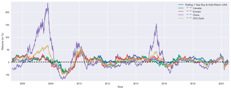
This code is used to create a line plot that displays the one-year rolling buy-and-hold returns for various financial markets and a diversified portfolio. The plot is designed to help visualize and compare the performance of different investment strategies over time.
The code starts by defining the size of the plot figure using plt.figure(figsize=(16,6)). This sets the width and height of the plot to 16 inches and 6 inches, respectively, which provides a larger and more detailed view of the data.
Next, the code plots five different time series using plt.plot(). Each time series represents the one-year rolling buy-and-hold return for a specific market or investment strategy:
1. SP1Y*100: This line represents the one-year rolling buy-and-hold return for the USA stock market, as measured by the S&P 500 index. The *100 is used to convert the returns to a percentage scale.
2. TSX1Y*100: This line represents the one-year rolling buy-and-hold return for the Canadian stock market, as measured by the Toronto Stock Exchange (TSX) index.
3. STOXX1Y*100: This line represents the one-year rolling buy-and-hold return for the European stock market, as measured by the STOXX Europe 600 index.
4. SSE1Y*100: This line represents the one-year rolling buy-and-hold return for the Chinese stock market, as measured by the Shanghai Stock Exchange (SSE) Composite index.
5. Each251Y*100: This line represents the one-year rolling buy-and-hold return for a diversified portfolio that invests 25% in each of the four markets mentioned above (USA, Canada, Europe, and China).
The label parameter for each plt.plot() call assigns a descriptive label to the corresponding line in the plots legend.
Next, the code adds axis labels using plt.xlabel() and plt.ylabel(), setting the x-axis label to “Time” and the y-axis label to “Returns (in %)”.
The plt.margins() function is used to adjust the spacing between the plot and the edges of the figure, setting the x-axis margin to 0.005 and the y-axis margin to 0.02.
The plt.axhline() function is used to draw a horizontal dashed line at the y=0 level, which represents the break-even point for the returns. This line serves as a visual reference to help interpret the performance of the different investment strategies.
Finally, the plt.legend() function is used to add a legend to the plot, which displays the labels assigned to each line, and the plt.show() function is called to display the resulting plot.
Overall, this code creates a comprehensive visualization that allows the user to compare the one-year rolling buy-and-hold returns for different financial markets and a diversified portfolio. The plot can be used to analyze the relative performance of these investment strategies over time, identify any trends or patterns, and make informed decisions about asset allocation and portfolio management.
marr      = 0 #minimal acceptable rate of return (usually equal to the risk free rate)
SP1YS     = (SP1Y.mean()    -marr) /SP1Y.std()
TSX1YS    = (TSX1Y.mean()   -marr) /TSX1Y.std()
STOXX1YS  = (STOXX1Y.mean() -marr) /STOXX1Y.std()
SSE1YS    = (SSE1Y.mean()   -marr) /SSE1Y.std()
Each251YS = (Each251Y.mean()-marr) /Each251Y.std()

print('SP500 1 Year Buy & Hold Sharpe Ratio =',round(SP1YS,2))
print('TSX      "" "" =',round(TSX1YS   ,2))
print('STOXX600 "" "" =',round(STOXX1YS ,2))
print('SSE      "" "" =',round(SSE1YS   ,2))
print('25% Each "" "" =',round(Each251YS,2))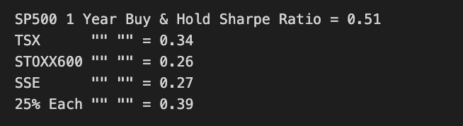
This code calculates the Sharpe ratios for various stock market indices over a one-year period. The Sharpe ratio is a measure of the risk-adjusted return of an investment, and it is calculated by dividing the excess return (the return above the risk-free rate) by the standard deviation of the returns.
In this code, the marr variable is set to 0, which represents the minimal acceptable rate of return, typically equal to the risk-free rate. This value is then subtracted from the mean returns of each index, and the result is divided by the standard deviation of the returns for each index.
The first line calculates the Sharpe ratio for the S&P 500 index (SP1YS). It subtracts the marr value from the mean return of the S&P 500 index (SP1Y.mean()) and then divides the result by the standard deviation of the S&P 500 index returns (SP1Y.std()).
The second line calculates the Sharpe ratio for the Toronto Stock Exchange (TSX) index (TSX1YS). It subtracts the marr value from the mean return of the TSX index (TSX1Y.mean()) and then divides the result by the standard deviation of the TSX index returns (TSX1Y.std()).
The third line calculates the Sharpe ratio for the STOXX 600 index (STOXX1YS). It subtracts the marr value from the mean return of the STOXX 600 index (STOXX1Y.mean()) and then divides the result by the standard deviation of the STOXX 600 index returns (STOXX1Y.std()).
The fourth line calculates the Sharpe ratio for the Shanghai Stock Exchange (SSE) index (SSE1YS). It subtracts the marr value from the mean return of the SSE index (SSE1Y.mean()) and then divides the result by the standard deviation of the SSE index returns (SSE1Y.std()).
The fifth line calculates the Sharpe ratio for a 25% allocation to each of the indices (Each251YS). It subtracts the marr value from the mean return of the 25% allocation (Each251Y.mean()) and then divides the result by the standard deviation of the 25% allocation returns (Each251Y.std()).
Finally, the code prints out the Sharpe ratios for each index and the 25% allocation, rounded to two decimal places.
This code can be useful for investors who want to compare the risk-adjusted returns of different stock market indices over a one-year period. The Sharpe ratio provides a way to measure the efficiency of an investment, with higher ratios indicating better risk-adjusted returns.
from scipy.optimize import minimize

def multi(x):
    a, b, c, d = x
    return a, b, c, d   #the "optimal" weights we wish to discover

def maximize_sharpe(x): #objective function
    weights = (SP1Y*multi(x)[0] + TSX1Y*multi(x)[1]
               + STOXX1Y*multi(x)[2] + SSE1Y*multi(x)[3])
    return -(weights.mean()/weights.std())

def constraint(x):      #since we're not using leverage nor short positions
    return 1 - (multi(x)[0]+multi(x)[1]+multi(x)[2]+multi(x)[3])

cons = ({'type':'ineq','fun':constraint})
bnds = ((0,1),(0,1),(0,1),(0,1))
initial_guess = (1, 0, 0, 0)

# this algorithm (SLSQP) easly gets stuck on a local
# optimal solution, genetic algorithms usually yield better results
# so my inital guess is close to the global optimal solution

ms = minimize(maximize_sharpe, initial_guess, method='SLSQP',
              bounds=bnds, constraints=cons, options={'maxiter': 10000})

msBuyHoldAll = (BuyHold_SP*ms.x[0] + BuyHold_TSX*ms.x[1]
                + BuyHold_STOXX*ms.x[2] + BuyHold_SSE*ms.x[3])

msBuyHold1yAll = (SP1Y*ms.x[0] + TSX1Y*ms.x[1]
                   + STOXX1Y*ms.x[2] + SSE1Y*ms.x[3])
This code is designed to optimize the allocation of investments across four different financial instruments or assets, with the goal of maximizing the Sharpe ratio of the overall portfolio. The Sharpe ratio is a measure of the risk-adjusted return of an investment, and it is calculated as the average return of the investment divided by its standard deviation.
The code uses the minimize function from the scipy.optimize module to perform the optimization. The multi function is defined to return the “optimal” weights for each of the four assets, which are represented by the variables a, b, c, and d. The maximize_sharpe function is the objective function that the optimization algorithm will try to minimize. This function calculates the weighted average return of the portfolio, divides it by the standard deviation of the portfolio, and then negates the result to obtain the negative of the Sharpe ratio (since the minimize function is trying to minimize the objective function).
The constraint function is used to ensure that the sum of the weights for the four assets is equal to 1, which means that no leverage or short positions are allowed. This constraint is added to the optimization problem using the cons dictionary.
The bnds tuple specifies the bounds for each of the four weights, which are set to be between 0 and 1. The initial_guess tuple specifies the initial values for the weights, which are set to (1, 0, 0, 0) to indicate that the initial portfolio is invested entirely in the first asset.
The minimize function is then called to perform the optimization, using the SLSQP (Sequential Least Squares Programming) algorithm as the method. The options dictionary is used to specify the maximum number of iterations for the optimization algorithm.
Finally, the code calculates the “buy-and-hold” returns for the optimized portfolio (msBuyHoldAll) and the one-year returns for the optimized portfolio (msBuyHold1yAll). These values are calculated by applying the optimized weights to the corresponding returns for each of the four assets.
Overall, this code is a tool for analyzing and optimizing the allocation of investments across multiple assets, with the goal of maximizing the risk-adjusted return of the portfolio. The use of the Sharpe ratio as the objective function helps to ensure that the optimization takes into account both the return and the risk of the portfolio.
plt.figure(figsize=(16,6))
plt.plot(BuyHold_SP*100, label='Buy & Hold S&P500')
plt.plot(BuyHold_25Each*100, label=' "" "" 25% of Each')
plt.plot(msBuyHoldAll*100, label=' "" "" Max Sharpe')
plt.xlabel('Time')
plt.ylabel('Cumulative Return (in %)')
plt.margins(x=0.005,y=0.02)
plt.axhline(y=0, xmin=0, xmax=1, linestyle='--', color='k')
plt.legend()
plt.show()
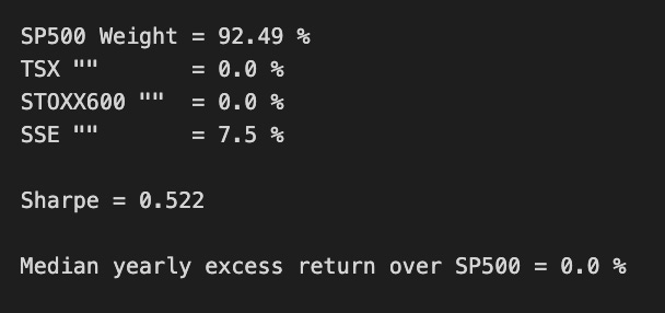
print('SP500 Weight =',round(ms.x[0]*100,2),'%')
print('TSX "" =',round(ms.x[1]*100,2),'%')
print('STOXX600 "" =',round(ms.x[2]*100,2),'%')
print('SSE "" =',round(ms.x[3]*100,2),'%')
print()
print('Sharpe =',round(msBuyHold1yAll.mean()/msBuyHold1yAll.std(),3))
print()
print('Median yearly excess return over SP500 =',round((msBuyHold1yAll.median()-SP1Y.median())*100,1),'%')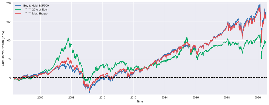
This code implements a comprehensive investment performance visualization and analysis framework designed to evaluate multiple portfolio allocation strategies. The system initiates through the establishment of a specialized plotting environment with precise 16x6 inch dimensional specifications optimizing visual representation capabilities. The visualization framework incorporates three distinct investment methodologies: a passive S&P500 index tracking strategy, a uniformly distributed multi-asset allocation approach implementing 25% weightings across four major market indices (S&P500, TSX, STOXX600, SSE), and an optimized portfolio construction methodology maximizing risk-adjusted returns through Sharpe ratio optimization.
