


Advanced Machine Learning and Deep Learning Techniques for Stock Market Analysis
Advanced Machine Learning and Deep Learning Techniques for Stock Market Analysis
Harnessing Python’s Capabilities for Financial Data Analysis

Download the source code from the link at the end of this article.
In the rapidly evolving world of stock market analysis, the integration of machine learning and deep learning techniques has become increasingly crucial for investors and analysts. This article delves into an advanced approach to analyzing stock market data, utilizing both traditional machine learning models and state-of-the-art deep learning methods. We will explore a comprehensive script that leverages Python’s powerful libraries to extract meaningful insights from stock data, aiming to enhance prediction accuracy and decision-making in trading strategies.
from __future__ import division
import pandas as pd
import numpy as np
import matplotlib.pyplot as plt
from pandas.plotting import scatter_matrix
import pandas as pd
from sklearn.model_selection import train_test_split, cross_val_score
from sklearn.ensemble import RandomForestClassifier
from sklearn import datasets
from sklearn import svm,neighbors
from sklearn.model_selection import cross_val_score
from sklearn.preprocessing import RobustScaler, MinMaxScaler
from sklearn import metrics
from sklearn.model_selection import cross_val_predict
from sklearn import model_selection
from sklearn.metrics import classification_report
from sklearn.metrics import confusion_matrix
from sklearn.metrics import accuracy_score, mean_squared_error
from sklearn.tree import DecisionTreeClassifier
from sklearn.neighbors import KNeighborsClassifier
from sklearn.naive_bayes import GaussianNB
from sklearn.svm import SVC
from tensorflow import keras
from keras.models import Sequential
from keras.layers import Dense, Dropout, LSTM, Conv1D
from keras.callbacks import ReduceLROnPlateau
Firstly, the script begins by preparing for compatibility between Python 2 and Python 3, ensuring that division will work as expected in Python 3. It imports pandas, a library for data structures and data analysis, and numpy, used for numerical computations. Additionally, matplotlib’s pyplot is imported for data visualization, allowing the creation of plots and graphs. The pandas library is re-imported, which seems redundant as it was already imported earlier. Following this, a scatter matrix is imported, used to visualize pair-wise relationships and distributions of variables within a DataFrame.
The script then includes imports from scikit-learn, a machine learning library, including various machine learning models such as RandomForestClassifier, SVC (Support Vector Classifier), KNeighborsClassifier, DecisionTreeClassifier, and GaussianNB (Naive Bayes). These imports suggest the code may involve training and evaluating one or more of these models. Utilities for splitting data into training and test sets, cross-validation, and preprocessing are imported, signaling that the data will be prepared and validated using standard machine learning practices.
Moreover, various metrics for model performance evaluation such as classification reports, confusion matrices, accuracy scores, and mean squared error are included, meaning the code likely involves assessing the predictive performance of the models. Finally, imports from TensorFlow and its high-level API, Keras, suggest that the code will also involve constructing neural networks. Specific elements like Sequential (for creating a linear stack of neural network layers), Dense (for fully connected layers), Dropout (to prevent overfitting), LSTM and Conv1D (different types of neural network layers), as well as a learning rate scheduler (ReduceLROnPlateau) hint at more complex models and training procedures that may be part of the script’s functionality.
Loading The Dataset
"""The CSV file we are using here contains 10 year details
of 5 stocks - RELIANCE, HDFC, TCS, ITC and INFOSYS """

df = pd.read_csv("/content/stock_data.csv")
df.head()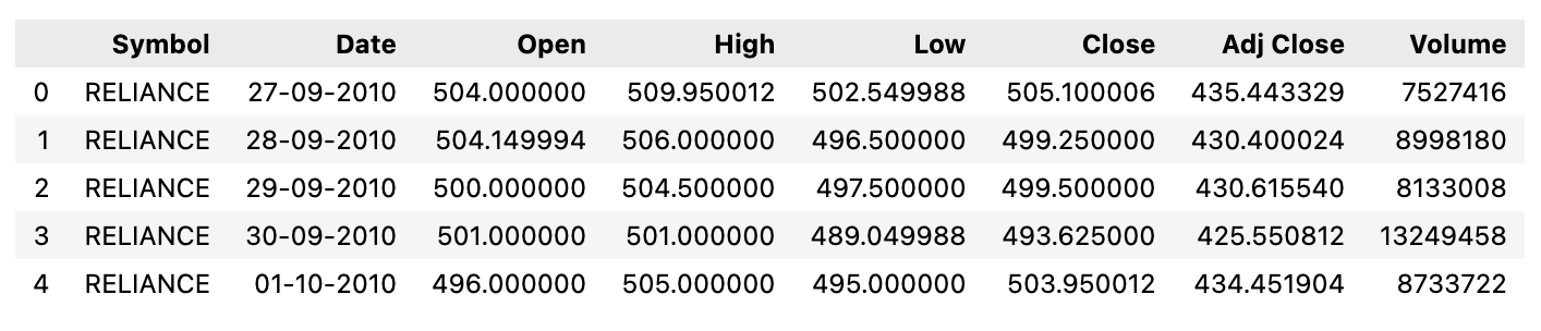
The dataset is in the form of a CSV file, a common format for storing tabular data, containing information related to the stock market. It includes details from a ten-year period for five different stocks: RELIANCE, HDFC, TCS, ITC, and INFOSYS, notable companies in India with significant trading volume on the stock exchanges.
The code utilizes the pandas library, an important tool in Python for data manipulation and analysis. By invoking the `read_csv` function from pandas, the script reads the stock market data from the CSV file located at the specified file path. Once the data is read into the Python environment, it is stored in a DataFrame. A DataFrame is a two-dimensional, size-mutable, and potentially heterogeneous tabular data structure in pandas, with labeled axes (rows and columns).
After loading the data, the script then calls the `head()` method on the DataFrame. This method is used to retrieve and display the first few rows from the DataFrame. By default, `head()` returns the first five rows, providing a quick overview of the data, including the column names and some values for each of the five stocks mentioned. This snapshot is useful for gaining an initial understanding of the dataset’s structure and contents before proceeding with more in-depth data analysis or manipulation tasks.
Feature Extraction
"""
The individual stocks data consists of Date, Open,
High, Low, Close and Volume. Using this data we calculated
our features based on various technical indicators
"""

df['signal'] = 0.0
df['short_mavg'] = df['Close'].rolling(window=30, min_periods=1, center=False).mean()
df['long_mavg'] = df['Close'].rolling(window=120, min_periods=1, center=False).mean()
df['signal'] = np.where(df['short_mavg'] > df['long_mavg'], 1.0, 0.0)
The dataframe includes columns for various pieces of information for a stock on any given day, like the date, the opening price, highest price of the day, lowest price of the day, closing price, and the volume of stocks traded. The code is focused on creating new features within this dataframe that are derived from the existing data, particularly from the ‘Close’ price data, which is presumably the price at which the stock closed on each trading day.
These new features are based on technical indicators that are often used by traders and analysts to make decisions about buying and selling stocks. Firstly, the script sets up a new column labeled ‘signal’, initializing it to zero. This is a placeholder for what will become a trade signal based on the conditions determined by the technical indicators.
Then, the script calculates two separate moving averages of the closing prices, each over different window sizes. A short-term moving average is computed over a window of the last 30 days, and similarly, a long-term moving average is computed over a larger window of the last 120 days. A moving average is a commonly used indicator in stock trading that helps to smooth out price data over a given time period to better identify trends. The short-term average is more responsive to recent price changes, whereas the long-term average is less sensitive and indicates the longer-term trend.
Finally, the script generates a trading ‘signal’ based on a comparison between these two moving averages. Whenever the short-term moving average is greater than the long-term moving average, it assigns a value of 1.0 to the ‘signal’ column for that particular day, suggesting a potential “buy” signal. Conversely, when the short-term average is not greater than the long-term average, the ‘signal’ remains 0.0, which is possibly interpreted as a “hold” or “sell” signal, depending on the strategy used by the trader.
This technique is based on a common trading strategy known as the “moving average crossover”, where traders look for points in time where a short-term moving average crosses above a long-term moving average as an indicator of upward momentum, suggesting it might be a good time to buy.
def EMA(df, n):
    """ Function to calculate exponential moving average"""
    EMA = pd.Series(df['Close'].ewm(span=n, min_periods=n).mean(), name='EMA_' + str(n))
    return EMA

df['EMA21'] = EMA(df, 21)
df['EMA63'] = EMA(df, 63)
df['EMA252'] = EMA(df, 252)
df.tail()
The code defines a function to compute the Exponential Moving Average (EMA) of a financial asset’s closing prices over a given period. The EMA is a type of weighted moving average that places a greater emphasis on the most recent prices, and is commonly used by traders and analysts to identify trends in the price data of stocks, commodities, or other traded instruments. The function takes in a dataframe and a time period specified by ’n’, then calculates the EMA for the ‘Close’ price column in that dataframe. It uses a built-in function specifically designed for this purpose, which is capable of handling the complex calculation that defines the EMA.
The function applies the EMA calculation starting after ’n’ periods to ensure the calculation has enough data points. Once computed, this EMA series is named using the period ’n’ to distinguish it among potentially many EMAs calculated over different periods. After defining the function, the code proceeds to add three EMAs to the original dataframe, each with different time periods: 21, 63, and 252 days.
These periods might represent one month, one quarter, and one year in trading days, assuming approximately 21 trading days in a month. Each of these EMAs is stored as a new column in the dataframe, and the names of these columns reflect the periods over which they were calculated.
def ROC(df, n):
    """Function to calculate Rate of Change"""
    M = df.diff(n - 1)
    N = df.shift(n - 1)
    ROC = pd.Series(((M / N) * 100), name = 'ROC_' + str(n))
    return ROC

df['ROC21'] = ROC(df['Close'], 21)
df['ROC63'] = ROC(df['Close'], 63)
This function takes a dataframe and a numerical value as inputs. When this function is called, it first calculates the difference between the current price and the price ’n’ periods ago. ’n’ represents the period specified by the user. It then takes the price ’n’ periods ago and calculates the ratio of the price change to the price ’n’ periods ago, multiplies it by 100 to convert it to a percentage, and creates a new pandas Series with this information.
The name of this new Series is set to include ‘ROC_’ followed by the period number to distinguish the calculated ROC for different periods. The function then returns the Series it has created. After the function definition, the code proceeds to create two new columns in the dataframe that was provided as an input. For each column, it calls the ROC function, once with a period of 21 and once with a period of 63, using the ‘Close’ prices from the dataframe.
These new columns are named ‘ROC21’ and ‘ROC63’, respectively, indicating the ROC calculated over 21 and 63 periods. This addition of new columns effectively appends the 21-day and 63-day Rate of Change indicators to the dataframe for further analysis or visualization.
def MOM(df, n):
    """Function to calculate price momentum"""
    MOM = pd.Series(df.diff(n), name='Momentum_' + str(n))
    return MOM
df['MOM21'] = MOM(df['Close'], 21)
df['MOM63'] = MOM(df['Close'], 63)
This function, named MOM, takes two parameters: a dataframe that contains financial data, such as stock prices, and a number ’n’ that represents the number of periods over which to calculate the momentum. The function works by taking the difference between the current closing price and the closing price ’n’ periods ago. For example, if ’n’ is 21, it computes the difference between today’s closing price and the closing price 21 days ago.
The result of this calculation is assigned to a new series with a name indicating that it represents momentum calculated over ’n’ periods. After defining the function, the code applies it twice to the closing price data in the dataframe. The closing price data is assumed to be a column labeled ‘Close’ within the dataframe. The function is first used to calculate 21-day momentum, storing the result in the dataframe with a new column labeled ‘MOM21’. Afterwards, the same function is used again to calculate the 63-day momentum, creating another column labeled ‘MOM63’.
def RSI(series, period):
    """Function to calculate Relative Strength Index"""
    delta = series.diff().dropna()
    u = delta * 0
    d = u.copy()
    u[delta > 0] = delta[delta > 0]
    d[delta < 0] = -delta[delta < 0]

    #first value is sum of avg gains
    u[u.index[period-1]] = np.mean( u[:period] )
    u = u.drop(u.index[:(period-1)])

    #first value is sum of avg losses
    d[d.index[period-1]] = np.mean( d[:period] )
    d = d.drop(d.index[:(period-1)])
    rs = u.rolling(period-1).mean() / d.rolling(period-1).mean()
    return 100 - 100 / (1 + rs)

df['RSI21'] = RSI(df['Close'], 21)
df['RSI63'] = RSI(df['Close'], 63)
df['RSI252'] = RSI(df['Close'], 252)
The RSI is a type of momentum indicator that measures the magnitude of recent price changes to evaluate overbought or oversold conditions in the price of a stock or other asset. The function works by taking in a series of price data along with a period that represents the time frame for which the RSI is to be calculated. Initially, the code calculates the difference between consecutive prices to find out how much the price has changed each day.
It then classifies these differences into gains and losses, distinguishing the days where the price went up from those where it went down. In the next step, it calculates the average gains and average losses over the specified period. This involves modifying the initial gains and losses data, ensuring that the first value is the average of gains or losses over the period, and discarding the rest of the data that falls before this period. Once the average gains and losses have been established, the function proceeds to calculate the relative strength (RS) by dividing the average gains by the average losses.
This RS value is then used to calculate the RSI, which normalizes the momentum into a scale of 0 to 100. The RSI value helps traders to identify whether an asset is potentially overbought, usually indicated by a high RSI, or oversold, indicated by a low RSI. Towards the end of the code snippet, the function is applied to calculate the RSI values of closing prices over different periods (like 21, 63 and 252 days) for a dataset. These RSI values are then stored within the original dataset as new columns, allowing for further analysis or trading decisions. Each of the columns generated gives the RSI reading across different time frames, providing a depth of insight into the momentum of price changes over short, medium, and long terms.
#calculation of stochastic osillator.
def STOK(close, low, high, n):
    """Function to calculate Fast Stochastic Oscillator"""
    STOK = ((close - low.rolling(n).min()) / (high.rolling(n).max() - low.rolling(n).min())) * 100
    return STOK

def STOD(close, low, high, n):
    """Function to calculate Slow Stochastic Oscillator
     (3-period moving average of STOK) """
    STOK = ((close - low.rolling(n).min()) / (high.rolling(n).max() - low.rolling(n).min())) * 100
    STOD = STOK.rolling(3).mean()
    return STOD

df['%K21'] = STOK(df['Close'], df['Low'], df['High'], 21)
df['%D21'] = STOD(df['Close'], df['Low'], df['High'], 21)
df['%K63'] = STOK(df['Close'], df['Low'], df['High'], 63)
df['%D63'] = STOD(df['Close'], df['Low'], df['High'], 63)
df['%K252'] = STOK(df['Close'], df['Low'], df['High'], 252)
df['%D252'] = STOD(df['Close'], df['Low'], df['High'], 252)
df.tail()
The Fast Stochastic Oscillator and the Slow Stochastic Oscillator are the two versions of the oscillator that are calculated by the functions. The Fast Stochastic Oscillator, computed by the `STOK` function, compares the current closing price of a stock to the range of its highs and lows over a certain period of time, defined by ’n’. By subtracting the lowest low from the current closing price, and then dividing this by the difference between the highest high and the lowest low within that period, and finally multiplying the fraction by 100, the resulting value is a percentage that indicates where the close is in relation to the range. This value is referred to as the %K line.
The Slow Stochastic Oscillator is an average of the Fast Stochastic values, which aims to smooth out the results and provide a more reliable signal. This is calculated by the `STOD` function, which specifically takes the rolling 3-period moving average of the Fast Stochastic Oscillator’s values. The code applies these functions to a dataframe (presumably containing stock market data) for three different periods: 21, 63, and 252 days. This results in six new columns within the dataframe, containing the fast (%K) and slow (%D) stochastic values for each of these three timeframes.