

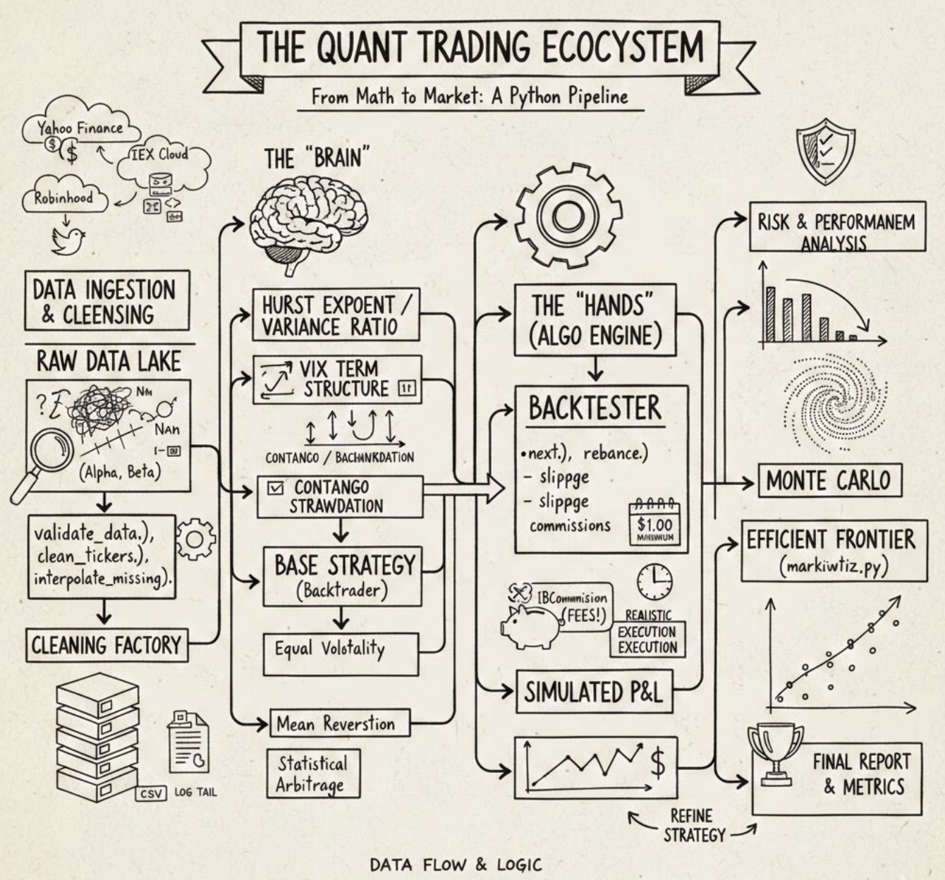
Advanced Quant Trading: Mastering Mean Reversion and Volatility Regimes
A Data-Driven Framework for Institutional-Grade Quant Trading Performance

Download Source code using the button at the end of this article:
In the fast-evolving world of algorithmic finance, the line between a profitable strategy and a failed experiment often lies in the quality of the underlying framework. This article provides a comprehensive deep dive into a production-grade Quant Trading ecosystem, built from the ground up using Python and Backtrader. Whether you are an aspiring quantitative researcher or an experienced developer, you will explore the full lifecycle of systematic trading — ranging from multi-source data ingestion (Yahoo Finance, IEX, and Robinhood) to advanced statistical validation using Hurst Exponents and Variance Ratios. Readers can expect to find a modular architecture designed for real-world robustness, featuring custom risk analyzers like the Sortino Ratio, sophisticated rebalancing logic, and automated data cleaning routines. By the end of this guide, you will learn how to bridge the gap between abstract mathematical theory and a functional execution engine, gaining the tools necessary to build, backtest, and refine institutional-quality Quant Trading strategies with scientific rigor and engineering precision.
# file path: backtest/run.py
import datetime
import os.path
import argparse
import importlib
import dateutil.parser
import pandas as pd
import numpy as np
import backtrader as bt
from backtrader import TimeFrame
from .util import commission, observers, analyzers
from .util import universe as universe_util
The import list assembles standard libraries, numeric/data tools, the backtesting engine, and our local utilities that the run entry point needs to orchestrate a backtest. datetime and os.path are used for handling date arithmetic and filesystem paths when locating price and VIX files; argparse and importlib enable command-line argument parsing and dynamic loading of a strategy module at runtime so the runner can invoke different strategies without hard-coding them; dateutil.parser is used to robustly convert user-supplied date strings into datetime objects for configuration of the backtest window. pandas and numpy provide the DataFrame/array operations used to shape raw market data and VIX term-structure series before they are passed into the engine. backtrader and the TimeFrame symbol are pulled in because the backtest runner constructs and configures a backtrader engine instance and needs timeframe semantics for resampling or feeding data. The local utilities commission, observers, and analyzers supply project-specific backtrader extensions for trade cost modeling, runtime observability, and performance measurement (including the Sortino analysis invoked later), while universe as universe_util centralizes ticker normalization and universe-group logic used to prepare the list of symbols the runner will request. This file’s imports mirror patterns elsewhere in the project—backtrader is a core dependency imported in multiple modules, and the util pieces match the same responsibilities seen in other files, with a small namespacing variance where some modules import those utilities from the package root while the runner references them through the util subpackage.
# file path: backtest/run.py
def clean_tickers(tickers, start, end):
    data_path = os.path.join(os.path.dirname(__file__), ‘../data/price/’)
    out_tickers = []
    for ticker in tickers:
        d = pd.read_csv(data_path + ticker + ‘.csv’, index_col=0, parse_dates=True)
        if not (d.tail(1).index[0] < start or
                d.head(1).index[0] > end):
            out_tickers.append(ticker)
        else:
            print(’Data out of date range:’, ticker)
    return out_tickers
clean_tickers is the pre-filter the backtest runner uses to make sure the strategy only receives tickers with on-disk price series that actually overlap the requested backtest window. It computes a data directory relative to the module file, then loops over each ticker and reads its CSV into a pandas DataFrame with the first column as a datetime index. For each loaded series it inspects the earliest and latest timestamps (via head and tail) and applies a simple overlap test: if the series ends before the requested start or begins after the requested end the ticker is reported to the console as out of date range and is excluded; otherwise the ticker is appended to the output list. The function returns that filtered list of tickers. Because clean_tickers performs the date-range check up front, run_strategy downstream will only invoke analysis and plotting on tickers with at least some usable data; any file-read or parse errors are not handled inside clean_tickers and would propagate out.
# file path: tools/log/log.py
import os
from datetime import datetime
The tools logging module needs basic filesystem access and timestamping so it can append and read time-stamped log lines; the two imports supply those capabilities. The os import brings in standard filesystem and path utilities the log, last, and tail helpers use to locate, open, and inspect the log file on disk. Importing the datetime class gives direct access to current timestamps so each log entry is created with an exact time and so recent entries can be identified when tail inspects activity. By contrast, the other import examples you’ve seen in the codebase are intra-package imports that pull the log module or combine log with fin_calc for higher-level functionality; here the module is simply pulling in core standard-library building blocks that enable writing and reading time-stamped files.
# file path: tools/log/log.py
def tail(count=5):
    with open(LOG_FILE_PATH, ‘r’) as f:
        total_lines_wanted = count
        BLOCK_SIZE = 1024
        f.seek(0, 2)
        block_end_byte = f.tell()
        lines_to_go = total_lines_wanted
        block_number = -1
        blocks = []
        while lines_to_go > 0 and block_end_byte > 0:
            if (block_end_byte - BLOCK_SIZE > 0):
                f.seek(block_number*BLOCK_SIZE, 2)
                blocks.append(f.read(BLOCK_SIZE))
            else:
                f.seek(0, 0)
                blocks.append(f.read(block_end_byte))
            lines_found = blocks[-1].count(’\n’)
            lines_to_go -= lines_found
            block_end_byte -= BLOCK_SIZE
            block_number -= 1
        all_read_text = ‘’.join(reversed(blocks))
        for line in all_read_text.splitlines()[-total_lines_wanted:]:
            print(line)
Within the tools package’s simple logging utilities, the tail function reads and prints the last N log lines from the file referenced by LOG_FILE_PATH so clean_tickers can inspect recent activity during cleanup. It opens the log file for text reading, records the requested number of lines and a block size (1 KB), then moves the file cursor to the end to determine the file length. The function then walks backwards through the file in fixed-size blocks: for each iteration it seeks to the next block from the end (using negative block offsets) or, when the remaining bytes are smaller than a block, seeks to the file start and reads the remainder. Each read block is appended to a temporary list and the function counts how many newline characters that block contains to decrement how many more lines it needs. The loop continues until either the requested number of lines has been found or the start of the file is reached. After that it reverses the collected blocks to restore chronological order, joins them into one string, splits into lines, and prints the final requested slice of lines to the console. Control flow covers the happy path of finding enough lines via multiple block reads and the edge case where the entire file is smaller than the requested tail length, in which case the function simply prints whatever lines exist. Conceptually this implements a backward-chunk-reading pattern to avoid loading the whole log file into memory; it differs from the last and get_last_date helpers, which operate in binary mode and search for a single trailing newline by stepping backward byte-by-byte.
# file path: backtest/run.py
def run_strategy(strategy, tickers=None, start=’1900-01-01’, end=’2100-01-01’, cash=100000.0,
                 verbose=False, plot=False, plotreturns=False, universe=None, exclude=[],
                 kwargs=None):
    start_date = dateutil.parser.isoparse(start)
    end_date = dateutil.parser.isoparse(end)
    tickers = tickers if (tickers or universe) else [’SPY’]
    if universe:
        u = universe_util.get(universe)()
        tickers = [a for a in u.assets if a not in exclude]
    tickers = clean_tickers(tickers, start_date, end_date)
    module_path = f’.algos.{strategy}’
    module = importlib.import_module(module_path, ‘backtest’)
    strategy = getattr(module, strategy)
    cerebro = bt.Cerebro(
        stdstats=not plotreturns,
        cheat_on_open=strategy.params.cheat_on_open
    )
    cerebro.addstrategy(strategy, verbose=verbose)
    for ticker in tickers:
        datapath = os.path.join(os.path.dirname(__file__), f’../data/price/{ticker}.csv’)
        data = bt.feeds.YahooFinanceCSVData(
            dataname=datapath,
            fromdate=start_date,
            todate=end_date,
            reverse=False,
            adjclose=False,
            plot=not plotreturns)
        cerebro.adddata(data)
    cerebro.broker.setcash(cash)
    if plotreturns:
        cerebro.addobserver(observers.Value)
    cerebro.addanalyzer(bt.analyzers.SharpeRatio,
                        riskfreerate=strategy.params.riskfreerate,
                        timeframe=TimeFrame.Days,
                        annualize=True)
    cerebro.addanalyzer(analyzers.Sortino,
                        riskfreerate=strategy.params.riskfreerate,
                        timeframe=TimeFrame.Days,
                        annualize=True)
    cerebro.addanalyzer(bt.analyzers.Returns)
    cerebro.addanalyzer(bt.analyzers.DrawDown)
    cerebro.addanalyzer(bt.analyzers.PositionsValue)
    cerebro.addanalyzer(bt.analyzers.GrossLeverage)
    results = cerebro.run(preload=False)
    start_value = cash
    end_value = cerebro.broker.getvalue()
    print(’Starting Portfolio Value:\t{:.2f}’.format(cash))
    print(’Final Portfolio Value:\t\t{:.2f}’.format(end_value))
    drawdown = results[0].analyzers.drawdown.get_analysis()[’max’][’drawdown’]
    cagr = results[0].analyzers.returns.get_analysis()[’rnorm100’]
    sharpe = results[0].analyzers.sharperatio.get_analysis()[’sharperatio’]
    sortino = results[0].analyzers.sortino.get_analysis()[’sortino’]
    positions = results[0].analyzers.positionsvalue.get_analysis()
    avg_positions = np.mean([sum(d != 0.0 for d in i) for i in positions.values()])
    leverage = results[0].analyzers.grossleverage.get_analysis()
    avg_leverage = np.mean([abs(i) for i in leverage.values()])
    sharpe = ‘None’ if sharpe is None else round(sharpe, 5)
    print(’ROI:\t\t{:.2f}%’.format(100.0 * ((end_value / start_value) - 1.0)))
    analyzer_results = []
    analyzer_results.append(’Max Drawdown:\t{:.2f}’.format(drawdown))
    analyzer_results.append(’CAGR:\t\t{:.2f}’.format(cagr))
    analyzer_results.append(’Sharpe:\t\t{}’.format(sharpe))
    analyzer_results.append(’Sortino:\t{:.5f}’.format(sortino))
    analyzer_results.append(’Positions:\t{:.5f}’.format(avg_positions))
    analyzer_results.append(’Leverage:\t{:.5f}’.format(avg_leverage))
    print(’\n’.join(analyzer_results))
    if plot:
        cerebro.plot()
Back in run — continuing with run_strategy, the function orchestrates the end-to-end backtest run by preparing inputs, wiring them into Backtrader, executing the strategy, and summarizing the analyzers. It first turns the start and end strings into datetime objects and decides the ticker universe: if a universe name is provided it resolves that with universe_util.get and filters out any excluded tickers; if no tickers or universe are supplied it falls back to a single default asset. It then calls clean_tickers to validate each ticker’s local CSV price file against the requested date range, so only assets with data inside the window proceed. The strategy implementation is imported dynamically using importlib and the class object is retrieved so the test can instantiate the exact algorithm requested. A Backtrader Cerebro engine is created with standard statistics enabled or disabled depending on whether plotreturns is requested, and the cheat-on-open behavior is set from the strategy’s parameters
# file path: tools/plot.py
import os
import argparse
from datetime import datetime
import numpy as np
import pandas as pd
from pandas.plotting import register_matplotlib_converters
from matplotlib import pyplot as plt
The file brings in standard and third-party libraries needed to turn time-indexed strategy output into numerical results and visualizations: os is used for filesystem work such as creating or resolving paths and saving plot files; argparse provides CLI parsing so the plotting utilities can be invoked or parameterized from a command line; datetime.datetime supplies timestamp parsing and construction for axis labels and for converting string dates into temporal objects; numpy (aliased as np) supplies the vectorized numeric operations used to compute log returns and other array math; pandas (aliased as pd) is used to manipulate time-series data coming from Strategy.log, to hold the DataFrame/Series objects that feed the plots; pandas.plotting.register_matplotlib_converters ensures pandas datetime indices are correctly handled by the plotting backend so time axes render properly; and matplotlib.pyplot (aliased as plt) is the plotting API used to draw, format, and persist the performance charts. These imports match the project’s pattern where many modules pull in os, argparse, pandas and numpy for CLI-driven data workflows, but plot adds the datetime converter and pyplot imports specific to its standalone role of rendering time-series performance visuals (where some other modules import date instead of datetime or domain libraries like pypfopt for optimization).
# file path: tools/plot.py
def plot(data, plot_returns=False):
    if plot_returns:
        data = _log_returns(data)
    plt.clf()
    for y in data:
        print(y.name)
        plt.plot(y, label=y.name)
    plt.legend()
    plt.tight_layout()
    plt.show()
When run_strategy hands a collection of time series into plot, plot first decides whether those series should be converted into cumulative log returns by delegating to _log_returns; if plot_returns is True, _log_returns transforms each series by taking the log, differencing to get period returns, forcing the first value to zero, and then forming a cumulative return series. After that optional transformation, plot clears the current matplotlib figure, then iterates over the supplied series (it expects iterable objects like pandas Series that carry a name), prints each series name to the console so you can see which trace is being rendered, and plots each trace on the same axes. When all series are drawn it enables the legend, tightens the layout to avoid clipping, and displays the figure. The control flow is a simple guard on plot_returns followed by a loop over data; its observable side effects are console output for each series name and the interactive plot window used to visualize raw price series or cumulative log-return performance for strategy comparison.
# file path: tools/plot.py
def _log_returns(data):
    log_d = []
    for d in data:
        r = np.log(d).diff()
        r.iloc[0] = 0.0
        r = np.cumprod(r + 1) - 1
        log_d.append(r)
    return log_d
In the backtester pipeline this helper prepares series for the performance plots by turning each incoming price-like series into a compounded return curve that the plot routine can draw. For each series in the provided iterable it takes the natural-log transform and differences it to get period log-returns, replaces the first-period result with zero to avoid a missing value at the start, then treats those period values as one-plus-returns and takes a cumulative product and subtracts one to produce a cumulative, compounded return series; each resulting series is collected and returned in the same order as the input. The loop is the simple accumulator that implements that sequence for every asset/strategy series you pass in; plot calls this when plot_returns is requested and then graphs each returned series (using the series name as the label). Compared with the standalone log_returns helper, which only returns the raw log-differences trimmed of the initial NaN, _log_returns produces ready-to-plot cumulative return curves anchored at zero.
# file path: backtest/algos/BaseStrategy.py
import backtrader as bt
This file pulls in the external backtrader library so the BaseStrategy implementation can rely on backtrader’s primitives — lifecycle hooks, data feed and broker interfaces, order and notification objects, and the event-driven run loop — rather than reimplementing those concerns. In the context of the algo-trader-master_cleaned architecture, that single external import ties the project’s strategy layer into the backtesting engine: BaseStrategy will extend or call into backtrader types to receive ticks/candles, submit orders, and handle order callbacks. Other modules in the codebase follow the opposite direction: they import BaseStrategy (sometimes aliased as base) or import BaseStrategy together with concrete algorithms like BuyAndHold and CrossOver to assemble or register strategies for backtests. In short, this import brings the external framework into the strategy base so internal strategy classes can plug into the backtesting lifecycle, while the rest of the project imports the resulting BaseStrategy to build higher-level algorithm compositions.
# file path: backtest/algos/BaseStrategy.py
    def log(self, txt, date=None):
        if self.verbose:
            date = date or self.data.datetime.date(0)
            print(’{}, {}’.format(date.isoformat(), txt))
Strategy.log is the small, centralized diagnostic helper the Strategy base class uses to emit human-readable lifecycle messages to the console when a backtest is running. It honors the verbose flag that Strategy.init copies from the strategy parameters, so logging only happens when the strategy was configured to be chatty. When called it either uses the date the caller provided or, if none was supplied, pulls the current bar date from the active data feed via the strategy’s primary data datetime accessor; it then prints a single line combining the ISO-formatted date and the textual message. Most concrete strategies and the notify_order handler call Strategy.log to report events like order creation, fills, costs and rejections, so this function centralizes that output behavior and keeps the rest of the lifecycle code free of repetitive console-formatting logic.
# file path: tools/vix_term.py
import pandas as pd
Importing pandas as pd brings the project’s primary tabular and time‑series toolkit into VixTermStructure so the class can ingest, normalize and hold the VIX term‑structure as a DataFrame for downstream use. You already know pandas is used elsewhere to manipulate time series for plotting; here VixTermStructure relies on pandas to read the remote HTML table, to set a meaningful index, to slice out the front‑month columns and contango columns, and to convert the scraped string cells into numeric types for the get and contango methods to compute metrics. In short, pandas provides the read, transformation and storage primitives that turn the raw VIXCentral table into the normalized, time‑indexed DataFrame the rest of the auxiliary dataset and analysis tools expect.
# file path: tools/vix_term.py
    def get(self, month, month2=None):
        if month2 is None:
            return float(self._term_structure.iloc[0, month-1])
        else:
            terms = self._term_structure.iloc[0, month-1: month2-1]
            terms = terms.astype(float)
            return terms
VixTermStructure.get is the small accessor that pulls numeric forward-VIX values out of the term-structure DataFrame that VixTermStructure.init built from the download results. It treats the term columns F1..F12 as 1-based month indexes and always reads from the first (most recent) row of self._term_structure produced by download; when only month is supplied it converts the single cell into a Python float and returns that scalar, and when month2 is provided it slices the row across the requested forward-month range, coerces the slice to floats, and returns the resulting pandas Series. The simple guard on month2 lets callers such as VixTermStructure.contango receive either a single front/back value or a vector of term values for downstream calculations.
# file path: backtest/util/analyzers.py
import math
import numpy as np
from backtrader import Analyzer, TimeFrame
from backtrader.analyzers import TimeReturn
These imports bring in the numerical helpers and the backtrader analyzer primitives that the Sortino analyzer needs to produce its risk-adjusted metric when a backtest finishes. math supplies small, reliable scalar routines the analyzer will use for things like square roots and isnan checks that are convenient at single-value decision points; numpy provides the vectorized array operations and reductions used to turn a time series of period returns into downside deviations and aggregated statistics (you’ve already seen numpy used elsewhere for similar vector math). Analyzer is the backtrader base class that Sortino subclasses so it can hook into backtrader’s lifecycle, and TimeFrame supplies the timeframe constants used to configure how returns are bucketed. TimeReturn is pulled from backtrader.analyzers to produce the per-period return series that Sortino reads during stop/get_analysis; the init you saw earlier wires up a TimeReturn instance with the analyzer’s timeframe/compression so that the analyzer receives the correct time-indexed return stream. Compared with other modules that import a broader set of utilities and the full backtrader module, these imports are intentionally minimal and focused on the numerical work and analyzer plumbing required to compute the Sortino ratio from the strategy’s returns.
# file path: backtest/util/analyzers.py
    def get_analysis(self):
        return dict(sortino=self.ratio)
Sortino.get_analysis is the analyzer’s export point that hands the computed Sortino metric back to the rest of the backtester; it returns the stored Sortino ratio under the sortino key so run_strategy and other orchestrating code can collect analyzer outputs uniformly. Remember that Sortino.init wires up a TimeReturn helper and initializes self.ratio, and that Sortino.stop performs the actual computation over the collected returns and assigns the result to self.ratio. get_analysis performs no computation or branching itself — it simply packages whatever value is currently on self.ratio (which may be a numeric ratio or None if stop could not produce a valid value) into a serializable dictionary for upstream aggregation and reporting.
# file path: backtest/run.py
if __name__ == ‘__main__’:
    PARSER = argparse.ArgumentParser()
    PARSER.add_argument(’strategy’, nargs=1)
    PARSER.add_argument(’-t’, ‘--tickers’, nargs=’+’)
    PARSER.add_argument(’-u’, ‘--universe’, nargs=1)
    PARSER.add_argument(’-x’, ‘--exclude’, nargs=’+’)
    PARSER.add_argument(’-s’, ‘--start’, nargs=1)
    PARSER.add_argument(’-e’, ‘--end’, nargs=1)
    PARSER.add_argument(’--cash’, nargs=1, type=int)
    PARSER.add_argument(’-v’, ‘--verbose’, action=’store_true’)
    PARSER.add_argument(’-p’, ‘--plot’, action=’store_true’)
    PARSER.add_argument(’--plotreturns’, action=’store_true’)
    PARSER.add_argument(’-k’, ‘--kwargs’, nargs=’+’)
    ARGS = PARSER.parse_args()
    ARG_ITEMS = vars(ARGS)
    TICKERS = ARG_ITEMS[’tickers’]
    KWARGS = ARG_ITEMS[’kwargs’]
    EXCLUDE = ARG_ITEMS[’exclude’]
    del ARG_ITEMS[’tickers’]
    del ARG_ITEMS[’kwargs’]
    del ARG_ITEMS[’exclude’]
    STRATEGY_ARGS = {k: (v[0] if isinstance(v, list) else v) for k, v in ARG_ITEMS.items() if v}
    STRATEGY_ARGS[’tickers’] = TICKERS
    STRATEGY_ARGS[’kwargs’] = KWARGS
    if EXCLUDE:
        STRATEGY_ARGS[’exclude’] = [EXCLUDE] if len(EXCLUDE) == 1 else EXCLUDE
    run_strategy(**STRATEGY_ARGS)
When the module is invoked as a script it builds an argparse parser to accept the same set of backtest parameters that run_strategy expects from other callers: a positional strategy name plus optional flags for tickers, universe, exclude, start, end, cash, verbose, plot, plotreturns and a free-form kwargs list for strategy-specific parameters. The parsed Namespace is converted to a plain dict and the code pulls out the tickers, kwargs and exclude entries early because nargs settings produce list values for many options; the subsequent normalization step flattens single-element lists into scalars for the remaining parameters so that start, end, cash and similar fields become the simple values that run_strategy prefers. After normalization it reattaches the original tickers and kwargs to the arguments map and ensures exclude is represented as a list of strings (treating a single exclude token as a one-element list). Finally the prepared STRATEGY_ARGS mapping, which now contains cleaned and correctly-typed inputs coming from the CLI, is handed to run_strategy so the runner can perform ticker cleaning, VIX term-structure fetching and the Sortino analysis pipeline.
# file path: tools/log/log.py
LOG_FILE_PATH = os.path.join(os.path.dirname(__file__), ‘./log’)
LOG_FILE_PATH is a module-level constant that establishes where the tools package writes and reads its persistent log; it builds a filesystem path by taking the directory that contains this module and joining it with a local filename called log, so the log file lives next to the module rather than depending on the process working directory. The logging helpers—log, tail and last—all reference LOG_FILE_PATH so that log appends timestamped lines to that file and tail/last read recent entries from the same location; clean_tickers in the tools workflow uses tail to inspect those recent lines during cleanup. This follows the same use of the os utilities imported earlier for filesystem work, but goes a step further by resolving an on-disk, module-anchored path rather than relying on relative paths at call time, making the log location a simple centralized configuration for the package.
# file path: tools/log/log.py
def log(log_type, message):
    time = datetime.now()
    out = ‘{} -- {}: {}\n’.format(time, log_type, message)
    with open(LOG_FILE_PATH, ‘a’) as f:
        f.write(out)
log is the simple append-only file logger the tools package uses to persist runtime messages for later inspection. It takes a log_type and a message, captures the current timestamp with datetime.now (the datetime import we already covered), formats a single human-readable line that combines the timestamp, the log_type and the message, and then opens the file at LOG_FILE_PATH (the path constructed earlier with os.path.join) in append mode and writes that line with a trailing newline. Because it opens the file for appending, the file will be created if it doesn’t exist and each call adds one more chronologically-ordered entry; last and tail then read those entries back (last seeks from the file end to return the most recent line), so log and those readers form a minimal write/read logging pair used by tools such as clean_tickers to inspect recent activity.
# file path: tools/log/log.py
def last():
    with open(LOG_FILE_PATH, ‘rb’) as f:
        f.seek(-2, os.SEEK_END)
        while f.read(1) != b’\n’:
            f.seek(-2, os.SEEK_CUR)
        last_line = f.readline().decode()
        print(last_line)
As part of the tools logging utilities, last is the simple helper that fetches and prints the most recent log entry so other maintenance scripts (for example clean_tickers which inspects recent log activity) can quickly observe the latest line without loading the full file. last opens the log file in binary mode so it can move the file cursor and compare raw bytes, positions the cursor very near the end of the file, then walks backwards one byte at a time until it encounters a newline byte; once that newline boundary is found it reads forward to capture the final line, decodes the bytes into a text string, and prints that string to the console. Conceptually it implements a backward-seek-and-read strategy focused on a single terminal line; that mirrors the bytewise backseek used by get_last_date (which parses a date from the same terminal line) while differing from tail, which reads the file in fixed-size blocks and assembles multiple trailing lines when more than one recent entry is requested. The function has the usual side effects for this utilities module: it performs file I/O against LOG_FILE_PATH and writes output to stdout.
# file path: tools/log/log.py
if __name__ == ‘__main__’:
    print(”log imported”)
The module contains a simple Python entry-point guard so that if you run the log module as a standalone script it prints a brief confirmation that the log module loaded. That behavior is only for ad-hoc, manual checks of the tools logging utilities and does not execute when other parts of the system import the log module (so callers like the cleanup helper that use the tail helper or other utilities will not trigger the print). This mirrors the lightweight pattern used elsewhere in the project to allow a module to be exercised directly for a quick sanity check without affecting normal import-driven operation.
# file path: tools/vix_term.py
class VixTermStructure:
VixTermStructure encapsulates fetching and holding a snapshot of VIX futures term-structure so the rest of the platform can ask for individual contract levels or simple metrics like contango without re-parsing the source each time. When an instance is created it asserts a positive days value and immediately calls download to populate an in-memory DataFrame stored on the instance; the constructor then extracts the month-by-month term columns labeled F1 through F12 into a dedicated term-structure attribute and keeps the last three columns in a separate contango-related attribute for quick access. The download method performs a network fetch by asking pandas to read the HTML table from the VIXCentral historical page for the requested lookback, prints start/finish messages to the console, and normalizes the raw table into a tidy DataFrame by taking the first row as the header, trimming the first and last rows, setting the leftmost column as the index, and applying the header labels to the remaining columns. The get method exposes two access patterns: asking for a single month returns a numeric scalar taken from the front row of the stored term-structure (months are mapped from 1-based input to the internal zero-based positions), while asking for a month range returns a small series of floating values for the requested span (the method ensures numeric conversion for multi-value results). The contango method composes on get by retrieving the front and back contract levels for the two specified months and returning their relative spread computed as back divided by front minus one, so callers get a simple percent-style contango figure. Overall, VixTermStructure centralizes network retrieval, basic normalization and short-term in-memory caching of VIX term data so analysis and strategy code can request contract levels or the contango metric without repeating the HTML parsing logic; it mirrors other network-fetch helpers in the codebase by performing an external request and returning a structured pandas object, but it persists the downloaded table in instance attributes for reuse.
# file path: tools/vix_term.py
    def download(self, days=1):
        print(’Downloading VIX Term-Structure...’)

        url = f’http://vixcentral.com/historical/?days={days}’

        data = pd.read_html(url)[0]

        header = data.iloc[0]
        data = data[1:-1]
        data = data.set_index(0)
        del data.index.name
        data.columns = header[1:]

        print(”Term-Structure downloaded.”)
        return data
The download method fetches a snapshot of historical VIX futures term-structure from the external vixcentral service for a requested number of days, normalizes the HTML table into a predictable pandas DataFrame, and returns it for VixTermStructure.init to split into the F1–F12 front-month grid and the contango-related columns. It begins by printing a short status line and building the vixcentral URL with the days parameter, then performs a synchronous HTML table read using pandas so the first table on the page becomes the working DataFrame. Because the source embeds its column labels as the first data row and includes a trailing summary row, the method pulls that first row out as the column header, drops the top and bottom rows to remove the embedded header and summary, and then sets the table’s row index from the first column values while clearing the index name. Finally it assigns the extracted header entries (excluding the original index label) as the DataFrame’s column names, prints a completion message, and returns the cleaned DataFrame so the rest of VixTermStructure can rely on a consistent layout for month lookup and contango calculation.
# file path: tools/vix_term.py
    def __init__(self, days=1):
        assert days > 0
        self._data = self.download(days)
        self._term_structure = self._data.loc[:, ‘F1’:’F12’]
self._contango_data = self._data.iloc[:, -3:]VixTermStructure.init is the lightweight constructor that takes a positive days parameter and immediately fetches and caches a snapshot of the VIX futures table for later queries. It first guards against invalid input by asserting days is greater than zero, then calls VixTermStructure.download to retrieve and normalize the historical term-structure table from the remote source; the returned DataFrame is stored on the instance as _data so subsequent calls reuse the same snapshot instead of re-downloading. After caching the raw table, the constructor slices that DataFrame to produce two purpose-built views: _term_structure, which isolates the twelve front-month futures columns labeled F1 through F12 so callers can request individual or ranges of term points via VixTermStructure.get, and _contango_data, which takes the last three columns of the table and holds the subset used by contango calculations and related analysis. By centralizing download and these two derived attributes at construction, the rest of the pipeline—where strategies or analysis routines call get or contango—operates against a stable, pre-normalized in-memory snapshot rather than repeatedly parsing the source. This follows the project’s pattern of thin adapters that normalize external data into simple in-memory structures for downstream strategy execution and analysis; it also produces the side effects documented previously by writing the instance attributes _data, _term_structure, and _contango_data.
# file path: tools/vix_term.py
    def contango(self, months=(1, 2)):
        front = self.get(months[0])
        back = self.get(months[1])
        return (back / front - 1.0)
VixTermStructure.contango is the tiny public accessor that turns the cached term-structure snapshot into the single metric other parts of the platform expect: the relative premium of a longer-dated VIX future versus a nearer-dated one. It takes a months pair (defaults to the first and second futures), asks VixTermStructure.get for the front-month level and then for the back-month level, and returns the fractional difference computed as the back level divided by the front level minus one. Because it delegates the retrieval to get, it operates against the in-memory term-
# file path: tools/vix_term.py
if __name__ == ‘__main__’:
    vts = VixTermStructure()
    print(vts._term_structure)
The entry-point guard at the bottom acts as a lightweight self-test and developer convenience: when the module is executed as a script it constructs a VixTermStructure using the default parameters, which runs the class initialization path to download and normalize recent VIX futures into the internal _data, _term_structure and _contango_data attributes, and then prints the current _term_structure snapshot to standard output so a developer can inspect the F1–F12 matrix. Because the guard only executes on direct invocation, importing the module elsewhere in the backtester leaves behavior unchanged; compared with the log module’s simple confirmation guard, this guard actually triggers a data fetch and outputs the normalized term-structure rather than a status line. The printed table is the same term-structure that VixTermStructure.init prepares and that VixTermStructure.get and other consumers will subsequently read for single-month values, ranges, or contango calculations.
# file path: tools/vix_term.py
    print(’F1:’, vts.get(1))
    print(’F2:’, vts.get(2))
    print()
When run, these lines print a short, human-readable sanity check of the VIX futures snapshot by asking the VixTermStructure instance for its front-month and second-month levels and writing them to stdout with simple labels, then emit an empty line for visual separation. The calls rely on VixTermStructure.get to return numeric contract levels (recall get pulls a float from the term-structure columns assembled in VixTermStructure.init), so the printed values are the immediate front and next contract quotes that the rest of the platform can use for metrics like contango. Execution follows a straight sequential path: construct or reuse vts, call get for month 1 and month 2, and print the results; on the happy path an operator or maintenance script sees two labeled numbers, while if the underlying term-structure is missing or malformed the get method will raise and that exception will propagate, causing the script to fail rather than silently continue.
# file path: tools/vix_term.py
    print(vts._contango_data)
    print()
Those two lines simply dump the VixTermStructure instance’s internal contango slice to the console and then emit a blank line to separate output visually. Because VixTermStructure builds its state by downloading raw VIX futures into _data and then deriving _term_structure and _contango_data in init, printing _contango_data gives a human-readable snapshot of the specific columns the class reserves for contango-related analysis (the three-column tail extracted during initialization). This is a runtime inspection step meant to let a developer or maintenance script confirm that the download and normalization produced the expected contango-related fields before any call to the contango method or get method uses them; contango computes a simple front/back ratio via get, while get returns specific month values from _term_structure, so the printed _contango_data shows the different, pre-sliced view that those computations rely on. The empty print that follows is just for readability when scanning console output.
# file path: tools/vix_term.py
    print(’Contango (1/2):’, vts.contango((1, 2)))
    print(’Contango (3/5):’, vts.contango((3, 5)))
    print(’Contango (4/7):’, vts.contango((4, 7)))
These three statements call VixTermStructure.contango on the live VIX term snapshot and print a short, human‑readable label together with the numeric contango value for three different maturity pairs. Each call invokes VixTermStructure.contango, which in turn asks VixTermStructure.get for the front and back contract levels from the preloaded term-structure snapshot and returns the proportional difference (back divided by front minus one). The three pairs exercise a very short spread (first vs second month), a mid-curve spread (third vs fifth month), and a longer spread (fourth vs seventh month), so the printed lines provide a quick demonstration of how contango varies across the curve without re-downloading or re-parsing the source data.
# file path: backtest/util/analyzers.py
class Sortino(Analyzer):
    params = (
        (’timeframe’, TimeFrame.Years),
        (’compression’, 1),
        (’riskfreerate’, 0.01),
        (’factor’, None),
        (’convertrate’, True),
        (’annualize’, False),
    )
    RATEFACTORS = {
        TimeFrame.Days: 252,
        TimeFrame.Weeks: 52,
        TimeFrame.Months: 12,
        TimeFrame.Years: 1,
    }
Sortino is an Analyzer subclass that plugs into the backtest pipeline to produce a Sortino ratio at strategy teardown; it is constructed when run_strategy or universe builders like SP500 attach analyzers to a run, and its get_analysis is called by the framework to expose the final metric. The class-level params define how Sortino interprets periodicity and the risk-free baseline (timeframe, compression, riskfreerate, factor, convertrate, annualize), and RATEFACTORS maps TimeFrame symbols to their period counts so conversions between annual and periodic rates can be done. During init, Sortino creates a TimeReturn helper configured with the same timeframe and compression so that TimeReturn accumulates the per-period returns the analyzer needs, and it initializes the ratio state. When stop runs at the end of a backtest, Sortino pulls the collected returns from TimeReturn.get_analysis, looks up the appropriate conversion factor via RATEFACTORS, and either converts the configured risk-free rate to the returns’ periodicity or converts the returns to the chosen annual scale depending on convertrate; this alignment is why the class stores both a riskfreerate and a convertrate flag. It then computes the mean excess return over the risk-free level and the downside deviation by taking the square root of the mean of squared negative deviations below the target rate, and divides the excess mean by that downside deviation to yield the Sortino ratio; if conversion and annualization are requested it scales the ratio by the square root of the period factor. Empty-return inputs and arithmetic problems are guarded so the ratio becomes None on error, and get_analysis finally returns the stored ratio under the key sortino for other modules to consume. Remember VixTermStructure as an example of a reusable snapshot provider in the codebase; Sortino plays a similar role for performance metrics by encapsulating collection, conversion and final computation so callers like run_strategy receive a ready-to-use risk-adjusted number.
# file path: backtest/util/analyzers.py
    def __init__(self):
        super(Sortino, self).__init__()
        self.ret = TimeReturn(
            timeframe=self.p.timeframe,
            compression=self.p.compression)
self.ratio = 0.0Sortino.init begins by delegating to the Analyzer base class so the analyzer parameter machinery (accessible via self.p) is initialized, then constructs a TimeReturn helper configured with the analyzer’s timeframe and compression so that trade returns are aggregated at the exact periodicity Sortino expects; that TimeReturn instance is stored on self.ret and is the source of the return series that Sortino.stop will later read to compute the metric. Finally, Sortino seeds self.ratio with a numeric placeholder of zero so get_analysis can return a stable value prior to teardown; the actual Sortino ratio is computed and assigned to self.ratio during stop. This setup follows the platform’s analyzer lifecycle used by run_strategy and related universe utilities (for example VixTermStructure): instantiate, accumulate via helpers, then compute and expose results at teardown.
# file path: backtest/util/analyzers.py
    params = (
        (’timeframe’, TimeFrame.Years),
        (’compression’, 1),
        (’riskfreerate’, 0.01),
        (’factor’, None),
        (’convertrate’, True),
        (’annualize’, False),
    )
In the Sortino analyzer, params is the class-level configuration that Backtrader expects to define the analyzer’s default behavior and to expose tweakable options when the analyzer is attached to a strategy; it lists the named settings the rest of the class reads via self.p. The entries set a default sampling granularity (a TimeFrame enum with a default of years) and a compression of one bar per sample so the TimeReturn helper created in init knows how to aggregate returns, a baseline risk-free rate of one percent used to form excess returns, a placeholder for a period-conversion factor that may be filled from the RATEFACTORS mapping, a flag that controls whether the supplied risk-free rate should be converted to the returns’ per-period rate, and a flag that controls whether the computed Sortino ratio should be scaled to an annual basis. Those defaults drive the data flow: init passes the timeframe and compression into TimeReturn; stop pulls the period returns from TimeReturn and then uses the risk-free rate, the conversion flag, and the factor (derived, if available, from RATEFACTORS) to align rates and returns before computing downside deviation and the final ratio; get_analysis then exposes the stored result. This follows the Backtrader Analyzer parameter convention and ties into the broader pipeline by letting run_strategy and other modules configure how aggressively the analyzer converts and annualizes returns when producing Sortino-based risk-adjusted metrics.
# file path: backtest/util/analyzers.py
    RATEFACTORS = {
        TimeFrame.Days: 252,
        TimeFrame.Weeks: 52,
        TimeFrame.Months: 12,
        TimeFrame.Years: 1,
    }
RATEFACTORS is a small, class-level lookup that maps the Backtrader TimeFrame enumeration values to the number of those periods that make up a year (trading days -> 252, weeks -> 52, months -> 12, years -> 1). In the context of the Sortino analyzer, this mapping is the bridge between the periodic return series produced by the TimeReturn helper (configured via the analyzer’s timeframe and compression parameters) and the annualized or period-converted rates the stop method needs to compute the Sortino ratio correctly. During teardown, Sortino consults RATEFACTORS to decide whether and how to convert the user-specified risk-free rate or the collected returns between periodic and annual bases (depending on the convertrate and annualize flags); if a factor exists, it will either convert the continuous rate into the corresponding periodic rate or lift periodic returns to an annual scale. Conceptually it behaves like a fixed, non‑tweakable piece of configuration (similar in role to the params tuple but not user-adjustable) and it depends on the TimeFrame enum imported earlier so the analyzer can reason about periods-per-year consistently across timeframes.
# file path: backtest/util/analyzers.py
    def stop(self):
        returns = list(self.ret.get_analysis().values())
        rate = self.p.riskfreerate
        factor = None
        if self.p.timeframe in self.RATEFACTORS:
            factor = self.RATEFACTORS[self.p.timeframe]
        if factor is not None:
            if self.p.convertrate:
                rate = pow(1.0 + rate, 1.0 / factor) - 1.0
            else:
                returns = [pow(1.0 + x, factor) - 1.0 for x in returns]
        if len(returns):
            ret_free_avg = np.mean(returns) - rate
            tdd = math.sqrt(np.mean([min(0, r - rate)**2 for r in returns]))
            try:
                ratio = ret_free_avg / tdd
                if factor is not None and \
                        self.p.convertrate and self.p.annualize:
                    ratio = math.sqrt(factor) * ratio
            except (ValueError, TypeError, ZeroDivisionError):
                ratio = None
        else:
            ratio = None
        self.ratio = ratio
When the backtest framework calls Sortino.stop at strategy teardown, the method pulls the periodic return series that Sortino.init prepared on the TimeReturn instance stored at self.ret by calling its get_analysis and flattening the values into a list called returns; that list is the primary input for all subsequent calculations and is what links the TimeReturn aggregation logic to the Sortino metric. It then reads the configured risk free rate and looks up a period conversion factor from RATEFACTORS based on the analyzer’s timeframe; if a factor is present the code follows one of two mutually exclusive paths depending on the convertrate flag: when convertrate is true it converts the configured annual risk free rate into the same periodic rate as the returns, otherwise it converts the periodic returns into the equivalent multi-period return that matches the annual scale. With returns and rate aligned, the method computes the mean excess return by subtracting the periodic risk free rate from the mean of returns and computes the target downside deviation as the square root of the mean squared negative differences between each return and the risk free rate (i.e., the downside volatility only from shortfalls). It then attempts to form the Sortino ratio as the excess mean divided by the downside deviation and, if a factor was used and both convertrate and annualize are true, scales the ratio by the square root of the factor to present an annualized figure. If there are no returns or an arithmetic error occurs (bad types or division by zero), the ratio is set to None. Finally, the computed ratio is stored on self.ratio so that get_analysis can expose it to the rest of the pipeline.
# file path: tools/plot.py
if __name__ == ‘__main__’:
    register_matplotlib_converters()
    PARSER = argparse.ArgumentParser()
    PARSER.add_argument(’tickers’, nargs=’+’)
    PARSER.add_argument(’-r’, ‘--returns’, action=”store_true”)
    PARSER.add_argument(’-s’, ‘--start’, nargs=1, type=int)
    PARSER.add_argument(’-e’, ‘--end’, nargs=1, type=int)
    ARGS = PARSER.parse_args()
    TICKERS = ARGS.tickers
    START = ARGS.start or [1900]
    END = ARGS.end or [2100]
    START_DATE = datetime(START[0], 1, 1)
    END_DATE = datetime(END[0], 1, 1)
    DATA = []
    for ticker in TICKERS:
        datapath = os.path.join(os.path.dirname(__file__), f’../data/price/{ticker}.csv’)
        ticker_data = pd.read_csv(datapath, index_col=’Date’, parse_dates=True)[’Adj Close’].rename(ticker)
        DATA.append(ticker_data.loc[START_DATE: END_DATE])
    plot(DATA, plot_returns=ARGS.returns)
When the module is executed as a script the main guard activates a small command‑line entrypoint that wires up matplotlib’s pandas date converters and then parses arguments so a developer can request one or more ticker plots from the local price store. The code registers the pandas/matplotlib converters to ensure date indices plot correctly, builds an ArgumentParser that accepts a positional list of tickers, a boolean flag to request returns plotting, and optional start and end year options that are supplied as single‑element integer lists; the start and end values fall back to year bounds of 1900 and 2100 when not provided and are then converted into datetime objects representing January 1 of the given years. For each ticker the routine constructs a path relative to the script directory pointing at the CSV under the data/price folder, reads the file with pandas.read_csv using the Date index and parsing dates, selects the adjusted close series, renames that Series to the ticker symbol, slices it to the requested date interval, and appends the series to a DATA list. Finally the DATA list is handed to the plot function with the plot_returns flag driven by the parsed --returns option; plot will call _log_returns when returns plotting is requested, otherwise it draws the price series so this entrypoint provides a convenient CLI for producing the same performance or return visualizations the backtester uses at run_strategy time.
# file path: backtest/algos/EqualVolatility.py
import numpy as np
import pandas as pd
from . import BaseStrategy as base
The file pulls in numpy and pandas because EqualVolatility needs both dense numerical operations and series-based time series conveniences: pandas is used to materialize closing prices into a time-indexed Series and compute log returns and diffs over the lookback window, while numpy supplies vectorized array arithmetic and aggregation (for example, turning a list of per-asset volatilities into an array and calculating inverse-volatility weights). The local import of BaseStrategy as base brings in the project’s common Strategy machinery so EqualVolatility can subclass and reuse the backtester plumbing (parameter handling, order lifecycle, broker value access, etc.); EqualVolatility.init delegates to base.Strategy.init following the same Strategy-subclass pattern used elsewhere in the codebase. Compared with a similar file that only imported numpy and the BaseStrategy alias, the addition of pandas here signals that this strategy constructs and manipulates a pandas Series for lookback return calculation rather than relying solely on raw numeric lists. The aliasing of BaseStrategy to base mirrors the convention used across strategy implementations, keeping references to the shared Strategy API concise when the strategy later reads self.datas, computes vols, and issues target orders.
# file path: backtest/algos/EqualVolatility.py
class EqualVolatility(base.Strategy):
    params = {
        ‘rebalance_days’: 21,
        ‘target_percent’: 0.95,
        ‘lookback’: 21
    }
EqualVolatility is a concrete Strategy subclass that implements an inverse‑volatility allocation rule and plugs into the backtester’s execution pipeline so the engine can run an equal‑volatility portfolio over whatever data feeds were loaded. It declares three tunable params: rebalance_days to control calendar cadence, target_percent to cap how much of portfolio value this strategy should allocate in total, and lookback to set the window used to estimate volatility. Its constructor simply delegates to base.Strategy.init so it inherits the order bookkeeping, verbose logging flag and rejection handling that Strategy.init sets up. The runtime heart is rebalance: it pulls the recent close series for each data feed by calling the data feed’s accessor, converts those prices to log returns over the configured lookback, computes each asset’s sample standard deviation as the volatility estimate, and collects those volatilities into a vector. It converts volatilities into normalized inverse‑volatility weights so lower‑vol assets receive larger weights, scales the total allocation by target_percent times the broker’s current portfolio value, and determines for each asset the difference between that notional target and the asset’s current position value (computed from getposition). It then issues target percent orders for each asset in an order determined by sorting those differences, using order_target_percent so the broker will move positions toward the inverse‑volatility targets. next implements the control flow: it prevents overlapping orders by returning early if there is a pending order, triggers rebalance on the configured periodic cadence (length modulo rebalance_days) or immediately after a rejected order, and clears the rejection flag after handling it. Because it calls Strategy.log and the base order/notify machinery, the usual console messages and order state transitions are emitted as the framework expects; and, as noted earlier, the file contains places where VixTermStructure data is printed (see the previously examined contango prints), so EqualVolatility sits alongside utilities that may query the VIX term structure to annotate behavior or logging even though the core allocation here is driven by per‑asset historical volatilities. In pattern terms, EqualVolatility follows the backtester’s Strategy subclass template used elsewhere (same init delegation and use of order_target_percent seen in other strategies) and implements a deterministic rebalance pipeline: data read → return/vol estimation → weight computation → target order issuance.
# file path: tools/std.py
import os
import argparse
import pandas as pd
import numpy as np
tools/std.py brings in a small, focused set of standard libraries and data libraries to support the numerical helpers it provides to hurst_exp and the EqualVolatility strategy and to allow the module to be invoked from the shell. The os import supplies lightweight operating‑system and filesystem utilities that the helpers use when they need to read/write diagnostic files or resolve paths for optional persistence; argparse provides the command‑line parsing layer so the module can expose simple flags and parameters when executed as a script for ad‑hoc diagnostics. pandas is brought in as the primary time‑series container: the std and gap_L13_21 routines expect and return pandas Series/DataFrame semantics (resampling, indexing, NaN handling), so pandas is used for alignment, windowing and any Series-level operations. numpy is used for the underlying numeric work — vectorized math, efficient array computations, and the basic population/sample formulas that implement the standard deviation and gap calculations. Compared with other modules you’ve seen, tools/std.py intentionally keeps its dependency surface small: unlike files that also import datetime, matplotlib, or scipy for plotting or distribution tests, std.py focuses on pandas and numpy plus minimal OS/CLI support, matching its role as a low-level, fast utility library that records diagnostics via Strategy.log rather than producing plots or heavier statistical tests.
# file path: tools/std.py
def std(ticker, length=250, usereturns=False):
    path = os.path.join(os.path.dirname(__file__), f’../data/price/{ticker}.csv’)
    price = pd.read_csv(path, parse_dates=True, index_col=’Date’)[’Adj Close’].rename(’Price’)
    s = price
    if usereturns:
        s = np.log(price).diff().iloc[1:]
    print(f’{ticker} ${price.iloc[-1]} ({length})’ + (’ [Using Returns]’ if usereturns else ‘’))
    print(’std:\t\t’, round(s.iloc[-length:].std(), 5))
std is a small diagnostic helper that reads a ticker’s normalized adjusted‑close series from the local price repository, optionally converts that series to log returns, computes a recent-sample standard deviation and emits simple console diagnostics. It builds a filesystem path relative to the module directory to open the ticker CSV, loads the Adj Close column into a pandas Series indexed by Date and named Price, and assigns that series to a working variable s. If the user requests returns, s is replaced with the series of natural‑log differences (dropping the initial NaN), otherwise s remains the raw price series; that is the single control branch in the function. The function prints a one‑line header showing the ticker, the most recent price and the window length (and marks when returns are being used), then computes the standard deviation over the final length observations of s, rounds it to five decimals and prints it. Data flows from disk into pandas, through an optional log‑returns transform (the same transformation used elsewhere via log_returns), into a single numeric summary, and out to the console; the call performs file I/O and produces console output and is used by higher‑level pieces such as hurst_exp and the Equal
# file path: backtest/algos/BaseStrategy.py
    def __init__(self, kwargs=None):
        bt.Strategy.__init__(self)
        self.order = None
        self.buyprice = None
        self.buycomm = None
        self.order_rejected = False
self.verbose = self.params.verboseStrategy.init establishes the shared runtime state every concrete algorithm expects when the backtest starts. It first lets the backtesting framework initialize its internals, then it clears or initializes the core attributes used across the strategy lifecycle: a placeholder for a pending order, placeholders for the last executed buy price and commission, a boolean marker that an order was rejected, and a verbosity flag read from the strategy parameters. These fields are the plumbing that connects strategy decision logic to the diagnostic and ordering machinery: the verbosity flag gates Strategy.log (so printed diagnostics only show when enabled), the pending-order slot is checked by strategy next methods to avoid duplicate submits, and buyprice/buycomm plus the order_rejected flag are written by Strategy.notify_order to record execution outcomes that downstream next/rebalance logic consults. Concrete strategies call base.Strategy.init in their own initializers to inherit this common lifecycle and diagnostic behavior so order submission, rejection handling, and simple logging work uniformly across BuyAndHold, CrossOver, MeanReversion, and the others.
# file path: backtest/algos/EqualVolatility.py
    def rebalance(self):
        vols = []
        for d in self.datas:
            returns = pd.Series(d.close.get(size=self.params.lookback))
            returns = np.log(returns).diff().iloc[1:]
            vol = returns.std()
            vols.append(vol)
        vols = np.array(vols)
        order_sort = []
        weights = []
        for v, d in zip(vols, self.datas):
            weight = (1.0 / v) / sum(1.0 / vols)
            weights.append(weight)
            position = self.getposition(d)
            position_value = position.size * position.price
            order_target = self.params.target_percent * weight * self.broker.get_value()
            order_sort.append(order_target - position_value)
        for s, d, w in sorted(zip(order_sort, self.datas, weights), key=lambda pair: pair[0]):
            self.order_target_percent(d, self.params.target_percent * w)
EqualVolatility.rebalance is the routine that turns the live price feeds into equal‑volatility target weights and then issues the orders to move the portfolio toward those weights. When next calls rebalance on its scheduled cadence, rebalance iterates over each feed in self.datas and pulls the recent close series using the strategy lookback; it converts those prices into log returns, drops the initial NaN, and computes the sample standard deviation as each asset’s volatility. Those volatilities are grouped into an array and converted into inverse‑volatility weights by taking each asset’s reciprocal volatility and normalizing by the sum of reciprocals so the weights sum to one. For each asset it then reads the current position via getposition, computes the present position value from size and price, and builds a desired dollar target equal to params.target_percent of total portfolio value multiplied by the asset’s inverse‑vol weight. The difference between that dollar target and the current position value is recorded for each asset into order_sort; finally the assets are processed in order of that difference (smallest adjustment first) and the strategy issues order_target_percent calls to set each asset to params.target_percent times its computed weight. Conceptually, the data flows from the ingestion layer (data.close), through a volatility estimator (log returns → std), into a weight calculator (inverse‑vol normalization), and finally into the execution layer (order_target_percent using broker.get_value); sorting by required adjustment schedules sells before buys so the execution sequence aligns cash needs with the intended rebalancing.
# file path: backtest/algos/EqualVolatility.py
    params = {
        ‘rebalance_days’: 21,
        ‘target_percent’: 0.95,
        ‘lookback’: 21
    }
The params class attribute on EqualVolatility declares the strategy’s default, tweakable runtime settings that the backtester exposes through the usual self.p machinery (the same pattern Sortino uses for its configuration). rebalance_days controls the cadence used by next to decide when to invoke rebalance; target_percent is the portfolio exposure the strategy aims to allocate across the instruments when it computes equal‑volatility weights; lookback sets how many recent bars are read inside rebalance to form the log‑return series used to estimate each instrument’s volatility. Compared with the nearby variants, the only difference in one is a longer lookback horizon (sixty bars instead of twenty‑one) which smooths volatility estimates, while the other variant replaces the single exposure parameter with an explicit leverage vector and flips the sign of the target exposure to produce inverse positioning; otherwise they follow the same class‑level param pattern. Together these defaults implement a roughly monthly rebalance using a three‑week volatility estimate and targeting about ninety‑five percent invested, feeding directly into rebalance’s weight calculation and the subsequent order_target_percent calls.
# file path: backtest/algos/EqualVolatility.py
    def __init__(self):
base.Strategy.__init__(self)EqualVolatility.init simply hands control to base.Strategy.init, which establishes the shared runtime state the backtester and all concrete strategies expect (the order-tracking fields, buy price/commission holders, the order_rejected flag and the verbosity wiring from the L5 params). By delegating initialization this way, EqualVolatility is fully plugged into the framework’s logging and notify_order machinery so its rebalance and next methods can rely on the common state and console diagnostics without adding any extra per-instance fields at construction time; this mirrors the lightweight init pattern used by BuyAndHold and other strategies that only need the framework defaults, whereas strategies like CrossOver or MeanReversion augment initialization when they require indicators or extra counters.
# file path: backtest/algos/EqualVolatility.py
    def next(self):
        if self.order:
            return
        if len(self) % self.params.rebalance_days == 0:
            self.rebalance()
        elif self.order_rejected:
            self.rebalance()
            self.order_rejected = False
EqualVolatility.next is the per-bar driver the backtester invokes to decide whether the strategy should act on the current tick; it controls the timing and simple retry semantics for rebalancing while preventing concurrent order activity. First it checks the self.order flag and returns immediately if an order is already outstanding so the strategy never issues overlapping orders. If no order is pending, it checks the elapsed bar count via len(self) against the cadence declared in self.params.rebalance_days and, when that modulo test hits, it calls EqualVolatility.rebalance to compute equal‑volatility weights and submit the required orders (rebalance performs the volatility calculations, consults VixTermStructure.get and emits orders and logs). If the scheduled trigger did not fire but an earlier order was rejected, next calls rebalance again to retry the allocation and then clears the retry marker by setting self.order_rejected to False. This flow is the same periodic-plus-retry pattern used by LeveragedEtfPair.next and the other strategy next methods (NCAV adds a filter step before rebalance, PairSwitching uses a one‑bar offset), and its side effects are limited to invoking rebalance (which can perform network/IO and portfolio mutations) and updating instance state such as order_rejected.
# file path: backtest/algos/MeanReversion.py
import pandas as pd
import numpy as np
from . import BaseStrategy as base
MeanReversion pulls in pandas and numpy to do the core data manipulation and numeric work that a mean‑reversion engine needs: pandas provides the Series/DataFrame primitives for aligning and windowing the normalized adjusted‑close time series that std reads and for the table‑level ranking and rolling statistics used by the ranking and filtering stages, while numpy supplies the fast array math for z‑score calculations, percentiles, mask logic and the numerical kernels behind the Kelly position‑sizing and order sizing. It also imports BaseStrategy from the local package under the name base so the mean‑reversion implementation can subclass and use the shared lifecycle, state and utility methods established by Strategy.init (the same runtime plumbing that EqualVolatility.rebalance and other strategies rely on). This import pattern matches other strategy modules that bring in numpy and the local BaseStrategy; the only notable difference is that MeanReversion explicitly brings pandas because it performs heavier DataFrame‑style ranking and filtering that the lighter strategies sometimes avoid.
# file path: backtest/algos/MeanReversion.py
class MeanReversion(base.Strategy):
    params = {
        ‘target_percent’: 0.95,
        ‘riskfreerate’: 0,
        ‘quantile’: 0.10,
        ‘npositions’: 25,
        ‘quantile_std’: 0.10,
        ‘quantile_vol’: 1.0,
        ‘lookback’: 6,
        ‘offset’: 1,
        ‘order_frequency’: 5,
        ‘cheat_on_open’: False
    }
MeanReversion implements the mean‑reversion strategy that the backtester uses to decide which assets to long, short, or close at periodic rebalancing points, and it wires into the Strategy lifecycle so ranking, filtering, sizing and order issuance happen inside the usual prenext/next cadence. On construction MeanReversion invokes Strategy.init (so it inherits the shared runtime state like the order and order_rejected flags) and initializes its own counters and containers: a bar counter, an empty Pandas Series for ranking, a filter list, placeholders for the top/bottom ranked groups and the lists of longs/shorts/closes, an order_valid boolean and a rolling list of portfolio values used for adaptive sizing. At each bar prenext and next compute the same order_valid predicate from the bar count, the configured lookback and offset and the order_frequency; when order_valid is true the routine calls process and then closes and reissues orders, and when an order has been rejected it retries order submission and clears the rejection flag. process orchestrates filtering and ranking: add_filter scans every datafeed in self.datas and, after guarding on having enough history, computes a short lookback standard deviation
# file path: backtest/algos/MeanReversion.py
    def add_rank(self):
        for i, d in enumerate(self.datas):
            if len(d) < self.params.lookback + self.params.offset:
                continue
            if i not in self.filter:
                continue
            prev = d.close.get(size=self.params.lookback, ago=self.params.offset)[0]
            pct_ret = (d.close[0] / prev) - 1
            self.rank.loc[i] = pct_ret
        if self.params.npositions > 0:
            self.top = list(self.rank.nlargest(self.params.npositions).index)
            self.bottom = list(self.rank.nsmallest(self.params.npositions).index)
        else:
            quantile_top = self.rank.quantile(1 - self.params.quantile)
            self.top = list(self.rank[self.rank >= quantile_top].index)
            quantile_bottom = self.rank.quantile(self.params.quantile)
            self.bottom = list(self.rank[self.rank <= quantile_bottom].index)
MeanReversion.add_rank is the step that turns the raw per-symbol price feeds into a ranked signal the strategy can act on: it walks the universe held in self.datas, skips any series that lacks enough history for the configured lookback plus offset (protecting against indexing into incomplete windows), and also skips any asset index that the precomputed filter did not include (remember add_filter populates self.filter and performs the VIX/volatility screening). For each eligible symbol it pulls the close price from lookback periods ago (honoring the offset to avoid look‑ahead), computes the simple percentage return from that past close to the current close, and stores that return into the persistent pd.Series self.rank keyed by the asset’s integer index — this creates a stable mapping between rank entries and items in self.datas. After populating self.rank the routine chooses the candidates to trade: if a fixed number of positions is requested via params.npositions it selects the n largest and n smallest ranked indices as the top and bottom lists; otherwise it computes quantile thresholds from the rank distribution and assigns all assets above the top quantile to the top list and all assets below the bottom quantile to the bottom list. Those resulting top and bottom index lists are the inputs that process converts into longs, shorts, and closes, and that send_orders, set_kelly_weights, and close_positions use to size and execute trades in the mean‑reversion lifecycle.
# file path: backtest/algos/MeanReversion.py
    def add_filter(self):
        sd = pd.Series()
        vol = pd.Series()
        for i, d in enumerate(self.datas):
            if len(d) < self.params.lookback + self.params.offset:
                continue
            lookback = d.close.get(size=self.params.lookback, ago=self.params.offset)
            returns = np.diff(np.log(lookback))[1:]
            sd.loc[i] = np.std(returns)
            lookback = d.close.get(size=min(126, len(d)), ago=self.params.offset)
            returns = np.diff(np.log(lookback))[1:]
            vol.loc[i] = np.std(lookback)
        quantile_std = sd.quantile(1 - self.params.quantile_std)
        quantile_vol = vol.quantile(1 - self.params.quantile_vol)
        sd = list(sd[sd <= quantile_std].index)
        vol = list(vol[vol <= quantile_vol].index)
        self.filter = list(set(sd) | set(vol))
MeanReversion.add_filter builds the shortlist of asset indices the strategy will consider by measuring recent variability across the universe: it iterates over each data feed in self.datas, skipping any feed that does not yet have enough history to satisfy the configured lookback plus offset, and for each eligible feed it pulls a close-price window via the feed’s close.get accessor. It converts that short lookback window into log returns (using a differencing of the logged prices) and records the standard deviation of those returns into a pandas Series named sd keyed by the asset index; it then pulls a longer window (up to 126 bars or the available length), again turns it into returns, and records a second volatility measure into a pandas Series named vol keyed by the index. After collecting per-asset sd and vol numbers it computes cutoff thresholds by taking the (1 - quantile) tails defined by the parameters quantile_std and quantile_vol, selects assets whose recent-return sd is less than or equal to the sd cutoff and whose vol measure is less than or equal to the vol cutoff, and assigns the union of those index sets to self.filter. The guard that skips short histories prevents mis-sized windows and ensures only assets with sufficient data are measured; the resulting self.filter is then used by add_rank and the rest of process
# file path: backtest/algos/MeanReversion.py
    def process(self):
        self.add_filter()
        self.add_rank()
        self.longs = [d for (i, d) in enumerate(self.datas) if i in self.bottom]
        self.shorts = [d for (i, d) in enumerate(self.datas) if i in self.top]
        self.closes = [d for d in self.datas if (
            (d not in self.longs) and
            (d not in self.shorts)
        )]
MeanReversion.process is the orchestration step that turns raw instrument feeds into three actionable sets the rest of the strategy uses: longs, shorts and closes. It first invokes add_filter to prune the universe based on recent volatility and liquidity heuristics (you already saw that add_filter builds self.filter by scanning self.datas and computing short- and medium‑term standard deviations), then invokes add_rank to compute short‑term performance ranks for the filtered instruments and populate self.top and self.bottom (you already saw that add_rank writes into self.rank and chooses top/bottom either by fixed count or by quantile). After those two preparatory passes, process walks the strategy’s feed collection, mapping feed indices into concrete Backtrader data objects: any feed whose index appears in self.bottom becomes part of the longs list (mean‑reversion logic buys recent laggards), any feed whose index appears in self.top becomes part of the shorts list (it sells recent leaders), and any feed that is in neither list is collected into closes so existing positions in those instruments will be closed. The method therefore does not itself place orders or compute position sizes; it only establishes the candidate groups that next lifecycle steps use — send_orders will read longs and shorts to issue target percent orders and close_positions will iterate over closes to liquidate. Because next and prenext gate process with the order_valid condition you examined earlier, process runs only at rebalance times and relies on add_filter and add_rank to skip feeds lacking sufficient history, keeping those guard clauses centralized in the ranking/filtering stage.
# file path: backtest/algos/MeanReversion.py
    def send_orders(self):
        for d in self.longs:
            if len(d) < self.params.lookback + self.params.offset:
                continue
            split_target = 1 * self.params.target_percent / len(self.longs)
            self.order_target_percent(d, target=split_target)
        for d in self.shorts:
            if len(d) < self.params.lookback + self.params.offset:
                continue
            split_target = -1 * self.params.target_percent / len(self.shorts)
            self.order_target_percent(d, target=split_target)
send_orders is the routine that actually converts the candidate lists produced by process into live position targets for the backtester: when next or prenext sets order_valid and they have already run process and close_positions, send_orders iterates the long and short candidate lists that process populated from add_rank and add_filter and issues percent‑target orders through the engine. For each data feed in self.longs it first skips any feed that does not yet have at least lookback plus offset bars (the same guard used elsewhere to avoid acting on incomplete histories), then computes an equal split of the overall params.target_percent across the number of long candidates and calls the backtest API to move that instrument to the computed positive target weight. It repeats the same pattern for self.shorts but negates the split so the orders become short targets. Conceptually this implements a simple equal‑weight allocation across the chosen mean‑reversion longs and shorts (using the strategy’s configured target_percent), and relies on order_target_percent to translate those weight targets into the broker orders/position adjustments the engine executes. This behavior mirrors the rebalance pattern used elsewhere (NCAV.rebalance) but differs by operating separately on the long and short sets and applying a negative sign for short targets; the inputs to send_orders come from the ranking/filtering pipeline that add_rank and add_filter establish and from the timing control in next/prenext.
# file path: backtest/algos/MeanReversion.py
    def set_kelly_weights(self):
        value = self.broker.get_value()
        self.values.append(value)
        kelly_lookback = 20
        if self.count > kelly_lookback:
            d = pd.Series(self.values[-kelly_lookback:])
            r = d.pct_change()
            mu = np.mean(r)
            std = np.std(r)
            if std == 0.0:
                return
            f = (mu)/(std**2)
            if f == np.nan:
                return
            self.params.target_percent = max(0.2, min(2.0, f / 2.0))
            print(self.params.target_percent)
set_kelly_weights updates the strategy’s overall size target by estimating a simple Kelly-style fraction from the recent history of the broker’s portfolio value and writing that back into params.target_percent so later order logic uses it. It pulls the current portfolio value with broker.get_value and appends it to the time series stored on self.values (that list was created during Strategy.init). Once there are more than twenty samples it constructs a recent-series of the last twenty values, turns that into period returns, and computes the sample mean and sample standard deviation. If the volatility is zero or the computed Kelly fraction is invalid the routine exits early; otherwise it forms a Kelly estimate as the mean divided by variance, halves that estimate for conservatism, and then clips the result into the range 0.2–2.0 before assigning it to params.target_percent and printing it. The practical effect is that the send_orders routine will scale per-position targets by this adaptively estimated overall leverage, so set_kelly_weights provides an automated, short‑window scaling layer on top of the ranking, filtering and per-instrument allocation logic (contrast this with EqualVolatility.rebalance, which sets relative instrument weights by normalizing volatility rather than adjusting overall size).
# file path: backtest/algos/MeanReversion.py
    def close_positions(self):
        for d in self.closes:
            self.close(d)
MeanReversion.close_positions is the simple teardown step that liquidates any instruments that the ranking/filtering logic has left out of the current target portfolio: it walks the list stored in self.closes (which was populated by process after add_filter and add_rank decided the top and bottom sets) and issues a close for each data feed. Because close_positions runs only when order_valid is true inside prenext/next, these close calls happen just before send_orders opens new long and short targets, so the method enforces the strategy’s intent to remove positions that are no longer in the bottom/top selections before rebalancing. Each close call hands a per‑ticker close order into the backtest engine’s order lifecycle (which flows into notify_order and the usual order tracking on the Strategy base), and the resulting portfolio state then feeds into the subsequent send_orders and the periodic set_kelly_weights bookkeeping. Control flow is a straightforward loop over self.closes with one action per member; the data it consumes originates in process and the effects propagate into the engine’s order handling and the rest of the MeanReversion lifecycle.
# file path: backtest/algos/MeanReversion.py
    params = {
        ‘target_percent’: 0.95,
        ‘riskfreerate’: 0,
        ‘quantile’: 0.10,
        ‘npositions’: 25,
        ‘quantile_std’: 0.10,
        ‘quantile_vol’: 1.0,
        ‘lookback’: 6,
        ‘offset’: 1,
        ‘order_frequency’: 5,
        ‘cheat_on_open’: False
    }
The params dictionary attached to MeanReversion is the strategy’s declarative configuration: it centralizes all tunable hyperparameters that the Strategy base class and the lifecycle methods read to control behavior during a backtest. The target_percent value is the baseline portfolio sizing target that send_orders uses to scale percent‑target orders and that set_kelly_weights will overwrite or adjust when computing a Kelly fraction; riskfreerate feeds into that Kelly calculation. The quantile and npositions fields determine how add_rank turns the per‑instrument returns into actionable longs and shorts — npositions selects a fixed top/bottom count when positive, while quantile selects tail cutoffs when npositions is zero or disabled. quantile_std and quantile_vol are the volatility/dispersion thresholds that add_filter computes from recent returns (std and scaled volatility) to exclude instruments that are too noisy or too calm. lookback and offset control how many historical bars add_filter and add_rank sample and whether they skip the most recent bar to avoid lookahead. order_frequency gates how often prenext/next will set order_valid and trigger send_orders so orders are only placed every N bars. cheat_on_open is the boolean that toggles whether the strategy is allowed to treat the open price of the current bar as executable (affecting ordering semantics in prenext/next). This params map is more extensive than the simpler parameter bags seen elsewhere in the codebase (which might only carry rebalance_days, target_percent and lookback or a tuple with a single target_percent); here the richer set explicitly exposes sizing, ranking, volatility filtering and execution cadence so the mean‑reversion orchestration (add_filter, add_rank, process, set_kelly_weights, send_orders, close_positions) can make coordinated decisions at each lifecycle step.
# file path: backtest/algos/MeanReversion.py
    def __init__(self):
        base.Strategy.__init__(self)
        self.count = 1
        self.rank = pd.Series()
        self.filter = []
        self.top = self.bottom = self.longs = self.shorts = self.closes = None
        self.order_valid = False
self.values = []MeanReversion.init primes the strategy’s runtime state so the other lifecycle hooks can operate predictably: it first calls base.Strategy.init to get the shared Strategy fields (order bookkeeping, buyprice/buycomm, order_rejected flag and verbose behaviour used by log and notify_order), then initializes a simple counter starting at one that next and prenext use to gate rebalancing cadence and to drive set_kelly_weights’ lookback logic. It creates an empty pandas Series for rank that add_rank will populate with per‑instrument percent returns and from which top and bottom selections are derived, and an empty list for filter that add_filter will fill with the eligible instrument indices. The selection placeholders top, bottom, longs, shorts and closes are initialized to None so process can compute and set them before send_orders and close_positions consume them. order_valid is initialized false so the first bars will skip order processing until the lookback/offset and order_frequency conditions are met, and values is an empty list used by set_kelly_weights to accumulate historical portfolio values for the simple Kelly estimate. Together these initial fields wire the MeanReversion instance into the project pipeline: add_filter and add_rank write into rank and filter, process computes the candidate lists into the top/bottom/longs/shorts/closes slots, set_kelly_weights appends to values and updates params.target_percent, and next/prenext consult order_valid to run process, close_positions and send_orders.
# file path: backtest/algos/MeanReversion.py
    def next(self):
        self.order_valid = (
            self.count > (self.params.lookback + self.params.offset) and
            self.count % self.params.order_frequency == 0
        )
        if self.order_valid:
            self.process()
            self.close_positions()
            self.send_orders()
        elif self.order_rejected:
            self.send_orders()
            self.order_rejected = False
        self.set_kelly_weights()
        self.count += 1
next is the per-bar lifecycle hook the backtest engine calls to drive the mean‑reversion strategy: it first decides whether the strategy should act on this bar by setting order_valid according to the running counter and the strategy parameters that require enough lookback history and a configured order cadence, ensuring we only attempt ranking and rebalancing when there is sufficient data and on the desired frequency. When that condition is true, next runs the orchestration pipeline: it calls process (which in turn invokes add_filter and add_rank to produce longs, shorts and closes), then calls close_positions to liquidate anything outside the new target set, and finally calls send_orders to place percent‑target orders sized by the current target percent. If the regular order window is not open but an earlier order was rejected, next takes the alternate branch that retries sending the prepared orders and then clears the order_rejected flag so we don’t repeatedly retry. Regardless of branching, next always updates position sizing by invoking set_kelly_weights so the Kelly estimate of the portfolio target is refreshed each bar, and then advances the internal counter to move time forward; prenext follows the same control flow for bars before full warmup, as you’ve already seen.
# file path: backtest/algos/MeanReversion.py
    def prenext(self):
        self.order_valid = (
            self.count > (self.params.lookback + self.params.offset) and
            self.count % self.params.order_frequency == 0
        )
        if self.order_valid:
            self.process()
            self.close_positions()
            self.send_orders()
        elif self.order_rejected:
            self.send_orders()
            self.order_rejected = False
        self.set_kelly_weights()
        self.count += 1
MeanReversion.prenext evaluates whether the strategy should act on the current bar by computing an order_valid flag from the internal bar counter together with the configured lookback, offset and order_frequency parameters, which enforces both a minimum history requirement and a discrete trading cadence so the algorithm only ranks and trades when enough data exists and only every N bars. When that gate is satisfied it runs the main orchestration sequence: it calls process to produce the longs, shorts and closes sets (process itself uses add_filter and add_rank, as you already saw), then it issues liquidations via close_positions and converts the long/short candidate lists into percent‑target orders via send_orders. If the order_valid test fails but order_rejected is set, prenext retries by calling send_orders again and clears order_rejected so rejected orders get a second chance on the next opportunity. Regardless of the branching outcome, prenext updates position sizing by calling set_kelly_weights to refresh the strategy’s target_percent based on recent portfolio value history, and finally increments the internal count so future invocations will reassess the order_valid condition with the next bar.
# file path: api/iex.py
import json
import os
import requests
from urllib.parse import urlparse
The four imports set up this file to act as a thin HTTP adapter to IEX: json provides the ability to parse and serialize the JSON payloads IEX returns and to write any normalized records to disk or to intermediary caches; os is used to read runtime configuration such as API keys, file paths, or environment toggles and to perform any file-system operations needed while persisting fetched data; requests is the HTTP client used to perform the actual GET calls against IEX endpoints inside dailyHistorical and related helpers; and urlparse from urllib.parse is used to inspect and decompose endpoint URLs (for validation, extracting host/path/query parts, or conditional logic around request construction or logging). In the project architecture this maps directly to the adapter role: requests fetches raw market JSON, json turns that into Python structures and os helps persist or configure the resulting normalized records that the ingestion pipeline hands off to the repository and, downstream, to strategy routines such as MeanReversion.add_filter, process, and send_orders. Compared with other API modules in the codebase that import higher-level clients or pandas, this adapter follows the simpler pattern of using a generic HTTP client and lightweight stdlib helpers rather than a specialized SDK, because its responsibility is raw fetch-and-normalize rather than in-memory DataFrame transformations.
# file path: api/iex.py
IEX_TOKEN = ‘’
IEX_TOKEN is a module-level variable initialized as an empty string that acts as the API key placeholder the IEX adapter injects into its HTTP requests; dailyHistorical will use this value when it authenticates calls to IEX and then combines that market data with VixTermStructure.get results before normalizing and handing the output to the persistence/analysis layers. It serves the same configuration role as API_ENDPOINT, which holds the adapter’s base URL, while differing from config_path which is derived from the filesystem at import time rather than being a simple credential string; the requests and urllib.parse imports are the plumbing that the adapter uses to construct and send the authenticated requests where IEX_TOKEN is applied.
# file path: api/iex.py
API_ENDPOINT = ‘’
API_ENDPOINT is a module-level configuration constant that holds the base URL the IEX adapter will use when constructing requests inside dailyHistorical; as part of the IEX API adapter its value tells the adapter where to pull the daily historical market data the pipeline needs before it normalizes the response and calls VixTermStructure.get for VIX term data. It follows the same simple configuration pattern as IEX_TOKEN and is colocated with config_path so the adapter can be pointed at different environments or overridden by local configuration; dailyHistorical and other request-building code read API_ENDPOINT to assemble endpoints, hand off HTTP traffic through the adapter’s request logic, and then feed the retrieved, normalized series into the repository/analysis stages of the ingestion pipeline.
# file path: api/iex.py
config_path = os.path.join(os.path.dirname(__file__), ‘../config.local.json’)
The assignment to config_path constructs a filesystem path that points to the local JSON configuration file the IEX adapter will load at runtime; by resolving the directory of the current module and combining it with the relative location of config.local.json, the adapter can reliably find credentials and environment overrides that drive dailyHistorical and related calls (for example to obtain the IEX_TOKEN, API_ENDPOINT or PATHS-like overrides that control where and how market data is fetched and persisted). Because the IEX adapter is a standalone ingestion piece separate from the strategy routines you already saw (MeanReversion.add_filter, process, send_orders, set_kelly_weights, close_positions), resolving the config file relative to the module ensures the data-ingestion pipeline remains portable across deployments while still allowing those strategy components to consume the normalized data the adapter produces.
# file path: api/iex.py
with open(config_path) as config_file:
    config = json.load(config_file)
    IEX_TOKEN = config[’iex-cloud-api-token-test’]
    API_ENDPOINT = config[’iex-api-endpoint-sandbox’]
The code opens the file at config_path and parses it as JSON to populate a config mapping, then pulls the IEX token and the API endpoint URL out of that mapping into the module-level IEX_TOKEN and API_ENDPOINT variables. In the context of the IEX adapter for the data-ingestion pipeline, those values supply the authentication credential and the target sandbox endpoint that dailyHistorical and any other request routines use when calling IEX and when calling VixTermStructure.get for VIX term information; the parsed values therefore control where requests are sent and which credentials are presented. This replaces the earlier empty defaults for IEX_TOKEN and API_ENDPOINT and complements the prior config_path construction by taking runtime configuration from the external config.local.json file instead of hardcoding values.
# file path: api/iex.py
def dailyHistorical(ticker, range):
    print(’Retrieving data for: {0}’.format(ticker))
    url = API_ENDPOINT + ‘/stock/’ + ticker + ‘/chart/’ + range
    resp = requests.get(urlparse(url).geturl(), params={
        ‘token’: IEX_TOKEN,
        ‘chartCloseOnly’: True
    })
    if resp.status_code == 200:
        return resp.json()
    raise Exception(’Response %d - ‘ % resp.status_code, resp.text)
dailyHistorical is the IEX adapter entry point the ingestion pipeline uses to fetch a ticker’s daily bars for a given range: it accepts a ticker and range, writes a small console message indicating which instrument is being retrieved, constructs the provider URL, and issues a synchronous HTTP GET using the configured IEX token while requesting only close-only chart points to minimize payload. On a successful HTTP 200 response it hands the parsed JSON back to the caller so the repository/normalization layer can persist or transform it; any non-200 response causes an exception with the provider response text to bubble up. The control flow is a straightforward happy-path vs error-path split with no retries or local caching; its side effects are the network request and the console output. As part of the same adapter surface, dailyHistorical works alongside VixTermStructure.get to obtain VIX term-structure values when VIX context is required by downstream logic, so strategies that compute or compare volatility measures (for example EqualVolatility and the volatility calculations referenced by MeanReversion.add_filter and MeanReversion.add_rank) can be enriched with term-structure data. Functionally it is a thin, synchronous wrapper over IEX similar in role to the project’s other data-fetch helpers (get_daily and get_daily_async) but implemented as a direct HTTP token-authenticated call to the IEX chart endpoint.
# file path: api/yahoo.py
import time
import pandas as pd
import yfinance as yf
from datetime import date
from tools.log import log
The yahoo adapter pulls in a small set of standard and project utilities to do its work: the time module is used to implement sleeps and simple retry/backoff behavior when the adapter needs to throttle requests or retry transient failures; pandas is brought in as the DataFrame/series toolkit the adapter uses to normalize and massage the raw price frames returned by the Yahoo client into the platform’s expected tabular form; yfinance supplies the Yahoo-specific HTTP client and decoding logic so the adapter can request daily bars and metadata without managing low-level requests or API keys; datetime.date is used to build and manipulate the start/end dates that drive Yahoo queries and to convert yfinance timestamps into plain date objects the rest of the pipeline expects; and tools.log.log is the project-wide logger the adapter uses to record informational messages, retries, and error conditions in the same format other adapters use. This set of imports follows the same pattern you saw in other adapters and scripts — pandas and date appear repeatedly for data shaping and range construction — but differs from the IEX flow you looked at earlier where IEX_TOKEN and API_ENDPOINT were loaded from config; here yfinance is a dependency-driven client so there is no token/config variable required for basic pulls, and the time + log imports support the adapter’s retry and logging behavior that wraps yfinance calls.
# file path: api/yahoo.py
def get_daily(ticker, start=None):
    if start == None:
        return yf.download(ticker, period=’max’, interval=’1d’)
    else:
        return yf.download(ticker, start=start, end=date.today(), interval=’1d’)
get_daily is the synchronous Yahoo adapter entry point the ingestion layer uses to fetch a ticker’s daily bars when save_ticker or update_ticker need market history; it wraps yfinance’s download functionality and simply chooses between two call patterns: when no start date is provided it asks for the full available history, and when a start date is given it requests data from that start up to the current date, always at daily frequency. The function therefore acts as a thin normalization layer that returns a pandas-style DataFrame which save_ticker persists as a CSV and which update_ticker compares against get_last_date to decide what new rows to append; for VIX-related data the adapter delegates to VixTermStructure.download so higher-level routines can combine term-structure rows with the price history (VixTermStructure.download performs the site scrape and returns the term-structure DataFrame). get_daily mirrors the same simple branching logic used in get_daily_async for multi-ticker downloads but differs from dailyHistorical in that it uses Yahoo/YFinance and returns tabular data directly instead of issuing authenticated HTTP requests and parsing JSON.
# file path: api/yahoo.py
def get_daily_async(tickers, start=None):
    if start == None:
        return yf.download(tickers, period=’max’, interval=’1d’, group_by=”ticker”)
    else:
        return yf.download(tickers, start=start, end=date.today(), interval=’1d’, group_by=”ticker”)
get_daily_async is the Yahoo adapter entry the ingestion pipeline uses when callers need daily bars for one or more tickers; it accepts a tickers collection and an optional start date and returns the raw pandas-style object yfinance produces. When start is absent it asks yfinance for the entire available history using a max-period query; when start is provided it requests data from that start through the current date. In both cases it requests daily resolution and asks yfinance to group the result by ticker so the returned structure is organized per-symbol, which is exactly the shape save_all expects when it iterates over a batch of tickers, finds the first non-empty row per symbol, and writes each symbol’s slice to CSV. Functionally this mirrors get_daily’s single-ticker behavior but is geared toward multi-ticker batches; it also differs from dailyHistorical in that it uses yfinance rather than the IEX HTTP endpoint and therefore does not use the IEX_TOKEN/API_ENDPOINT authentication flow. Although named get_daily_async, the function delegates to yfinance.download synchronously and relies on the grouping and interval semantics of that call to hand back the normalized table that upstream routines or VixTermStructure-related code will consume and persist.
# file path: api/yahoo.py
def retry_ticker(ticker, retry=3):
    tries = 0
    while tries < retry:
        try:
            t = yf.Ticker(ticker)
            return t
        except e:
            print(’ERROR:’, ticker)
            print(e)
            log.log(type(e).__name__, e)
            time.sleep(1)
            tries += 1
    return None;
retry_ticker is the Yahoo adapter’s small resilience helper that tries to construct a yfinance Ticker object for a symbol and returns it if successful; it encapsulates transient-network handling so higher-level routines like get_info can rely on a stable entrypoint. The function loops up to the retry count (default three) and on each iteration attempts to instantiate a yf.Ticker for the provided ticker; if that attempt succeeds it immediately returns the Ticker instance. If an exception is raised, it prints an error line with the ticker and the exception to the console, records the failure through the project’s logging utility log.log by passing the exception type name and the exception object, sleeps for one second, increments the try counter, and then retries. If all retries are exhausted without success the function returns None, allowing callers such as get_info to detect the download failure and abort further processing. The net effect is a synchronous, simple retry/backoff wrapper around yfinance instantiation that centralizes logging and error handling for Yahoo-based data ingestion.
# file path: api/yahoo.py
def get_info(ticker):
    t = retry_ticker(ticker)
    if t is None:
        print(’Download Issue:’, ticker)
        return

    info_dict = t.info
    info = pd.DataFrame.from_dict(info_dict, orient=’index’).iloc[:, 0].rename(’Info’)

    try:
        balance_sheet = t.balance_sheet
        financials = t.financials
        cashflow = t.cashflow
    except IndexError as e:
        print(’ERROR:’, ticker)
        print(e)
        log.log(type(e).__name__, e)
        return info

    try:
        balance_sheet = balance_sheet.iloc[:, 0]
        financials = financials.iloc[:, 0]
        cashflow = cashflow.iloc[:, 0]
    except AttributeError as e:
        print(’ERROR:’, ticker)
        print(e)
        log.log(type(e).__name__, e)
        return info

    return_info = pd.concat([balance_sheet, financials, cashflow], axis=0)
    print(ticker)
    return return_info
get_info is the Yahoo adapter routine that retrieves a ticker’s fundamentals by first asking retry_ticker for a yf.Ticker object and aborting early with a short console message if retry_ticker fails to return a valid object. Once it has the Ticker, it normalizes the Ticker.info mapping into a pandas Series so there is a baseline Info result even if deeper fundamentals are missing. It then attempts to read the three main statement tables from the Ticker (balance sheet, income/financials, cash flow); if those attribute accesses raise an IndexError it logs the error and returns the basic Info Series so the pipeline can continue with whatever metadata is available. After successfully obtaining the tables it converts each to the first-period Series form; if that conversion fails with an AttributeError it logs and returns the Info Series as well. On the happy path it vertically concatenates the three statement Series into a single returned Series containing the combined fundamentals, writes the ticker name to the console, and hands that payload back to the caller for downstream persistence or analysis. The function therefore provides a defensive, normalized way to obtain fundamentals from yfinance: it uses retry_ticker for resilience, preserves a minimal Info result on error, logs problems using the project logging helper, and returns a consistent pandas structure for the rest of the ingestion and analysis pipeline.
# file path: backtest/util/universe.py
import os
import pandas as pd
The os module is used to perform portable filesystem operations so Universe._read_csv can build a path anchored to the module and locate the CSV files that define each instrument set. Pandas provides the CSV parsing and simple Series/DataFrame manipulation that Universe._read_csv and the concrete universe classes use to normalize and extract the ticker list that get returns to the rest of the pipeline. Those ticker lists are the inputs that components such as dailyHistorical (covered earlier) will iterate over when fetching market data for backtests. In contrast, other modules in the project sometimes import additional libraries like pandas_datareader and datetime because they perform remote reads or date arithmetic; the universe layer only needs local path handling and CSV parsing, so it imports os and pandas.
# file path: backtest/util/universe.py
class Universe:
Universe is a small base-class whose job is to centralize how the backtester obtains and normalizes instrument lists so the rest of the pipeline can consume a consistent set of tickers. When a concrete universe like SP500, FAANG, SP500_TECH or SP100 is instantiated, those classes either call Universe._read_csv to load CSV-based symbol lists (and optionally an exclude list) or provide a hardcoded list (FAANG), then pass the resulting list up into Universe.init. Universe.init simply stores that list on the instance as assets so downstream code can ask the universe for its symbols. Universe._read_csv resolves a CSV location relative to the module directory (the same relative-resolution approach you saw earlier when the adapter built its config_path), reads the file with pandas expecting no header and the symbols to live in the second column, and returns a plain Python list of tickers; concrete universes use that to filter out excludes and produce the final asset list. Conceptually this is an inheritance-based provider pattern: concrete classes prepare their symbol sets and Universe provides the common loading and storage behavior so ingestion (for example the dailyHistorical calls that fetch market bars) and analysis components receive consistent, normalized universes.
# file path: backtest/util/universe.py
    def __init__(self, assets=None):
self.assets = assetsUniverse.init takes an optional assets argument and assigns it to the instance attribute named assets. In the backtesting platform this initializer is the simple constructor-level injection point where a concrete symbol list is attached to a Universe instance so that downstream code — the Universe.get accessor, the ingestion adapters, strategy execution and analysis utilities — can obtain a consistent instrument universe. Concrete subclasses like FAANG build their ticker lists and rely on the base initializer to store them via super().init, while other universe implementations may call Universe._read_csv to produce a list and then hand that list into the base initializer; if no list is supplied the attribute stays None, which allows deferred or externally managed population. The method implements a straightforward inheritance/constructor pattern: it does not perform validation or transformation, it only records the provided assets for later use.
# file path: backtest/util/universe.py
    def _read_csv(self, path):
        ticker_csv_path = os.path.join(os.path.dirname(__file__), path)
        tickers = pd.read_csv(ticker_csv_path, header=None)[1]
        return list(tickers)
Universe._read_csv is the small utility inside Universe that turns a relative CSV file path into the canonical list of instrument symbols the rest of the pipeline expects. It first resolves the provided relative path against the module directory so callers can pass compact paths into the data folder and get a stable filesystem location regardless of where the process is launched. It then uses pandas to read the CSV without treating the first row as column headers and extracts the second column of the file as the ticker column — the CSVs in data/spy and data/info are organized with a numbering or index column first and the symbol text in the second column, so this method pulls that symbol column out and converts it to a plain Python list. There is no branching or error handling inside the method; it assumes the file exists and follows the expected two-column layout, and callers such as SP500, SP500_TECH, and SP100 apply filtering (for example removing excluded symbols) and then pass the returned list up to Universe.init to populate assets. The resulting asset list is what the ingestion layer (for example the IEX adapter invoked by dailyHistorical, which uses the configured IEX_TOKEN) iterates over when fetching and normalizing market data for backtests. The implementation mirrors the same simple pattern used elsewhere in the project for loading symbol lists, providing a consistent, filesystem-relative way to hydrate universe definitions.
# file path: backtest/util/universe.py
class SP500(Universe):
When you instantiate SP500 it acts as a small adapter that turns the stored CSV symbol lists into the normalized asset set the rest of the backtest pipeline consumes. On construction SP500 asks Universe._read_csv to load the canonical tickers CSV and then asks Universe._read_csv again to load an exclusions CSV; Universe._read_csv (which resolves the file relative to the module and returns the second column as a Python list via pandas) supplies both lists. SP500 then filters the master tickers by removing any symbols present in the exclusions list, and hands the filtered list into the Universe base initializer so Universe can set the assets attribute that downstream components use. The net effect is a clean, reproducible universe of instruments that the ingestion adapter (dailyHistorical, which we covered earlier and which relies on the module-level configuration values) and the backtester will iterate over. The pattern here is the same as SP500_TECH and SP100 (they load a specific CSV and apply the same exclude filter), whereas FAANG simply supplies a hard-coded list; SP500 follows the CSV-driven, exclude-filter, base-initializer pattern to
# file path: backtest/util/universe.py
    def __init__(self):
        tickers = self._read_csv(’../../data/spy/tickers.csv’)
        exclude = self._read_csv(’../../data/info/exclude.csv’)
        tickers = [t for t in tickers if t not in exclude]
        super().__init__(tickers)
When an SP500 object is instantiated, its constructor first uses Universe._read_csv to load the canonical S&P 500 ticker list from the CSV maintained in the data folder, then calls the same helper to load a small exclude list. It computes the effective universe by removing any symbols that appear in the exclude file from the master list, producing a cleaned set of tickers. That cleaned list is then handed to Universe.init, which stores it on the instance so the backtester and utilities receive a normalized assets list. This is the same read-and-filter pattern used by SP500_TECH and SP100 (where different CSVs are read), while FAANG differs by providing a hard-coded list instead.
# file path: backtest/util/universe.py
class FAANG(Universe):
FAANG is a very small Universe subclass that provides a fixed, explicit instrument set for the backtester: when you instantiate FAANG it builds a five-symbol list and then delegates to Universe.init so the instance ends up with that list assigned to its assets attribute for the rest of the pipeline to consume. In the project architecture its role is the same adapter role as SP500, SP500_TECH, and SP100 — it supplies a normalized universe object the engine and utilities can ask for — but it differs in how it obtains the symbols: SP500, SP500_TECH, and SP100 read CSVs via Universe._read_csv and filter out an exclude list, whereas FAANG hardcodes the tickers and performs no file I/O or exclusion logic. There are no branches or additional processing in FAANG; it simply constructs the list and hands it off to the base class, and it is registered alongside the other universe classes so callers can select it by name.
# file path: backtest/util/universe.py
    def __init__(self):
        tickers = [’FB’, ‘AAPL’, ‘AMZN’, ‘NFLX’, ‘GOOG’]
super().__init__(tickers)FAANG.init constructs a small, fixed universe by assembling the five FAANG tickers (FB, AAPL, AMZN, NFLX, GOOG) and then delegates to Universe.init so the instance receives the normalized assets attribute the backtest pipeline expects. In the project flow this means instantiating FAANG yields an assets list that the data ingestion and strategy layers can query just like the CSV-backed universes; unlike SP500, SP100, and SP500_TECH it does not read files or apply an exclude list but follows the same pattern of calling the base-class initializer to publish a consistent instrument set. There is no branching or I/O here—it’s a straight happy-path creation of a hard-coded universe used by the rest of the system.
# file path: backtest/util/universe.py
class SP500_TECH(Universe):
SP500_TECH is a concrete Universe subclass that provides the backtester with a normalized, technology-focused S&P 500 instrument set. On initialization it uses Universe._read_csv to load the CSV that lists the tech tickers and then uses Universe._read_csv again to load the shared exclude list; it then filters the tech list to remove any symbols present in the exclude list and hands the resulting list into Universe.init, which stores it as the instance assets that the rest of the pipeline consumes. This follows the same adapter pattern used by SP500 and SP100 (and the small hard-coded FAANG set): source the desired ticker list, apply a centrally managed exclude filter, and produce a consistent assets list so downstream backtests and utilities can rely on a stable universe. The data flow is straightforward: CSV rows become a Python list via the _read_csv normalizer, that list is pruned against the shared exclude set, and the final list is assigned to the Universe.assets attribute for use by the engine.
# file path: backtest/util/universe.py
    def __init__(self):
        tickers = self._read_csv(’../../data/spy/sp500-tech.csv’)
        exclude = self._read_csv(’../../data/info/exclude.csv’)
        tickers = [t for t in tickers if t not in exclude]
super().__init__(tickers)SP500_TECH.init constructs the tech-focused universe by loading two symbol lists via Universe._read_csv: the S&P 500 tech constituents file and the common exclude file, then filtering out any tickers that appear in the exclude list before handing the cleaned list to Universe.init, which records it as the instance’s assets. In terms of data flow, the method pulls raw symbol data from the repository CSVs (using the module-relative path logic in Universe._read_csv), applies a simple exclusion filter as the key control step, and then delegates normalization/storage to the base-class constructor so downstream data ingestion and strategy code always sees a consistent asset list. This follows the same concrete-subclass-as-universe-adapter pattern used by SP500 and SP100: each subclass specifies its source CSV, applies the shared exclude policy, and relies on the Universe base class to produce the canonical instrument set the backtester consumes.
# file path: backtest/util/universe.py
class SP100(Universe):
SP100 is a tiny adapter class whose job is to produce the normalized list of instruments the backtester will use: when you instantiate SP100 it delegates to Universe._read_csv to load the stored S&P 100 symbol list and the separate exclusion list, removes any symbols that appear in the exclusion list, and then hands the filtered ticker list into Universe.init so the resulting instance has its assets attribute set to the clean universe. This follows the same pattern used by SP500 and SP500_TECH (they read their respective CSVs and apply the same exclusion filter), whereas FAANG simply supplies an inline list; SP100’s role in the pipeline is to ensure the backtest and downstream utilities always receive a consistent, prefiltered set of tickers for strategy execution and analysis.
# file path: backtest/util/universe.py
    def __init__(self):
        tickers = self._read_csv(’../../data/spy/sp100.csv’)
        exclude = self._read_csv(’../../data/info/exclude.csv’)
        tickers = [t for t in tickers if t not in exclude]
super().__init__(tickers)SP100.init constructs the universe by asking Universe._read_csv to load the stored SP100 symbol list and then to load the exclusion list, filters the SP100 symbols to remove any entries present in that exclusion set, and then delegates to Universe.init with the resulting ticker list so the instance.assets attribute is populated for the backtest pipeline. This follows the same inheritance-based pattern used by SP500 and SP500_TECH, where concrete Universe subclasses supply their configured symbol sets (SP100 here coming from a persisted CSV and the exclusions coming from a centralized CSV) and rely on the base-class initialization to normalize and expose the asset list that the rest of the system consumes.
# file path: backtest/util/universe.py
def get(universe):
    return UNIVERSE_DICT[universe]
get is a minimal registry accessor that takes a universe identifier and returns whatever UNIVERSE_DICT maps that identifier to; UNIVERSE_DICT is the name-to-class map that associates keys like ‘sp500’, ‘faang’, ‘sp500_tech’, and ‘sp100’ with the concrete Universe implementations SP500, FAANG, SP500_TECH, and SP100 (SP500 and the CSV-backed classes rely on Universe._read_csv and Universe.init to produce normalized asset lists, while FAANG constructs its tickers inline). get itself does not perform CSV loading, instantiation, or any network activity; it simply resolves the textual universe name to the configured Universe value in the registry and returns it, and a missing key will surface as a lookup error during that resolution.
# file path: backtest/util/universe.py
UNIVERSE_DICT = {
    ‘sp500’: SP500,
    ‘faang’: FAANG,
    ‘sp500_tech’: SP500_TECH,
    ‘sp100’: SP100
}
UNIVERSE_DICT is a module-level registry that ties short, stable string names to the concrete Universe subclasses (SP500, FAANG, SP500_TECH, SP100) so external code or configuration can select a universe by name without importing or hard-coding classes directly. In practice get looks up a name in UNIVERSE_DICT and returns the associated class, which lets callers instantiate the appropriate Universe adapter on demand; that deferred-instantiation behavior keeps the selection step lightweight and decoupled from object creation. Conceptually this implements a simple registry/factory pattern: the keys are the canonical identifiers used across the backtester and utilities, and the values are the concrete Universe implementations (for example FAANG is one of those implementations that supplies its own ticker list via its constructor). This central mapping therefore provides a single authoritative place to enumerate and lookup available instrument sets for the pipeline.
# file path: backtest/algos/BaseStrategy.py
class Strategy(bt.Strategy):
    params = {
        ‘riskfreerate’: 0.035,
        ‘cheat_on_open’: False,
        ‘verbose’: False
    }
Strategy is the shared base-class that concrete algorithms inherit from to centralize lifecycle, diagnostics, and lightweight state used across the backtesting pipeline. On initialization Strategy calls the backtrader parent initializer to hook into the engine, then establishes a small set of instance attributes: a current order placeholder, last buy price and commission storage, an order_rejected flag, and a verbose flag pulled from the declared params that also include a risk-free rate and a cheat-on-open option. When a concrete strategy creates orders via broker-facing helpers (for example order_target_percent or close called from their next/rebalance methods), the resulting order objects are fed back by backtrader into Strategy.notify_order; notify_order is the single place that interprets order lifecycle events and updates strategy state and diagnostics. Its control flow first ignores transient Submitted/Accepted states, then handles Completed orders by distinguishing buys from sells, logging an informative line and recording executed price and commission for buys, and handling non-completions (Canceled, Margin, Rejected) by mapping the status to a human-readable reason, logging the reason plus current cash and the attempted order amount, and setting order_rejected so callers can react. At the end of notify_order the current order placeholder is cleared so the strategy can submit new orders. The log helper emits dated console output only when verbose is enabled and reads the current data timestamp from the backtrader data feed. Conceptually Strategy implements a template for order handling and logging that concrete classes like BuyAndHold, CrossOver, EqualVolatility, MeanReversion, and others reuse: they call base initialization, rely on notify_order to surface execution outcomes, and inspect or reset order_rejected in their next/rebalance loops to drive decision logic.
# file path: backtest/algos/BaseStrategy.py
    params = {
        ‘riskfreerate’: 0.035,
        ‘cheat_on_open’: False,
        ‘verbose’: False
    }
In Strategy, params establishes the minimal, shared default configuration that every concrete algorithm inherits when a backtest constructs a Strategy instance. The entries set durable defaults used across lifecycle, diagnostics, and order handling: riskfreerate provides the baseline interest rate used by performance calculations and risk metrics produced by the strategy/analyzer stack; cheat_on_open controls whether the Strategy’s execution and order-notification logic will allow same-day open execution semantics (the flag directly affects how the base order utilities simulate/accept orders at market open); verbose toggles the base-class diagnostic output so the Strategy emits more or less lifecycle and order-related logging. These defaults are applied during Strategy initialization so downstream components (the order-notification helpers and the performance analyzers) see a consistent baseline unless a concrete algorithm overrides or extends them. The pattern here mirrors other places in the codebase where strategies define a params mapping: some concrete strategies supply much larger, algorithm-specific parameter sets (for example a set that adds target_percent, quantile, lookback, order_frequency and so on), while others represent configuration as a simple tuple-of-tuples or include different fields like leverages and rebalance_days; the params in Strategy is intentionally compact because it centralizes only the core controls shared by all algorithms.
# file path: backtest/algos/BaseStrategy.py
    def notify_order(self, order):
        if order.status in [order.Submitted, order.Accepted]:
            return
        if order.status in [order.Completed]:
            if order.isbuy():
                self.log(’BUY {}\t{:.2f}\t  Cost: {:.2f}\tComm: {:.2f}’.format(
                    order.data._name,
                    order.executed.price,
                    order.executed.value,
                    order.executed.comm))
                self.buyprice = order.executed.price
                self.buycomm = order.executed.comm
            if order.issell():
                self.log(’SELL {}\t{:.2f}\t  Cost: {:.2f}\tComm: {:.2f}’.format(
                    order.data._name,
                    order.executed.price,
                    order.executed.value,
                    order.executed.comm))
        elif order.status in [order.Canceled, order.Margin, order.Rejected]:
            status_reason = {
                order.Canceled: ‘Canceled’,
                order.Margin: ‘Margin Called’,
                order.Rejected: ‘Rejected’
            }
            self.log(’Order {}: {} {}’.format(
                status_reason[order.status],
                ‘BUY’ if order.isbuy() else ‘SELL’,
                order.data._name
            ))
            self.log(’Cash: {:.2f}, Order: {:.2f}’.format(self.broker.get_cash(),
                                                          (order.price or 0) * (order.size or 0)))
            self.order_rejected = True
        self.order = None
notify_order is the lifecycle handler the backtesting engine calls whenever an order’s status changes; it translates those framework-level order updates into the shared diagnostic and state signals that all concrete strategies rely on. It first ignores intermediate statuses by returning early for Submitted and Accepted updates so only terminal events are processed. When an order completes it distinguishes buys from sells: for buys it emits a detailed diagnostic line through Strategy.log (using the instrument name, executed price, executed value and commission) and records the executed price and commission into the Strategy instance so downstream logic or post‑trade bookkeeping can reference buyprice and buycomm; for sells it emits the analogous diagnostic line but does not overwrite the stored buy fields. If the order ends in a non‑fill failure (Canceled, Margin, or Rejected) it maps the status to a human‑readable reason, logs a concise message including side and instrument, logs current cash and a best‑effort order amount (multiplying price and size with safe fallbacks), and sets order_rejected to True so strategy logic can react on the next cycle. At the end it clears the instance order reference to signal that no active order is outstanding, which the strategy implementations (for example CrossOver.next, EqualVolatility.next, PairSwitching.switch) rely on to decide whether to submit new orders or to retry after a rejection. Strategy.log and the instance attributes initialized in Strategy.init are used throughout to produce the console diagnostics and to persist the minimum trade metadata needed by the rest of the backtesting pipeline.
# file path: tools/std.py
if __name__ == ‘__main__’:
    PARSER = argparse.ArgumentParser()
    PARSER.add_argument(’ticker’, nargs=1)
    PARSER.add_argument(’--length’, nargs=1, type=int)
    PARSER.add_argument(’-r’, ‘--usereturns’, action=”store_true”)
    ARGS = PARSER.parse_args()
    ARG_ITEMS = vars(ARGS)
    STD_ARGS = {k: (v[0] if isinstance(v, list) else v) for k, v in ARG_ITEMS.items() if v is not None}
    std(**STD_ARGS)
When run as a script, the file builds a small command-line interface so a developer can call the std helper interactively from the terminal: it constructs an argparse parser (named PARSER), registers a required ticker argument that the CLI expects as a single-item list, an optional length argument that also arrives as a single-item list and is cast to int, and a boolean flag exposed as -r/--usereturns that toggles whether std should operate on log returns instead of raw prices. After parsing into ARGS, the code converts the namespace into a plain dictionary and then flattens any single-item lists into scalar values while filtering out arguments left unset, producing STD_ARGS. Finally, it invokes the std function with these keyword arguments so the same volatility diagnostics used by hurst_exp and the EqualVolatility strategy can be executed from the shell for a given ticker and length (optionally using returns). The pattern mirrors other small CLI entry points in the tools suite—simple argparse setup, flattening of nargs=1 inputs, and passing a cleaned kwargs dict into the module function—though other helper scripts in the project may expose more options or import heavier libraries such as the pypfopt stack for portfolio utilities.
# file path: tools/download_prices.py
import os
import argparse
from datetime import date
import pandas as pd

from api import yahoo
For the download_prices utility, the imports prepare the script to act as a small CLI-driven data-ingestion tool: os supplies filesystem and path operations for where daily price files are written and checked, argparse provides command-line parsing so the script can be invoked to save a single ticker or a batch and accept date parameters, and datetime.date supplies lightweight date objects for start/end handling and defaults. Pandas is brought in to hold, normalize, and persist tabular price data as DataFrame objects before writing them into the local repository. The api.yahoo import is the thin market-adapter the script uses to pull market data — this is the same adapter family the pipeline uses elsewhere and is what save_ticker will call to fetch a single symbol via the adapter’s daily fetch routine and what save_all will use when it delegates to the adapter’s asynchronous bulk fetch routine. Compared with similar modules in the project, this set mirrors the common pattern of combining OS, date, and pandas for file-backed ingestion; other variants add asyncio when they implement a fully asynchronous download loop, include tools.log for structured logging, import data.info for metadata lookups, or use yfinance directly when bypassing the adapter.
# file path: tools/download_prices.py
def save_ticker(ticker):
    historical = yahoo.get_daily(ticker)
    historical.to_csv(os.path.join(os.path.dirname(__file__), ‘../data/price/{ticker}.csv’.format(ticker=ticker)))
save_ticker is the single-symbol seeding entry point for the platform’s data-ingestion pipeline: given a ticker symbol it asks yahoo.get_daily to download the instrument’s daily price history, and then writes the resulting pandas DataFrame out to the repository’s price store under the data/price folder next to the utility. Because save_ticker calls get_daily without supplying a start date, get_daily will request the full historical series (the maximal period) so save_ticker is intended to populate a fresh CSV for a symbol rather than perform an incremental update. The control flow is straightforward — ticker in, DataFrame out to CSV — so any download or I/O errors propagate to the caller. Functionally it complements save_all, which downloads in groups and trims leading empty rows, and update_ticker, which reads the existing file to append only new rows; save_ticker is the simple, full-history path you use after selecting assets (for example via get/UNIVERSE_DICT or an SP100 instance) to populate the local price files the backtester and Strategy implementations consume.
# file path: tools/download_prices.py
def save_all(tickers):
    group_size = 10
    for i in range(0, len(tickers), group_size):
        ticker_group = list(tickers)[i: i + group_size]
        print(ticker_group)
        historical = yahoo.get_daily_async(ticker_group)
        for ticker in ticker_group:
            first_valid = historical[ticker][historical[ticker].notnull().any(axis=1)].index[0]
            historical[ticker].loc[first_valid:].to_csv(os.path.join(
                os.path.dirname(__file__),
                ‘../data/price/{ticker}.csv’.format(ticker=ticker)))
save_all is the entry-point helper the ingestion pipeline uses to populate the local price dataset by pulling many symbols in batches and persisting cleaned CSVs into the repository. It walks the provided ticker list in steps of ten (group_size) so downloads are performed in manageable bulk requests; for each batch it prints the group to the console for simple progress feedback and then delegates to yahoo.get_daily_async to fetch historical daily data for the entire batch in one call (get_daily_async, as implemented, calls yfinance.download with a group-by-ticker layout and uses the full available history when no start date is supplied). Once the bulk result arrives, save_all iterates each ticker in the batch, finds the first row where any column contains a non-null value (this trims any leading all-NaN rows that often appear when asking for multiple tickers at once), slices the DataFrame from that first-valid index through the end, and writes that trimmed series of daily bars to the project’s local price data directory relative to the script. Control flow is a simple two-level loop: an outer range-based loop that creates successive groups of tickers and an inner loop that processes and persists each ticker’s DataFrame. Compared to save_ticker, which fetches and writes a single symbol synchronously without trimming leading-null rows, save_all is optimized for bulk asynchronous downloads and post-download cleaning; update_all follows a similar per-ticker iteration pattern but updates sequentially, whereas save_all batches network I/O to speed initial data population.
# file path: tools/download_prices.py
if __name__ == ‘__main__’:
    PARSER = argparse.ArgumentParser()
    PARSER.add_argument(’-t’, ‘--ticker’, nargs=’+’)
    ARGS = PARSER.parse_args()
When the script is executed directly it creates an ArgumentParser instance (bound to the local name PARSER), registers a ticker argument that accepts one or more ticker symbols, and then runs the parser to produce ARGS. This runtime entry point keeps CLI parsing out of import-time initialization and provides the simple interface the data-ingestion utilities need: an operator can invoke the script and supply one or many tickers to drive the save_ticker/save_all pathways that populate the local price repository. The fact the ticker argument accepts multiple values maps naturally to save_all’s batch/async flow (which groups tickers and calls the asynchronous daily fetcher) while a single ticker would follow the synchronous save_ticker path. This pattern mirrors other scripts in the project that expose a small CLI for targeted data updates and ensures the module behaves as a reusable library when imported but as a command-line tool when run.
# file path: tools/download_prices.py
    if ARGS.ticker:
        if len(ARGS.ticker) > 1:
            save_all(ARGS.ticker)
        else:
            save_ticker(ARGS.ticker[0])
    else:
        TICKER_CSV_PATH = os.path.join(os.path.dirname(__file__), ‘../data/spy/tickers.csv’)
        TICKERS = pd.read_csv(TICKER_CSV_PATH, header=None)[1]
This code is the runtime dispatcher for the price-ingestion utility: it examines the runtime options held in ARGS to decide whether to fetch a single symbol or a batch, and if neither is provided it falls back to loading a default ticker list from a local CSV so the rest of the script can operate on a bulk universe. When ARGS.ticker is set the branch splits on the number of tickers: when more than one ticker is supplied the script routes to save_all so the asynchronous bulk downloader and persister can run, and when exactly one ticker is supplied it routes to save_ticker so the synchronous single-symbol fetch-and-save path is used. If ARGS.ticker is not provided the code constructs TICKER_CSV_PATH relative to the module location and uses pandas to read the stored CSV, selecting the column that contains the ticker symbols; that resulting TICKERS object becomes the default input for the remainder of the script. Conceptually this is a simple command-line entry-point that maps invocation choices to the two persistence routines (save_all and save_ticker) or to the CSV-backed fallback used for bulk updates, similar in intent to the SpyTickers.download pattern that also reads a header-less CSV to obtain a canonical ticker list.
# file path: tools/download_prices.py
        save_all(TICKERS)
        save_ticker(’SPY’)
        save_ticker(’RSP’)
These three calls drive the price ingestion step that populates the local price repository: save_all receives the TICKERS collection and batches those symbols to fetch historical daily series in parallel using the asynchronous daily-fetcher (get_daily_async), then for each returned series it trims to the first valid data row and persists a per-symbol CSV into the local price store. The two subsequent save_ticker calls fetch and persist individual symbols synchronously via the single-symbol daily-fetcher (get_daily) for SPY and RSP, ensuring those benchmark ETFs are explicitly present and up-to-date for analysis and backtests. Conceptually, save_all handles the efficient bulk update of the universe’s instruments while save_ticker provides targeted one-off updates; the data flows from the external provider into in-memory DataFrames produced by the get_daily[_async] adapters and then into the repository’s normalized price files consumed later by the backtesting pipeline. This follows the same high-level caching pattern as SpyTickers.download for acquiring and storing external data, but here the responsibility is time-series price ingestion rather than retrieving the symbol list.
# file path: tools/update_prices.py
import os
import argparse
from datetime import date, datetime, timedelta

from api import yahoo
from tools.log import log
The script pulls together a very small set of utilities needed to run as a standalone updater: it uses the operating-system module to read and write files and construct paths for the local price repository, and it uses the command-line argument parser so update_prices can be invoked from the shell with flags to select symbols or modes. The datetime pieces — date, datetime and timedelta — are explicitly imported because update_prices computes incremental windows (find the last stored date, add one day, compute the range to request) so it needs both date arithmetic and timestamp conversions. The yahoo adapter from the api package is the thin market-data layer the script calls to fetch normalized daily bars (this is the same adapter-family used across the ingestion pipeline rather than pulling directly from yfinance or another raw client). Finally, the log function from tools.log is the lightweight project logger update_prices uses to emit per-ticker progress and error messages while appending new data. Compared with similar import blocks elsewhere, this file intentionally stays minimal: other scripts add pandas or yfinance when they do heavier local processing or direct downloads, but update_prices relies on the api.yahoo adaptor and basic stdlib tooling to perform incremental updates.
# file path: tools/update_prices.py
def get_last_date(file_path):
    with open(file_path, ‘rb’) as f:
        f.seek(-2, os.SEEK_END)
        while f.read(1) != b’\n’:
            f.seek(-2, os.SEEK_CUR)
        last_line = f.readline().decode()
        return datetime.strptime(last_line[:10], ‘%Y-%m-%d’).date()
get_last_date opens the per-symbol CSV in binary mode and walks backward from the file end to locate and read the final non-empty line, decodes that line as text, extracts the leading YYYY-MM-DD token and converts it into a date object to return. The backward-seek-and-read strategy avoids loading the whole CSV into memory, which is important because the local price files can be large and update_ticker only needs the most recent date to decide what to fetch next. The function assumes the file was written with an ISO-like date in the first ten characters of each row (the same convention save_all uses when it initially persisted per-symbol CSVs), so it parses the first ten characters with datetime to produce a date. Any filesystem or parsing errors are allowed to propagate back to update_ticker, where OSError and ValueError are handled and logged; the returned date is then used as the start anchor when update_ticker calls get_daily to fetch and append only the missing rows. The implementation mirrors the last helper pattern elsewhere in the project, but instead of printing the final line it returns a parsed date for use by the incremental update logic.
# file path: tools/update_prices.py
def update_ticker(ticker):
    file_path = os.path.join(os.path.dirname(__file__), ‘../data/price/{ticker}.csv’.format(ticker=ticker))
    last_date = None
    try:
        last_date = get_last_date(file_path)
    except OSError as e:
        print(’!!! Read error.’)
        log.log(type(e).__name__, e)
    except ValueError as e:
        print(’!!! Invalid date format.’)
        log.log(type(e).__name__, e)

    if last_date == date.today() - timedelta(days=1):
        return

    if last_date is not None:
        historical = yahoo.get_daily(ticker, last_date)
        historical = historical[historical.index > last_date.strftime(’%Y-%m-%d’)]
        historical.to_csv(file_path, mode=’a’, header=False)
    else:
        historical = yahoo.get_daily(ticker, last_date)
        historical.to_csv(file_path)
update_ticker is the small utility that keeps a single symbol’s local price CSV in sync with remote history: it builds the path to the per-ticker file in the project’s data/price folder, then asks get_last_date (remember we inspected that function earlier) for the most recent stored date. Any OSError or ValueError raised while reading the file is printed and recorded via log.log, leaving last_date unset so the routine can fall back to a full download. If the stored last_date equals yesterday (one day before today) the function returns immediately to avoid unnecessary work. Otherwise it calls yahoo.get_daily to fetch new rows — when last_date exists it requests data starting from that date and then filters the returned series down to rows strictly after the stored date to avoid duplicating the last line, appending those rows to the existing CSV without headers; when last_date is None it requests the full history and writes it out as a fresh CSV. The control flow therefore has two main branches (incremental append vs full write) with early-return guarding the up-to-date case and explicit exception handling that logs and falls back to the full-download path.
# file path: tools/update_prices.py
def update_all(tickers):
    for i, ticker in enumerate(tickers):
        print(i, ‘-’, ticker)
        update_ticker(ticker)
update_all walks the list of tickers one by one, printing a simple index-and-symbol progress line for each item and then handing control to update_ticker to do the actual update work. As the runtime dispatcher you already looked at may choose this path for batch updates, update_all provides the straightforward, sequential batch loop: it does not batch or parallelize like save_all, but instead calls update_ticker for each symbol in turn. update_ticker uses get_last_date to inspect the local price store for the most recent saved row, decides whether the symbol is already current (and returns early when it is), and when needed pulls new daily rows with get_daily and either appends them or writes a fresh CSV for that ticker; any per-ticker messages and errors are routed through Strategy.log and the script’s console output. The net effect of update_all is a simple, ordered traversal that ensures each ticker’s local price series is brought up to date by delegating file I/O, date checks, and remote fetches to the helper functions already described.
# file path: tools/update_prices.py
if __name__ == ‘__main__’:
    PARSER = argparse.ArgumentParser()
    PARSER.add_argument(’-t’, ‘--ticker’, nargs=’+’)
    ARGS = PARSER.parse_args()
The if-main guard ensures the file only performs its command-line behavior when run as a standalone program; inside that guard the script constructs an argparse parser object named PARSER, adds a ticker option that accepts one or more symbols, and then turns the raw argv into a parsed ARGS namespace. Those parsed ARGS are what the runtime dispatcher (covered in gap_L32_39) inspects to decide whether to call update_ticker for a single symbol, drive update_all for a batch, or fall back to the default ticker list — so this block is the small CLI front end that exposes the per-ticker update functionality to the shell and feeds the higher-level update_all/update_ticker flow used to append new daily data into the local price repository.
# file path: tools/update_prices.py
    if ARGS.ticker:
        update_all(ARGS.ticker)
    else:
        DATA_PATH = os.path.join(os.path.dirname(__file__), ‘../data/price/’)
        FILE_LIST = os.listdir(DATA_PATH)
        TICKERS = [f[:-4] for f in FILE_LIST if os.path.isfile(os.path.join(DATA_PATH, f))]
These lines implement the runtime branch that decides whether to run a targeted update or to operate on whatever per-symbol CSVs already live in the local price store. If ARGS.ticker is present the code hands the provided ticker list straight to update_all so each named symbol will be processed in sequence by update_ticker. If no tickers were passed, the code constructs DATA_PATH pointing at the repository’s data/price directory, enumerates the entries there, filters to actual files, and derives the universe TICKERS by removing the four-character filename suffix (the per-symbol CSV extension) from each filename. That derived TICKERS collection becomes the set the rest of the script uses to perform incremental updates: update_all will iterate those symbols and update_ticker will read the existing CSVs, determine the last stored date, fetch any new daily rows and append them, preserving the incremental update behavior required by the ingestion pipeline.
# file path: tools/update_prices.py
        update_all(TICKERS)
When the script reaches the call to update_all with TICKERS it hands control to the incremental batch updater so the local price repository can be brought forward for every symbol in the universe. update_all loops through the TICKERS list, emits a simple progress line for each index and symbol, and invokes update_ticker for each symbol. update_ticker is the per-symbol updater that first inspects the existing per-symbol CSV via get_last_date (and logs any read/parse errors), skips the symbol if the file already contains yesterday’s data, and otherwise pulls only the missing daily rows from the market adapter and either appends them to the existing CSV or writes a new CSV when no prior file exists, with per-ticker events recorded through the Strategy.log facility. In other words, this call wires the script into a synchronous, ticker-by-ticker incremental update flow that preserves existing data by appending only new rows, complementing the full-populate behavior provided by save_all which you saw earlier.
# file path: tools/fin_calc.py
import numpy as np
import pandas as pd
import scipy.stats as stats
from datetime import datetime, timedelta
Following the ingestion utilities you examined earlier (save_all and the dispatcher code), fin_calc pulls in the basic numerical, tabular and statistical toolset it needs to implement returns, risk and attribution routines: numpy provides the vectorized numerical primitives used for elementwise math, array masking, fast reductions and broadcasting that underlie log-return and n‑day return calculations; pandas supplies the Series and DataFrame semantics, DateTimeIndex alignment, resampling and rolling/window operations required by get_returns, top_alpha and other helpers to operate on time-indexed price series; scipy.stats is brought in as the statistical toolbox used for hypothesis tests, distribution functions, quantile calculations and simple regression-style utilities needed by beta/alpha and VaR/CVaR computations; and datetime (the datetime and timedelta classes) is used for simple calendar arithmetic to build lookback windows and slice time series. Compared with similar files in the codebase, these imports are intentionally minimal and focused: other modules commonly reuse numpy and pandas as well but sometimes import broader parts of SciPy or pull in specific distributions and statsmodels for advanced time‑series tests or plotting libraries for visualization, whereas fin_calc centralizes on scipy.stats for the core probability and test primitives and keeps external dependencies small and narrowly scoped to numerical, tabular and date operations.
# file path: tools/fin_calc.py
def log_returns(data):
    return np.log(data).diff().iloc[1:]
Located in tools/fin_calc.py, log_returns is the tiny, focused helper that converts price-like input into period-by-period continuously compounded returns. It takes a pandas Series or DataFrame of prices, applies the natural log, differences consecutive observations to produce log returns, and then drops the initial row that would be undefined after differencing so downstream code receives a clean returns series. The result is a vectorized, length-minus-one sequence of log returns used by get_returns to compute performance summaries (total and annualized returns) and then fed into the rest of the analysis pipeline (moment calculations, risk metrics, ranking logic in MeanReversion, volatility estimates in EqualVolatility, etc.). Conceptually this function exists because log returns are time-additive and numerically stable for the statistical measures this backtester computes; it mirrors the same pattern you see elsewhere (for example std and EqualVolatility use the log-diff then drop-first approach), while _log_returns differs by iterating over multiple series, forcing the first element to zero and converting to cumulative returns. There
# file path: tools/fin_calc.py
def calc_beta(x_name, window, returns_data):
    window_inv = 1.0 / window
    x_sum = returns_data[x_name].rolling(window, min_periods=window).sum()
    y_sum = returns_data.rolling(window, min_periods=window).sum()
    xy_sum = returns_data.mul(returns_data[x_name], axis=0).rolling(window, min_periods=window).sum()
    xx_sum = np.square(returns_data[x_name]).rolling(window, min_periods=window).sum()
    xy_cov = xy_sum - window_inv * y_sum.mul(x_sum, axis=0)
    x_var = xx_sum - window_inv * np.square(x_sum)
    betas = xy_cov.divide(x_var, axis=0)[window - 1:]
    betas.columns.name = None
    return betas
calc_beta computes time-series of rolling beta coefficients for every column in a combined returns frame relative to the market column named by x_name, and it is the step top_alpha uses to get each stock’s sensitivity to market moves before computing alpha. It expects returns_data to already contain the market series under x_name and the stock return columns alongside it; window is the lookback length in periods. Internally it builds rolling sums over the window for the market series, for every column, for the cross-products of market with each column, and for the squared market terms; those rolling sums are then combined with a straightforward algebraic identity for covariance and variance so that covariance is computed as the rolling sum of cross-products minus the window-normalized product of the two rolling sums, and variance is computed as the rolling sum of squared market values minus the window-normalized square of the market rolling sum. Dividing the rolling covariance by the rolling variance yields the beta series for each column; the implementation enforces full-window completeness by requiring the full number of observations for each output row and drops the initial partial-window rows, and it clears the column name metadata before returning. The resulting betas align with the ndays returns produced by get_ndays_return and are later consumed by calc_alpha in top_alpha to convert raw n‑day returns into returns in excess of market exposure.
# file path: tools/fin_calc.py
def calc_alpha(returns, market_returns, risk_free_returns, beta):
    returns_over_risk_free = returns.subtract(risk_free_returns, axis=0)
    market_over_risk_free = market_returns - risk_free_returns
    beta_market_risk_free = beta.multiply(market_over_risk_free, axis=0)
    alpha = returns_over_risk_free - beta_market_risk_free.values
    return alpha
calc_alpha computes per-asset CAPM-style alpha time series so top_alpha can rank securities by risk‑adjusted outperformance. It expects n‑day returns (for each stock and for the market) and the windowed betas produced by calc_beta, along with the matching risk_free returns prepared by get_ndays_return. First it removes the risk-free component from the asset returns so we are working with excess returns; next it constructs the market excess return by subtracting the same risk-free series from the market returns. It then scales that market excess return by the beta matrix so each asset’s market exposure is converted into a market-driven excess return; the multiplication uses pandas’ alignment across dates, with the market series broadcast across beta’s columns, and the result is converted to a raw array so the subsequent subtraction happens positionally rather than by label. Finally it subtracts the beta-scaled market excess from the asset excess returns to yield alpha, i.e., the portion of each asset’s excess return not explained by market movements. The function returns a DataFrame of alphas indexed by date and asset, which top_alpha consumes to produce the final top‑n ranking.
# file path: tools/fin_calc.py
def get_ndays_return(daily_returns, ndays=22):
    ndays_returns = (1 + daily_returns).rolling(ndays, min_periods=ndays).apply(np.prod, raw=True) - 1
    return ndays_returns.iloc[ndays-1:]
tools/fin_calc.py implements the helper get_ndays_return to turn a time-indexed series or frame of one‑period returns into compounded multi‑period returns used elsewhere in the analytics pipeline. The function takes daily_returns and an integer ndays (default 22) and produces an n‑day return series where each value represents the cumulative return over the trailing ndays ending on that row. Conceptually it converts each one‑period return into a growth factor by adding one, slides a fixed-length rolling window of size ndays across those factors, computes the product within each full window to get the compounded growth factor, then subtracts one to convert back to a percent return. The rolling operation requires a full window (min_periods set to the window size), so the first ndays−1 rows are undefined; the function drops those early rows so the output aligns with the last day of each ndays window. When daily_returns contains multiple columns the computation is applied columnwise, and the implementation uses a vectorized product via a raw numpy apply for efficiency. top_alpha calls get_ndays_return for stocks, market and risk_free so that calc_beta and calc_alpha downstream receive n‑day compounded returns that align with the rolling beta window; this differs from log_returns, which produces single‑period continuously compounded differences, and from get_returns, which summarizes total and annual returns over an entire sample rather than producing rolling multi‑period returns.
# file path: tools/fin_calc.py
def top_alpha(stocks, market, risk_free, window, top_n_count=0):
    assert(stocks.shape[0] == market.shape[0] and market.shape[0] == risk_free.shape[0]
           ), ‘inputs do not have same shape: {} {} {}’.format(stocks.shape[0], market.shape[0], risk_free.shape[0])
    market_name = ‘market_returns’
    market = market.rename(market_name)
    returns_data = pd.concat([market, stocks], axis=1)
    betas = calc_beta(market_name, window, returns_data).drop(market_name, axis=1)
    stocks_nday_returns = get_ndays_return(stocks, window)
    market_nday_returns = get_ndays_return(market, window)
    risk_free_nday_returns = get_ndays_return(risk_free, window)
    alpha = calc_alpha(stocks_nday_returns, market_nday_returns, risk_free_nday_returns, betas)
    return alpha.iloc[-1].nlargest(top_n_count) if top_n_count > 0 else alpha.sort(ascending=False)
top_alpha is the entry point the evaluation pipeline uses to turn daily return series into a ranked list of assets by CAPM-style alpha over a sliding lookback. It begins by validating that the three input time series align in length so subsequent windowed operations can run without misalignment. The supplied market series is renamed to a stable column label so the rolling beta routine can identify the market column reliably, and market plus the stock return columns are then joined into a single returns frame so the covariance and variance sums inside calc_beta operate on a consistent table. calc_beta is invoked to produce rolling betas for every stock relative to the market; the market column itself is removed from that beta matrix because the market does not need a self-beta in the ranking step. Next, get_ndays_return is applied to each of stocks, market and risk_free to convert the daily returns into ndays aggregated returns that match the requested lookback horizon; these aggregated returns are the inputs used to compute risk‑adjusted performance rather than raw daily noise. calc_alpha is then called to produce a time series of per-asset alphas by subtracting the risk‑free return
# file path: tools/fin_calc.py
def var(returns, confidence):
    return returns.quantile(confidence, interpolation=’higher’)
The var function is the simple empirical Value‑at‑Risk calculator used by the risk analysis path of the pipeline: it accepts a time‑indexed returns object (a pandas Series or DataFrame produced elsewhere by get_returns or by simulations) and a tail probability (for example 0.05) and returns the empirical loss threshold at that confidence level. Concretely, it asks the underlying pandas quantile machinery for the requested lower‑tail quantile and uses the higher‑interpolation rule so the returned threshold corresponds to an observed (or conservatively chosen) worst return at that quantile; when given a multi‑column DataFrame it produces a per‑asset result, and when given a Series it produces a single numeric threshold. get_risk calls var to produce the historical VaR and then applies the same call to each simulated returns set, and the VaR output is then passed into cvar to compute the conditional shortfall, so var is the straightforward, vectorized gatekeeper that defines the tail cutoff used throughout downstream risk reporting.
# file path: tools/fin_calc.py
def cvar(returns, value_at_risk):
    return returns[returns.lt(value_at_risk)].mean()
cvar in fin_calc is the small utility that computes conditional value at risk (expected shortfall) from a set of period returns given a VaR threshold; it accepts a returns object and a value_at_risk and returns the average of all return observations strictly below that threshold. Remember that var earlier produces the quantile threshold used as the input to cvar; when returns and value_at_risk are pandas objects the comparison is performed elementwise and the masked subset is averaged using pandas’ mean semantics, so cvar yields the average tail loss for the historical series or for simulated return vectors. get_risk calls var to get the threshold and then calls cvar to produce the CVaR number for both historical returns and each simulated scenario, and the two statistics are then assembled into the risk table printed for analysis.
# file path: tools/fin_calc.py
if __name__ == ‘__main__’:
    print(’fin_calc imported’)
The conditional at the end is the usual Python execution-vs-import gate that detects whether fin_calc is being executed as a standalone script or merely imported as a library; in this file that check causes a single, simple confirmation message to be emitted when you run fin_calc directly. Because tools/fin_calc.py is designed to expose utilities like log_returns, calc_beta and calc_alpha for other pipeline components such as get_returns, top_alpha and get_risk, the guard ensures those functions are available to callers without spurious output during normal operation. This follows the same module-level initialization pattern you saw in the import blocks that declare numpy, pandas and scipy as dependencies, but it differs from other main-guards elsewhere in the project that perform work (for example kicking off update_all with TICKERS); here it serves only as a lightweight runtime check to signal that the module was executed rather than imported.
# file path: tools/hurst.py
import os
import argparse
import pandas as pd
import numpy as np
import scipy
from scipy import stats
import statsmodels
from statsmodels.tsa.stattools import adfuller
from matplotlib import pyplot as plt
from tools import fin_calc
The import set wires tools/hurst into the platform by bringing together filesystem and CLI glue, the time-series numeric stack, statistical tests, plotting, and the small finance utilities it reuses. os and argparse provide the basic runtime scaffolding used when hurst reads files from the local price repository and exposes a command-line interface to run hurst_exp or variance_ratio over a symbol universe and write results into Strategy.log. pandas and numpy supply the indexed data structures and vectorized operations the Hurst and variance‑ratio calculations operate on, while scipy and the scipy.stats namespace give access to distribution tools and low‑level statistical routines used for computing test statistics and p‑values. statsmodels is imported to leverage time‑series testing utilities, specifically the augmented Dickey–Fuller implementation from statsmodels.tsa.stattools for stationarity checks that inform mean‑reversion vs trending decisions. matplotlib.pyplot is brought in so results can be visualized when needed. Finally, tools.fin_calc is reused here (recall the log_returns helper and related return calculations we examined earlier) so hurst can work with the same normalized return series and helper routines the rest of the analysis pipeline uses. Compared with the similar main and imports patterns elsewhere in the project, the emphasis here shifts slightly toward time‑series hypothesis testing and plotting (the inclusion of adfuller and pyplot) rather than the broader distribution tests seen in the other file, but the overall dependency choices mirror the project’s pattern of combining pandas/numpy/scipy with small domain helpers from fin_calc.
# file path: tools/hurst.py
def hurst_exp(d):
    lags = range(2, 100)
    tau = [np.sqrt(np.std(d.diff(lag))) for lag in lags]
    poly = np.polyfit(np.log(lags), np.log(tau), 1)
    return poly[0]*2.0
hurst_exp takes a time series of values (in practice the caller passes a log-transformed spread or log prices produced by load_data and main) and estimates the Hurst exponent by measuring how the dispersion of lagged differences scales with lag size. It builds a sequence of integer lags from 2 up to 99, and for each lag computes the sample standard deviation of the series differences at that lag and then takes the square root of that standard deviation to produce a scale statistic for that lag. It then maps lag and scale into log-space and fits a simple linear regression to the log(lag) versus log(scale) points; the regression slope captures the power-law exponent that relates lag to dispersion, and the function returns twice that slope as the estimated Hurst exponent. Conceptually this uses the scaling law characteristic of fractal or long‑memory processes so that a slope above 0.5 (H above 0.5) indicates persistent/trending behavior and a slope below 0.5 indicates mean‑reversion; the value is used alongside variance_ratio and the other summary diagnostics printed by main (and surfaced through Strategy.log by callers) to classify the spread dynamics for downstream strategies like MeanReversion or pair-selection routines.
# file path: tools/hurst.py
def variance_ratio(ts, lag=2):
    ts = np.asarray(ts)
    n = len(ts)
    mu = sum(ts[1:n] - ts[:n-1]) / n
    m = (n - lag + 1) * (1 - lag / n)
    b = sum(np.square(ts[1:n] - ts[:n-1] - mu)) / (n - 1)
    t = sum(np.square(ts[lag:n] - ts[:n - lag] - lag * mu)) / m
    return t / (lag * b)
variance_ratio takes a time series and a lag and produces the classical variance‑ratio statistic used by the backtester’s analysis stage to tell whether a series behaves like a random walk, is trending, or is mean‑reverting. It first coerces the input into a numeric array and forms the series of one‑period increments to compute their sample mean; that mean is used to center both the one‑period and the lagged k‑period increments. The function then builds two variance estimates: the denominator is the usual sample variance of the one‑period increments (normalized by n−1), and the numerator is the variance of the k‑period increments (each k‑step difference adjusted by k times the one‑step mean) scaled by the effective number of overlapping observations for that lag. Finally it returns the ratio of the lagged variance to k times the one‑period variance. Under a pure random walk the ratio is near one, values above one indicate trending behavior and values below one indicate mean reversion; in main the script calls variance_ratio on the log of the spread with a lag of two after computing the Hurst exponent, and the result is printed (and would be routed through Strategy.log when used in the strategy logging flow).
# file path: tools/hurst.py
def main(tickers):
    df = load_data(tickers[0], tickers[1]).iloc[-1000:]
    a = df[tickers[0]]
    b = df[tickers[1]]
    series = a - b
    h = hurst_exp(np.log(series))
    print(’Hurst:\t\t’, h)
    vr = variance_ratio(np.log(series), 2)
    print(’Var Ratio:\t’, vr)
    ylag = np.roll(series, 1)
    ylag[0] = 0
    ydelta = series.diff(1)
    ydelta[0] = 0
    beta, _ = np.polyfit(ydelta, ylag, 1)
    halflife = -np.log(2) / beta
    print(’Half Life:\t’, halflife)
main is the entry that runs a quick pair-analysis for two symbols and emits three diagnostic numbers used by the rest of the pipeline to decide if the pair is trending or mean‑reverting. It asks load_data for the two tickers, keeps only the most recent 1,000 rows to bound work and focus on recent behavior, and constructs a spread series by subtracting the second ticker’s price from the first. It then takes the natural log of that spread and passes it to hurst_exp to get a Hurst exponent (hur t characterizes persistence versus mean reversion; hurst_exp itself builds a log‑log slope of scale versus lag as you saw earlier). It also computes a variance ratio on the logged spread with a two‑period lag to test departures from a random walk using the variance_ratio helper. To estimate mean‑reversion speed it forms a one‑period lagged level and one‑period change of the raw spread, fits a simple linear slope (via a first‑degree fit like in the rest of the codebase), interprets that slope as the autoregressive coefficient beta, converts it into an exponential half‑life with the -log(2)/beta formula, and prints Hurst, variance ratio and half‑life to the console so downstream strategy code or a human operator can inspect the pair’s behavior.
# file path: tools/hurst.py
def load_data(ticker_a, ticker_b):
    a_path = os.path.join(os.path.dirname(__file__), f’../data/price/{ticker_a}.csv’)
    a = pd.read_csv(a_path, index_col=0)[’Adj Close’].rename(ticker_a)
    b_path = os.path.join(os.path.dirname(__file__), f’../data/price/{ticker_b}.csv’)
    b = pd.read_csv(b_path, index_col=0)[’Adj Close’].rename(ticker_b)
    df = pd.DataFrame({
        ticker_a: a,
        ticker_b: b
    }).dropna()
    return df
load_data takes the two ticker identifiers passed as ticker_a and ticker_b and pulls their adjusted close time series out of the local price repository on disk so the Hurst/variance-ratio routines in tools/hurst.py can operate on aligned price data. It builds file paths relative to the module location, reads each CSV into a pandas Series using the file’s first column as the date index and extracting the ‘Adj Close’ column, and gives each Series the corresponding ticker name. It then composes a two‑column DataFrame keyed by the two tickers and removes any rows where either series is missing so the downstream analysis receives synchronized, gap‑free pairs of prices. Because it reads the per‑symbol CSVs created by the ingestion/updater pipeline, load_data performs file I/O and supplies the cleaned, date‑indexed frame that main slices (the last 1000 rows) before computing the pair series, hurst_exp, variance_ratio and the half‑life estimate. The path construction and CSV read pattern here mirrors how Universe._read_csv discovers local files, but load_data specifically extracts and aligns adjusted closes for two tickers rather than returning a ticker list.
# file path: tools/hurst.py
if __name__ == ‘__main__’:
    PARSER = argparse.ArgumentParser()
    PARSER.add_argument(’tickers’, nargs=2)
    ARGS = PARSER.parse_args()
    main(ARGS.tickers)
When the module is executed as a program rather than imported, the file constructs an ArgumentParser and configures it to accept two positional ticker identifiers, parses the command line into ARGS, and then hands those two tickers into main. That call to main triggers load_data to pull and align the two adjusted‑close series, computes the spread, and runs hurst_exp and variance_ratio (and the half‑life calculation) so the diagnostic numbers are printed and recorded for the rest of the pipeline. This pattern is the same lightweight CLI‑entrypoint used elsewhere in the project: a thin argument validation layer that forwards inputs into a single core function; here it is intentionally minimal (exactly two required tickers), unlike some other tools in the codebase that expose additional optional flags or parameters.
# file path: backtest/algos/BuyAndHold.py
from . import BaseStrategy as base
The statement brings the local BaseStrategy module into the BuyAndHold module under the alias base so the class can reference the shared Strategy implementation that every trading rule in the backtester implements. In this architecture the strategy layer is a thin, consistent API used by the engine, and BaseStrategy provides the common lifecycle and utilities the backtester expects; BuyAndHold uses base.Strategy to inherit that behavior and to call the common initializer during construction (as seen in BuyAndHold.init). Using a relative module import and an alias preserves the module namespace and makes it explicit that this file relies on the project’s canonical Strategy implementation rather than defining its own. This follows the same pattern as other modules that import external libraries like numpy for numeric work and backtrader for execution primitives, but here the import wires in the platform’s internal strategy contract so the buy‑and‑hold rule plugs cleanly into the data ingestion and execution pipeline where load_data and the analysis routines produce the price series the strategy consumes.
# file path: backtest/algos/BuyAndHold.py
class BuyAndHold(base.Strategy):
    params = (
        (’target_percent’, 0.99),
    )
Within the backtester pipeline BuyAndHold implements a simple baseline Strategy that converts the platform’s target_percent into concrete portfolio orders and then leaves the allocations in place for the run. As with other strategies, BuyAndHold delegates initialization to base.Strategy.init so it inherits the common lifecycle attributes and logging/notification behavior you saw earlier. On each timestep the buy_and_hold method iterates the datafeeds exposed on datas, computes an equal share of the configured target_percent for each feed, and issues portfolio‑target orders via the engine’s order_target_percent API; those orders flow into the backtester/broker where notify_order and log (covered previously) will record fills, commissions and rejections. The next hook implements the control flow: if the strategy currently holds no position it invokes buy_and_hold to establish the baseline allocation; if an earlier order was rejected it retries the same buy_and_hold allocation and clears the order_rejected flag so the retry logic doesn’t loop indefinitely. Conceptually this class is the simplest Strategy implementation in the suite and serves as the reference point that other strategies (for example WeightedHold, which computes per‑asset weights instead of splitting equally) and more active rules are compared against.
# file path: backtest/algos/BuyAndHold.py
    def buy_and_hold(self):
        for d in self.datas:
            split_target = self.params.target_percent / len(self.datas)
            self.order_target_percent(d, target=split_target)
BuyAndHold.buy_and_hold walks through each data feed the backtester has attached and issues a portfolio-targeting order for each one so the overall portfolio reaches the strategy’s configured exposure. For every data series in self.datas it computes an equal share by taking the strategy parameter target_percent and dividing it by the number of data feeds, then calls the underlying order_target_percent routine to submit an order that moves that particular instrument’s weight toward the computed split target. In the pipeline this is the simple baseline allocation rule: price series are received and normalized upstream, the backtester calls BuyAndHold.next which invokes buy_and_hold when there is no existing position or when a previous order was rejected, and the orders produced here flow into the backtester/broker where notify_order and the Strategy.init state (such as the order_rejected flag) are used to track execution and potentially retry. This behavior contrasts with WeightedHold, which follows the same per-data loop but scales each target by supplied weights instead of splitting the target equally.
# file path: backtest/algos/BuyAndHold.py
    params = (
        (’target_percent’, 0.99),
    )
The line declares the strategy’s default configuration by exposing a single parameter named target_percent with a default value of 0.99; because BuyAndHold subclasses Strategy, the backtester inspects that params attribute to let the experiment harness and the engine read or override defaults before the run. At runtime buy_and_hold and the next hook pull that target_percent value to determine position sizing — effectively instructing the strategy to allocate roughly ninety‑nine percent of portfolio capital to the asset and leave a small cash buffer — so the allocation behavior is configurable without changing the implementation. The tuple-of-tuples form follows the conventional Strategy parameter pattern used across the platform (an ordered, introspectable declaration), whereas the similar examples you’ve seen use either a mapping form or include extra entries; those alternate definitions are semantically the same kind of default configuration but some variants add parameters like rebalance_days and lookback for strategies that require periodic rebalancing or lookback windows, and one variant also exposes a kwargs slot for extensibility. In the data flow, load_data supplies prices to the backtester, the engine instantiates BuyAndHold with these params, and buy_and_hold/next convert target_percent into concrete order sizes that the execution layer applies and that the analysis routines later compare against other strategies.
# file path: backtest/algos/BuyAndHold.py
    def __init__(self):
base.Strategy.__init__(self)BuyAndHold.init simply delegates construction to the shared Strategy initializer so the buy‑and‑hold strategy starts life with the same baseline state every other strategy in the backtester expects. By invoking base.Strategy.init, it ensures the common instance attributes used throughout the lifecycle — the current order holder, recorded buy price and commission, the order_rejected flag, and the verbose switch pulled from params — are all created and wired into the Strategy.log and Strategy.notify_order machinery you already studied. It does not touch market data or indicators itself; instead it establishes the standard plumbing that next() and buy_and_hold() will rely on at each timestep when the backtester drives the strategy, and follows the same constructor‑chaining pattern used by CrossOver, EqualVolatility and the other strategies which perform additional, strategy‑specific setup after calling the shared initializer.
# file path: backtest/algos/BuyAndHold.py
    def next(self):
        if not self.position:
            self.buy_and_hold()

        elif self.order_rejected:
            self.buy_and_hold()
            self.order_rejected = False
BuyAndHold.next is the per-step decision hook the backtester invokes to make or retry allocation orders for the baseline buy-and-hold strategy. On each tick it first checks whether the strategy currently holds a position; if there is no position it delegates to buy_and_hold, which divides the overall target allocation evenly across the data feeds supplied by load_data and places per-instrument target-percent orders via the base strategy order management. The second path handles a failed order: if an earlier order was flagged as rejected, next calls buy_and_hold again to retry the allocations and then clears the order_rejected flag so the retry happens only once. If a position exists and no rejection is flagged, next does nothing, leaving the existing holdings unchanged. Compared to WeightedHold.next, which always invokes buy_and_hold every step, BuyAndHold.next is conditional and only acts when it needs to initiate or recover an allocation; compared to CrossOver.next, it lacks signal logic, explicit order objects, and sell paths, relying instead on the simple initial-or-retry pattern to establish the buy-and-hold baseline that the rest of the backtester can use for comparison.
# file path: backtest/algos/CrossOver.py
import backtrader as bt
from . import BaseStrategy as base
The file brings in the backtrader library so the CrossOver class can operate as an event‑driven Strategy under the project’s backtesting engine — that import gives access to the framework’s feeds, indicators and lifecycle hooks that drive per‑bar execution with the time series loaded earlier by load_data. It also imports BaseStrategy from the local package (aliased to base) so CrossOver can reuse the common Strategy initialization, logging and helper methods that the strategy‑execution stage expects; BaseStrategy supplies the shared plumbing (including the constructor behavior and the Strategy.log utility) that lets CrossOver focus on its per‑bar logic. This follows the same pattern seen elsewhere in the codebase where each strategy module imports backtrader and the shared base strategy; the only difference here is that this file keeps the import set minimal, pulling in just BaseStrategy rather than a longer list of sibling strategy classes.
# file path: backtest/algos/CrossOver.py
class CrossOver(base.Strategy):
    params = {
        ‘target_percent’: 0.95
    }
CrossOver is a concrete trading strategy used in the strategy-execution stage to implement a simple moving-average crossover signal that either builds a nearly full-sized long position or exits it. On construction CrossOver invokes Strategy.init so the common bookkeeping fields (current order handle, buy price/commission, order_rejected flag, verbosity flag) are initialized, then it creates two short- and medium-window simple moving average indicators and wires a CrossOver indicator that compares them. At runtime CrossOver implements the per-bar template method next: it first guards against placing overlapping orders by returning if an order handle exists; it then distinguishes the two main flows. When not in a position, it checks the crossover indicator for a positive crossing or whether a prior order was rejected; if either is true it logs a buy via Strategy.log and asks the engine to set the portfolio exposure to the configured target_percent (default 0.95), and clears the order_rejected flag so retries stop once a new order is placed. When already long, it watches for a negative crossing and, if seen, logs a sell and issues a close order to exit. The strategy reads current prices from the data feed (used for log messages) and reads the buysell indicator to make decisions; order execution, status changes and any rejected/completed state updates are handled by the inherited notify_order and the backtrader broker, which in turn update the Strategy fields that CrossOver relies on for its guard clauses and retry logic. Overall, CrossOver follows the standard Strategy pattern in this codebase: it subclasses the shared Strategy scaffold, creates indicators in initialization, and encodes the trading rule in next so the backtester can run it across the historical bars produced by the ingestion layer and then hand results to the analysis stage.
# file path: backtest/algos/CrossOver.py
    params = {
        ‘target_percent’: 0.95
    }
Within the CrossOver strategy file, params is a simple configuration mapping that declares a single runtime parameter named target_percent with a value of 0.95; that parameter expresses the intended fraction of portfolio exposure the strategy will aim for when it opens a position, and next() reads that parameter to compute order sizing and target allocations while Strategy.log records the decision at runtime. This declaration differs in form from other places in the codebase where params is expressed as a sequence of name/default pairs (used by some strategies or framework glue that expects tuple pairs) or includes additional keys like leverages and rebalance_days; those variants show that other strategies accept more configuration and sometimes encode a negative target_percent to indicate an inverted/short bias, whereas the CrossOver file chooses a single positive fraction for straightforward long-aligned sizing. Conceptually, target_percent sits at the interface between the signal-generation work (the upstream load_data, hurst_exp, variance_ratio and main pieces that decide whether a pair is mean‑reverting or trending) and the execution logic in Strategy.next(), translating a yes/no trade signal into a concrete portfolio weight the strategy will attempt to achieve.
# file path: backtest/algos/CrossOver.py
    def __init__(self):
        base.Strategy.__init__(self)
        self.sma5 = bt.indicators.MovingAverageSimple(period=5)
        self.sma30 = bt.indicators.MovingAverageSimple(period=30)
        self.buysell = bt.indicators.CrossOver(self.sma5, self.sma30, plot=True)
In CrossOver.init the constructor first delegates to Strategy.init so the instance inherits the shared per‑strategy state (order tracking, buy price/comm, order_rejected flag and verbosity) that the backtester and other strategies expect. It then creates two MovingAverageSimple indicators attached to the strategy instance: a short 5‑period SMA and a longer 30‑period SMA; those indicators consume the strategy’s primary data feed and are updated by the backtrader engine on each bar. Finally it wires a CrossOver indicator that watches the 5‑ and 30‑period SMAs and exposes a signed signal on the buysell attribute (positive when the fast SMA crosses above the slow, negative when it crosses below), with plot enabled so the signal is available to the plotting layer. By storing sma5, sma30 and buysell as instance attributes, CrossOver.next can read buysell every step to drive the buy/close logic and compute order sizing against the target_percent param; the pattern mirrors other strategies that call base.Strategy.init and then set up indicators or strategy‑specific state.
# file path: backtest/algos/CrossOver.py
    def next(self):
        if self.order:
            return
        if not self.position:
            if self.buysell > 0 or self.order_rejected:
                self.log(’BUY CREATE, {:.2f}’.format(self.data.close[0]))
                self.order = self.order_target_percent(target=self.params.target_percent)
                self.order_rejected = False
        else:
            if self.buysell < 0:
                self.log(’SELL CREATE, {:.2f}’.format(self.data.close[0]))
                self.order = self.close()
CrossOver.next is the per-bar decision hook the backtester calls to turn the sma crossover signal into orders. It first guards against placing overlapping requests by returning immediately if an order is already pending (the order attribute is initialized in Strategy.init and cleared later by Strategy.notify_order). If there is no open position, it consults the buysell indicator that CrossOver.init wired up from the 5- and 30-period simple moving averages; a positive buysell or a prior order rejection triggers a buy path where the strategy logs a buy event (using Strategy.log, which prints when verbose) and submits an order to target the fraction of portfolio exposure declared by the params.target_percent parameter, then clears the order_rejected flag so the buy won’t be repeatedly retried. If a position already exists, the method looks for a negative buysell signal and, when seen, logs a sell and issues a close order to exit the position. The control flow therefore enforces a single outstanding order, retries buys when earlier orders were rejected, and uses the crossover indicator to open near-full exposure on bullish crossovers and to exit on bearish crossovers, while delegating order lifecycle reporting and state resets to the shared Strategy plumbing.
# file path: backtest/algos/LeveragedEtfPair.py
import numpy as np
from . import BaseStrategy as base
The file brings in numpy under the familiar short name so the strategy can perform fast, vectorized numeric work — things like computing spreads, rolling means and standard deviations, z‑scores, correlations and weight math that the pair‑trading and rebalancing logic needs to run efficiently inside next() and the rebalance routines. It also pulls in BaseStrategy from the same package and aliases it to base so the LeveragedEtfPair can inherit the project’s shared strategy infrastructure: lifecycle hooks, logging and order/position helpers, sizing conventions and any common utilities that all concrete strategies rely on. That inheritance follows the same pattern other strategy files use (you saw BuyAndHold delegate to the shared initializer) and lets the pair strategy focus on its statistical rules while plugging into the backtester’s execution and state management. The two imports therefore complement the framework‑level backtrader pieces you examined earlier by providing the numeric toolbox and the reusable strategy foundation LeveragedEtfPair needs.
# file path: backtest/algos/LeveragedEtfPair.py
class LeveragedEtfPair(base.Strategy):
    params = {
        ‘leverages’: [1, 1],
        ‘rebalance_days’: 21,
        ‘target_percent’: -0.95
    }
LeveragedEtfPair is a Strategy subclass used by the backtester to implement a two‑asset leveraged pair trade that is periodically rebalanced. On construction it calls the shared Strategy initializer so it inherits the common execution state (order, buyprice, buycomm, order_rejected, verbose) and then enforces that exactly two datafeeds are present because the logic assumes one pair. It computes per‑asset targets by taking the absolute magnitudes supplied in the leverages parameter, normalizing those magnitudes so their proportions sum to one, and then scaling the proportions by the target_percent parameter — in practice this yields two target percent exposures that together sum to the configured overall target exposure (which can be negative for a net short stance). The rebalance routine walks the two datafeeds and issues a target‑percent order for each via the execution helper so each ETF is sized to its computed leverage allocation. The per‑bar next hook guards against overlapping orders by returning immediately if an order is outstanding (using the shared order state), and triggers rebalance on a cadence defined by rebalance_days or when the last order was rejected; when a rejection causes the order_rejected flag to be set by the shared notify flow, next will retry the rebalance and then clear the rejection flag. Conceptually, the dataflow starts with the loader populating the two feeds in self.datas, the initializer deriving allocation weights from params.leverages and params.target_percent, rebalance sending sizing orders to the engine, and the shared notify_order/log plumbing handling execution results and updating order state so next can decide the next action. This follows the same strategy pattern used elsewhere in the project: delegate common lifecycle setup to base.Strategy, compute per‑strategy targets in init, issue target percent orders in a dedicated rebalance method, and coordinate retries and cadence in next.
# file path: backtest/algos/LeveragedEtfPair.py
    def rebalance(self):
        for i, d in enumerate(self.datas):
            self.order_target_percent(d, self.leverages[i])
LeveragedEtfPair.rebalance is the simple enforcement step that turns the allocation plan computed during LeveragedEtfPair.init into live orders inside the backtester: it walks the strategy’s loaded data feeds and, for each feed, asks the engine to move that instrument’s position to the corresponding fraction stored in self.leverages. Those leverage fractions were prepared at construction by taking the absolute leverages from params, normalizing them so they sum to the intended overall exposure, and scaling by the strategy’s target_percent, so rebalance’s job is only to apply those precomputed targets to each data feed. It uses the framework helper that targets a portfolio percent for a single instrument, so the routine produces orders that the Strategy.notify_order/next machinery will track and serialize; next gates when rebalance runs (periodically or after a rejection) and avoids overlapping reorders by checking the strategy’s order state. Conceptually this is a periodic rebalancer pattern that always sets both legs to their preassigned weights — similar in structure to NCAV.rebalance, but NCAV conditionally splits exposure among a subset of longs or zeros others, whereas LeveragedEtfPair.rebalance deterministically assigns the two leverage weights every time.
# file path: backtest/algos/LeveragedEtfPair.py
    params = {
        ‘leverages’: [1, 1],
        ‘rebalance_days’: 21,
        ‘target_percent’: -0.95
    }
The params mapping declares the runtime knobs the LeveragedEtfPair strategy exposes to the backtester: a leverages vector, a rebalance cadence in bars, and an overall target portfolio exposure. The leverages entry lets the strategy express relative scale between the two ETF legs (the init later takes absolute values and normalizes them so each datafeed receives a proportional slice of the overall exposure). The rebalance_days entry controls the periodicity the next method uses to trigger the rebalance routine — the strategy only rebalances on bars that are multiples of that interval (and also retries on order rejections). The target_percent entry is the signed net exposure the strategy aims to realize across the pair; its negative value here produces a net short allocation when the per-leg weights are computed and applied via order_target_percent. This params pattern follows the same convention used by other Strategy subclasses in the codebase to keep configuration declarative; compared with the similar param sets in other strategies, this one replaces lookback/indicator parameters with a leverages vector and intentionally uses a negative target to implement an inverse/short bias for the pair trade.
# file path: backtest/algos/LeveragedEtfPair.py
    def __init__(self):
        base.Strategy.__init__(self)
        assert len(self.datas) == 2, “Exactly 2 datafeeds needed for this strategy!”
        self.leverages = np.abs(self.params.leverages)
self.leverages = self.params.target_percent * self.leverages / sum(self.leverages)LeveragedEtfPair.init sets up the strategy’s runtime state and computes the per-asset target percentages that the strategy’s rebalance routine will later apply. It first delegates construction to the shared Strategy initializer so the common order-management and logging attributes are present (as BuyAndHold.init also does). It then enforces that exactly two datafeeds are attached to the strategy, since the pair-trading logic assumes a two-leg universe. For sizing it reads the declared leverages, takes their absolute values to treat the provided magnitudes as unsigned exposures, and then scales those magnitudes so their sum equals the strategy’s configured target_percent. The result is stored on self.leverages as a two-element array of target portfolio percentages; LeveragedEtfPair.rebalance will iterate the datafeeds and call order_target_percent using those values, and next() drives when that rebalance happens.
# file path: backtest/algos/LeveragedEtfPair.py
    def next(self):
        if self.order:
            return
        if len(self) % self.params.rebalance_days == 0:
            self.rebalance()
        elif self.order_rejected:
            self.rebalance()
            self.order_rejected = False
LeveragedEtfPair.next is the per-bar decision hook the backtester invokes to drive the pair’s rebalancing behavior during simulation. Like BuyAndHold.next, it runs once per incoming bar and first guards against issuing overlapping orders by returning immediately if there is an outstanding order reference on self.order. If no order is pending, it checks the bar counter against the configured rebalance cadence and, when the cadence aligns, delegates to LeveragedEtfPair.rebalance; rebalance in turn uses the normalized leverages computed in LeveragedEtfPair.init and issues order_target_percent calls for each of the two data feeds to set portfolio exposures. If the scheduled cadence does not fall on the current bar but an earlier order was rejected, next retries by calling rebalance and then clears the order_rejected flag so the retry is a one-time recovery attempt. The control flow therefore implements two clear paths — the regular periodic rebalance path and an order-rejection retry path — with an upfront guard to prevent concurrent order activity, mirroring the same scheduling-and-retry pattern found in PairSwitching.next, EqualVolatility.next and NCAV.next while using the pair-specific rebalance logic.
# file path: backtest/algos/NCAV.py
import numpy as np
import pandas as pd
from . import BaseStrategy as base
from data.info.info import all_balance
The file brings in numpy and pandas so the NCAV strategy can perform numeric and tabular operations—numpy for array-style math and pandas for DataFrame filtering, date handling and the per‑ticker fundamentals calculations that the NCAV rule needs. It also imports the shared BaseStrategy module as base so NCAV can extend and initialize the common Strategy behavior (the same pattern BuyAndHold used when it delegated construction to the shared Strategy initializer). Finally, it pulls in the all_balance helper from the project’s fundamentals utilities; NCAV.init uses all_balance to assemble a consolidated fundamentals table for the universe so the filter and rebalance logic can look up the latest report per ticker and compute the NCAV-per-share metric from Total Current Assets, Total Liabilities and Shares (Basic). This mirrors other strategy files that import numeric libraries and the base Strategy, but differs from price-only strategies like CrossOver because NCAV explicitly depends on the fundamentals dataset provided by all_balance to drive its selection and sizing decisions.
# file path: backtest/algos/NCAV.py
class NCAV(base.Strategy):
    params = {
        ‘rebalance_days’: 252,
        ‘target_percent’: 0.95,
        ‘ncav_limit’: 1.5
    }
NCAV implements the NCAV-screening strategy inside the backtester by inheriting the shared Strategy behavior so it participates in the engine’s lifecycle hooks and order bookkeeping set up by Strategy.init. It exposes three runtime parameters: rebalance_days (defaulting to an annual cadence), target_percent (the fractional portfolio exposure to distribute across winners), and ncav_limit (the per‑share NCAV threshold). At initialization NCAV seeds itself with fundamental data by calling all_balance with the list of tickers coming from the loaded data feeds; all_balance in turn reads the BALANCE CSV via load_file so NCAV works off the normalized balance‑sheet table for each ticker, and it also initializes an empty list named long to hold selected instruments. The filter step walks the available datas, looks up the balance‑sheet rows for the feed’s ticker, picks the most relevant report relative to the strategy’s current bar time, computes NCAV per share as current assets minus total liabilities divided by basic shares, and adds the feed to the long list when that NCAV exceeds ncav_limit; this produces the candidate universe the rebalance step will act on. The rebalance step implements an equal‑weighting allocation: if a feed is in long it receives an equal slice of target_percent (target_percent divided by the number of longs), otherwise it is set to zero exposure; allocations are executed via the engine’s order_target_percent mechanism so they become concrete orders managed by Strategy’s notify_order and logging facilities. The per‑bar next hook guards against overlapping orders by returning early if an order is outstanding, and it triggers the filter + rebalance workflow on the scheduled rebalance_days interval; it also retries rebalance after an order rejection by observing the order_rejected flag that Strategy.notify_order flips. Overall NCAV ties fundamental screening (via all_balance/load_file) to periodic, equal‑weight portfolio construction and uses the common Strategy order lifecycle so the backtester can simulate execution, logging and order retries consistently with the other concrete strategies.
# file path: backtest/algos/NCAV.py
    def rebalance(self):
        for d in self.datas:
            if d in self.long:
                split_target = self.params.target_percent / len(self.long)
                self.order_target_percent(d, target=split_target)
            else:
                self.order_target_percent(d, target=0.0)
As the NCAV strategy’s rebalancer, NCAV.rebalance is the method that turns the screening results from NCAV.filter into concrete target portfolio weights the backtester will try to achieve. It is invoked from NCAV.next after the filter has populated self.long (which comes from the fundamentals table loaded via all_balance and prepared in NCAV.init), and then iterates over every data feed in self.datas. For each feed present in the self.long list it computes an equal share of the overall exposure by dividing the strategy-level target_percent parameter across the number of selected longs and calls Strategy.order_target_percent to instruct the engine to move the position toward that percentage. For feeds not in self.long it calls order_target_percent with a zero target to fully exit those positions. In control-flow terms the method is a simple loop with a single branch per asset: allocate equal-weight long exposure to screened names, zero out everything else. Functionally this implements an equal-weight rebalancer over the NCAV-screened universe; the actual trade construction, execution and order bookkeeping are handled downstream by the Strategy/order_target_percent machinery already wired into the engine.
# file path: data/info/info.py
import os
import pickle
import pandas as pd
These imports set up the file’s I/O and tabular-parsing responsibilities so it can act as the on-disk gateway for company fundamentals. The os module is used to locate and manipulate filesystem paths so the loader and saver can resolve info files relative to the module and build portable paths for persisted records. The pickle module provides the binary serialization layer the code uses to persist and restore the Python data structures that represent full records or sections; the load helpers reconstruct those objects from disk via pickle and hand them off to callers. Pandas is brought in as the tabular engine for shaping those restored records into DataFrame-oriented sections (balance, income, cashflow, all_info/all_balance) so downstream adapters, analysis modules and tests get familiar, indexed tables for filtering, date handling and section-level calculations. This set differs from other import groups you’ve seen in the project — for example, the NCAV-related imports also pulled numpy because NCAV performs numeric array math — whereas this file focuses on filesystem access and tabular parsing and therefore pairs os and pickle with pandas rather than numerical libraries. The combination mirrors the load helper elsewhere that composes an os-based path resolution with pickle-based deserialization and then uses pandas to present the data to callers.
# file path: data/info/info.py
def all_balance(tickers=None):
    data = load_file(’BALANCE’)
    if tickers:
        return data[data.Ticker.isin(tickers)]
    return data
all_balance is the simple loader that provides the persisted balance-sheet table to the rest of the pipeline: it calls load_file to read the BALANCE CSV into a pandas DataFrame and then either hands that full table back or, when a tickers list is supplied, immediately returns the subset of rows whose Ticker values appear in that list. load_file is the thin adapter that resolves the PATHS entry for BALANCE and uses pandas to read the CSV, so all_balance’s data source is the normalized on-disk balance file. The function’s control flow is intentionally minimal — an early return when tickers is provided implements the filtering branch, otherwise the unmodified table is returned — because callers like NCAV.init supply the backtest’s active symbols so NCAV.filter and the strategy’s other methods can quickly look up per‑ticker reports (by Report Date) and compute NCAV metrics without scanning irrelevant rows. all_balance therefore plays the mid-level role of supplying either a focused per‑universe balance dataset for the NCAV strategy or the complete balance dataset for wider analysis, and it parallels other helpers such as balance (which delegates to load_info for a single ticker/date) and all_info (which concatenates multiple statement tables) but differs by returning the raw balance table optionally pruned to the requested tickers.
# file path: data/info/info.py
def load_file(info_type):
    return pd.read_csv(os.path.join(os.path.dirname(__file__), PATHS[info_type]), sep=’;’)
load_file is the small disk I/O helper that maps an info_type key to the corresponding persisted CSV, resolves that path relative to the module location using the PATHS mapping, and returns the CSV parsed into a pandas DataFrame; it explicitly parses with a semicolon delimiter so the returned table matches the project’s stored CSV format. Because load_info, all_balance and all_info all call load_file, its job is to centralize and standardize how the three fundamental datasets (balance, cashflow, income) are read from disk so the higher-level helpers can focus purely on filtering by ticker and date or concatenating the tables for analysis. It follows the same path-resolution pattern used by the pickle-based load utility, but reads tabular CSVs into DataFrames so downstream code like load_info’s per-ticker filtering, all_info’s axis-wise concatenation, the NCAV initializer’s bulk info load, and the unit tests all receive a ready-to-use pandas table.
# file path: backtest/algos/NCAV.py
    params = {
        ‘rebalance_days’: 252,
        ‘target_percent’: 0.95,
        ‘ncav_limit’: 1.5
    }
The params mapping inside NCAV declares the strategy’s three tunable runtime knobs: rebalance_days, target_percent, and ncav_limit. rebalance_days set to 252 tells the engine how often NCAV runs its screening and rebalance hooks — in practice the next hook uses this value to trigger filter and rebalance on an annual cadence of bars, which matches the slow-moving nature of the fundamentals the strategy relies on. target_percent is the overall portfolio exposure goal that rebalance will distribute across the securities the filter selects; the rebalance routine divides that target across the long list so each selected ticker receives an equal slice of the target_percent (leaving the remainder as implicit cash buffer). ncav_limit is the numeric NCAV-per-share cutoff the filter applies when inspecting the fundamentals table to decide which securities become candidates for long positions. Placing these knobs in params follows the same pattern other strategies use to expose hyperparameters to the backtester (compare the shorter rebalance_days and lookback settings used by the other strategies you reviewed), and it directly drives the control flow in NCAV.filter, NCAV.rebalance, and NCAV.next without embedding magic numbers inside those methods.
# file path: backtest/algos/NCAV.py
    def __init__(self):
        base.Strategy.__init__(self)
        self.info = all_balance([d._name for d in self.datas])
self.long = []NCAV.init first delegates to base.Strategy.init so the shared lifecycle and order bookkeeping (the order slot, buy price/commission tracking, the order_rejected flag and verbosity) are initialized exactly as for the other strategies in the codebase. It then preloads the fundamentals dataset into self.info by collecting the configured datafeeds’ names and passing that list to all_balance, which returns the balance-sheet rows only for those tickers; this gives the NCAV strategy a per-ticker, on-disk snapshot of the financials it will consult at runtime. Finally it initializes self.long as an empty list so the screening step has a place to record candidate long positions; NCAV.filter will populate self.long using self.info and NCAV.rebalance will read self.long to issue target-percent orders when the engine calls next. This setup follows the same pattern used by the other strategies that call base.Strategy.init and then establish their own per-strategy state.
# file path: backtest/algos/NCAV.py
    def filter(self):
        self.long = []
        for d in self.datas:
            infos = self.info[self.info.Ticker == d._name]
            info = infos.loc[(pd.to_datetime(infos[’Report Date’]) > self.data.datetime.datetime()).idxmax()]
            ncav = (info[’Total Current Assets’] - info[’Total Liabilities’]) / info[’Shares (Basic)’]
            if ncav > self.params.ncav_limit:
                self.long.append(d)
NCAV.filter rebuilds the strategy’s candidate long list by scanning each data feed in self.datas and consulting the preloaded balance-sheet table stored in self.info (which NCAV.init populated by calling all_balance for the universe). For each feed it selects the rows in self.info that match the feed’s ticker, parses the Report Date column into timestamps and picks the row corresponding to the report date that satisfies the “after current simulation time” boolean test by taking the index of the boolean mask’s maximum. From that selected balance row it computes the NCAV per share as current assets minus total liabilities, divided by basic shares outstanding, and compares that computed NCAV to the strategy parameter ncav_limit. If the NCAV exceeds ncav_limit the data feed is appended to self.long; otherwise it is omitted. The loop accumulates all passing tickers so that the later rebalance step can split the strategy’s target exposure evenly across the members of self.long and zero out positions for non‑qualifiers. The routine relies on pandas for filtering and date parsing and on the self.info snapshot produced at initialization.
# file path: backtest/algos/NCAV.py
    def next(self):
        if self.order:
            return
        if len(self) % self.params.rebalance_days == 0:
            self.filter()
            self.rebalance()
        elif self.order_rejected:
            self.rebalance()
            self.order_rejected = False
NCAV.next is the per-bar decision hook the backtester invokes to drive the NCAV strategy’s rebalancing cadence and order lifecycle. On each call it first checks for an active order and returns immediately if one exists so the strategy never places overlapping orders; the length of the strategy (the bar count maintained by the Strategy base) is then used with the params.rebalance_days cadence to decide scheduled work. When a scheduled rebalance is due, NCAV.next runs the NCAV.filter to produce the candidate long list and then calls NCAV.rebalance to convert that list into concrete target allocations (rebalance will split the overall target percent across the tickers in self.long and submit target-percent orders for each data feed). If no scheduled rebalance is due but an earlier order was rejected, NCAV.next retries by calling NCAV.rebalance and clears the order_rejected flag so the strategy can proceed. The control flow mirrors the other strategies’ next implementations (for example LeveragedEtfPair.next), but NCAV.next differs in that it invokes the NCAV.filter step immediately before rebalance so screening results drive the allocation each cadence; the early-return and order_rejected retry patterns enforce orderly order management within the engine.
# file path: backtest/algos/PairSwitching.py
import numpy as np
from . import BaseStrategy as base
PairSwitching pulls in numpy for the numeric work it will do during its switching and sizing calculations, and it imports BaseStrategy under the alias base so the strategy can participate in the engine lifecycle and reuse the shared order/position bookkeeping. Remember we earlier saw that other strategy modules also import BaseStrategy and call its initializer to hook into the backtester; PairSwitching follows that same pattern so it can call base.Strategy methods from its own initializer and next routine. The presence of only numpy (and not pandas here) signals that PairSwitching’s logic is focused on array-style math and thresholding for pair switching rather than on tabular fundamental transforms like NCAV needed pandas for. This import pairing matches the common project convention you’ve seen in other strategy files: bring in lightweight numeric helpers and the shared Strategy base so the module can integrate cleanly with the backtesting pipeline.
# file path: backtest/algos/PairSwitching.py
class PairSwitching(base.Strategy):
    params = {
        ‘rebalance_days’: 21,
        ‘target_percent’: 0.95,
        ‘lookback’: 60
    }
PairSwitching is a two-asset strategy that inherits the shared lifecycle and order bookkeeping from base.Strategy and implements a simple “pick the stronger performer” switching rule on a regular cadence. On initialization PairSwitching calls Strategy.init to get the common state (order tracking, verbose flag, order_rejected, etc.) and then asserts that exactly two datafeeds are present so all subsequent logic can assume data0 and data1 exist. The runtime knobs come from the params mapping you already saw on L4: rebalance_days controls how often the strategy considers swapping, lookback defines how far back to measure performance, and target_percent is the desired portfolio exposure for the chosen asset. Each time the engine advances the strategy, PairSwitching.next first guards against overlapping activity by returning early when an order is outstanding (the same guard pattern used across other strategies). It then triggers the switching decision whenever the bar count aligns with rebalance_days (using the length-of-strategy counter) or when an earlier order was rejected; in the latter case it re-invokes the switch and clears order_rejected so the engine can proceed. The switch routine itself reads the close price for each feed at the current bar and at the lookback bar, computes log returns over that window (using numpy log differences), and compares the two returns. Whichever instrument has the higher log return becomes the sole target for the strategy’s capital: PairSwitching issues two target-weight orders through the engine’s order_target_percent mechanism to zero the lagging instrument and allocate target_percent to the leader. Those target-weight orders are handled by the backtester’s order lifecycle (Strategy.notify_order updates buy price/commission, sets order_rejected on failures, and Strategy.log emits verbose messages), so the computed decision flows into order placement and then into the engine’s standard notify/logging paths. Conceptually this mirrors the rebalance/cadence and two-datafeed assertion patterns used by LeveragedEtfPair and others, but instead of scaling by leverages it simply chooses one asset by relative recent performance and allocates nearly all exposure to it.
# file path: backtest/algos/PairSwitching.py
    def switch(self):
        prev0 = self.data0.close[-self.params.lookback]
        prev1 = self.data1.close[-self.params.lookback]
        return0 = np.log(self.data0.close[0]) - np.log(prev0)
        return1 = np.log(self.data1.close[0]) - np.log(prev1)
        if return0 > return1:
            self.order_target_percent(data=self.data1, target=0)
            self.order_target_percent(data=self.data0, target=self.params.target_percent)
        else:
            self.order_target_percent(data=self.data0, target=0)
            self.order_target_percent(data=self.data1, target=self.params.target_percent)
PairSwitching.switch computes each asset’s performance over the configured lookback by reading the close price lookback bars ago from self.data0.close and self.data1.close and taking the difference of their natural logs to produce a continuously compounded return for each instrument. It compares those two returns and, based on which is larger, issues two portfolio-weighting commands: it first zeros the lagging leg and then sets the leading leg to the strategy’s target_percent by calling order_target_percent for each datafeed, thereby instructing the backtester to generate the necessary orders to reallocate capital. The numeric choice uses numpy’s log to get log-returns so the comparison reflects proportional performance over the lookback window. The actions emitted by switch flow into the shared order lifecycle provided by base.Strategy, so Strategy.notify_order will record executed prices, commissions and flip order_rejected if something fails, and Strategy.log can produce verbose console traces as configured. PairSwitching.next drives when switch runs — on the rebalance cadence or as a fallback after a rejected order — making switch the single decision point that turns the lookback return comparison into concrete order_target_percent calls that change positions during simulation.
# file path: backtest/algos/PairSwitching.py
    params = {
        ‘rebalance_days’: 21,
        ‘target_percent’: 0.95,
        ‘lookback’: 60
    }
In the PairSwitching strategy the params dictionary is the small config surface that tells the strategy how often to act, how big each leg should be, and whether those legs are long or short. The leverages entry is an array of multipliers, one per datafeed (the strategy asserts there are two), and is applied when the strategy computes position sizes so each leg can be scaled independently. The rebalance_days entry is the cadence used by next to decide when to invoke the switch logic — the same scheduling mechanism that the other PairSwitching variants use to trigger rebalances every N bars. The target_percent entry being negative indicates the intended directional exposure: instead of sizing a chosen leg to a positive long weight, the switch logic will request a negative weight (roughly 95% of portfolio, before leverages) so the selected leg will be held short; the leverages array then scales that requested percent per asset. Compared to the earlier PairSwitching example that used a positive target_percent and an explicit lookback parameter, this variant introduces
# file path: backtest/algos/PairSwitching.py
    def __init__(self):
        base.Strategy.__init__(self)
        assert len(self.datas) == 2, “Exactly 2 datafeeds needed for this strategy!”
As with NCAV.init, PairSwitching.init first delegates to base.Strategy.init so the strategy inherits the shared lifecycle and bookkeeping (order tracking, buy price/commission storage, the order_rejected flag, and the verbosity control used by log and notify_order). Immediately after the parent initialization it enforces a precondition that exactly two datafeeds are attached; the assertion fails early if the backtest is misconfigured. That early check is important because PairSwitching.switch and PairSwitching.next rely on addressing two assets and flipping target allocations between them, and the assertion mirrors the same defensive guard seen in LeveragedEtfPair.init to ensure downstream switching and sizing logic can safely index the two feeds.
# file path: backtest/algos/PairSwitching.py
    def next(self):
        if self.order:
            return
        if (len(self) - 1) % self.params.rebalance_days == 0:
            self.switch()
        elif self.order_rejected:
            self.switch()
            self.order_rejected = False
PairSwitching.next is the per-bar decision hook the backtester invokes to drive the pair-switching cadence: on each invocation it first guards against issuing concurrent orders by checking the inherited order slot from base.Strategy and immediately returning if an order is active, following the same pattern other strategies use to avoid overlapping executions. If no order is active, it decides whether to trigger a switch by testing the rebalance cadence; it uses a cadence expression offset by one bar relative to some other strategies so that the rebalance call is scheduled on a different bar boundary, and when that condition is met it delegates to PairSwitching.switch to compare the two assets and submit the corresponding target-percent orders. If the cadence condition is not met but an earlier order was rejected, next will also call PairSwitching.switch to attempt the allocation change again and then clear the order_rejected flag on the instance so the strategy knows the rejection has been handled; the switch routine it invokes performs the return comparison and uses the base order_target_percent plumbing (and logs via Strategy.log when verbose) to enact the position flips.
# file path: backtest/algos/WeightedHold.py
from . import BaseStrategy as base
import numpy as np
WeightedHold imports BaseStrategy under the alias base so it can participate in the same lifecycle and order/position bookkeeping provided by base.Strategy and to call the shared utilities (including the buy_and_hold initializer that seeds its starting allocations). It also pulls in numpy to handle the small amount of numeric work needed to compute, normalize and apply portfolio weights in a vectorized way. This matches the pattern used by PairSwitching, which also combines base and numpy when its switching and sizing logic needs numeric routines; other modules sometimes only import BaseStrategy when they don’t need numeric math, or pull many strategy classes when acting as a registry. In short, the imports wire WeightedHold into the engine’s shared lifecycle and give it the lightweight numerical toolbox it uses to implement buy-and-hold allocations.
# file path: backtest/algos/WeightedHold.py
class WeightedHold(base.Strategy):
    params = (
        (’kwargs’, None),
        (’target_percent’, 0.99),
    )
WeightedHold is the simple baseline strategy that wires an initial, configurable allocation into the backtesting pipeline and then enforces those targets on every bar. On construction it delegates to Strategy.init so the shared lifecycle, order bookkeeping and verbose logging are set up as discussed earlier. WeightedHold exposes two parameters: a target_percent that represents the total fraction of portfolio capital the strategy should deploy (defaulting to 0.99), and an optional kwargs that, when present, is parsed into a list of per-data weights; if kwargs is absent it builds a default list of equal unit weights with one entry per datafeed. The constructor then separates the provided weights into positive and negative groups and normalizes each group independently so that the positive weights maintain their relative proportions while summ
# file path: backtest/algos/WeightedHold.py
    def buy_and_hold(self):
        for i, d in enumerate(self.datas):
            split_target = self.params.target_percent * self.weights[i]
            self.order_target_percent(d, target=split_target)
WeightedHold.buy_and_hold walks the set of data feeds (self.datas) and for each feed uses the precomputed weight for that feed (self.weights, which WeightedHold.init normalized across positive and negative entries) to scale the strategy-wide target allocation (params.target_percent) into a per-feed target allocation; it then issues an order_target_percent call for each feed so the backtest engine will create orders to reach those per-feed portfolio percentages. This method therefore wires the initial allocation decisions established in WeightedHold.init into the execution layer on every bar (WeightedHold.next simply invokes buy_and_hold), relying on the shared order lifecycle and bookkeeping provided by base.Strategy (order tracking, buy price/commission capture and the order_rejected flag) to manage the resulting orders. Compared with the equal-split behavior in BuyAndHold, WeightedHold.buy_and_hold applies the user-supplied or default normalized weights so capital is distributed according to the intended exposures rather than evenly.
# file path: backtest/algos/WeightedHold.py
    params = (
        (’kwargs’, None),
        (’target_percent’, 0.99),
    )
The params variable on WeightedHold declares the strategy’s configurable defaults that the backtester and experiment harness will read at construction time: it exposes a placeholder named kwargs set to None and a numeric target_percent default set just under full allocation. In the strategy lifecycle these values flow into the initialization and sizing logic—WeightedHold.buy_and_hold uses target_percent to scale each instrument’s allocation by multiplying it with the precomputed per-asset weights so that the engine issues target-percent sized orders rather than trying to fully deploy 100% of capital. The presence of kwargs as an explicit parameter is a permissive design choice so external callers can pass miscellaneous keyword configuration through the standard params mechanism without causing unexpected errors. Compared with the similar lines elsewhere, this declaration follows the same params pattern used by other strategies (one variant only declared target_percent while another used a dictionary form and a slightly different default value), so the main differences are the tuple-based declaration here and the extra kwargs slot and the specific default allocation fraction selected.
# file path: backtest/algos/WeightedHold.py
    def __init__(self):
        base.Strategy.__init__(self)

        if self.params.kwargs:
            self.params.weights = [float(w) for w in self.params.kwargs]
        else:
            self.params.weights = [1 for d in self.datas]

        w_pos = [w for w in self.params.weights if w >= 0]
        w_neg = [w for w in self.params.weights if w < 0]
self.weights = [(w / sum(w_pos)) if w in w_pos else (-w / sum(w_neg)) for w in self.params.weights]WeightedHold.init first delegates to base.Strategy.init, ensuring the shared lifecycle and order bookkeeping are set up exactly as other strategies do (as you saw when we examined NCAV.init). It then initializes the strategy’s intended allocation vector: if params.kwargs was supplied it converts those entries to numeric weights; otherwise it creates a uniform weight for each data feed in self.datas so every instrument starts with equal raw weight. Next it separates the raw weights into positive and negative groups (w_pos and w_neg) and normalizes them so that positive weights are rescaled to sum to one and negative weights are rescaled to sum to negative one; the result is stored on self.weights as the per-instrument allocation fractions. This normalization is what buy_and_hold consumes later: buy_and_hold multiplies each self.weights entry by params.target_percent to produce the concrete order targets that are passed to the engine via order_target_percent. The control flow is a simple two-way branch (use provided kwargs or fall back to uniform weights) followed by the normalization step that produces the final signed allocation vector used throughout the backtest.
# file path: backtest/algos/WeightedHold.py
    def next(self):
        self.buy_and_hold()
WeightedHold.next is the per-bar decision hook the backtester calls for this baseline algorithm, and its logic is intentionally minimal: it delegates immediately to the buy_and_hold routine so that the strategy constantly enforces its static, weighted allocations. When the engine calls WeightedHold.next, control flows into buy_and_hold, which iterates the strategy’s data feeds, computes each instrument’s share by combining the overall sizing parameter with the normalized weight vector prepared during WeightedHold.init, and issues portfolio-level target orders through the shared order_target_percent API exposed by base.Strategy. The observable effect is that every bar the backtester receives a set of target-percent orders that drive the portfolio toward the fixed allocation profile; unlike the more conditional behavior in BuyAndHold.next, WeightedHold.next does not gate that call on existing positions or on an order_rejected flag, so it simply re-applies the targets each bar to keep the backtest anchored to the initial weighted buy-and-hold allocation.
# file path: tools/stats.py
import os
import argparse
from datetime import datetime
import numpy as np
import pandas as pd
import scipy
from scipy.stats import norm, laplace, t, levy_stable
from scipy.stats import kstest, chisquare
from . import fin_calc
This module pulls in a small set of standard system and scientific libraries to support the analysis-stage responsibilities of computing return series, moments, simulations, VaR/CVaR, and fitting distributions for get_stats. The os and argparse pieces are brought in so the stats utilities can interact with the filesystem and be driven from the command line when you want to run batch analyses or save outputs; datetime is used to parse and stamp time-series indices and any report timestamps. Numpy and pandas provide the numerical backbone for vectorized return calculations and labeled time-series manipulation that underpins every statistic the module emits. Scipy is imported for its broader scientific utilities, and a focused subset of scipy.stats distributions and tests — norm, laplace, t, levy_stable and the kstest and chisquare routines — are explicitly referenced to perform parametric fits and goodness-of-fit checks, reflecting the module’s need to model heavy tails and compare empirical distributions to theoretical ones. The local fin_calc helper is included to reuse shared finance calculations already used elsewhere in the codebase. Compared with the similar import patterns you’ve seen in other modules, this file emphasizes direct distribution constructors and hypothesis tests rather than importing scipy.stats under a single alias or pulling in statsmodels and plotting libraries; that signals its responsibility is numeric/statistical summarization and fitting rather than time-series econometric testing or visualization.
# file path: tools/stats.py
def get_returns(data):
    total_returns = (data.iloc[-1] - data.iloc[0]) / data.iloc[0]
    annual_returns = (1 + total_returns) ** (255 / len(data)) - 1
    returns = fin_calc.log_returns(data)
    print(’\n  Returns:’)
    print(f’   - total:\t{round(total_returns * 100,2)}%’)
    print(f’   - annual:\t{round(annual_returns * 100, 2)}%’)
    return (returns, total_returns, annual_returns)
Within the analysis stage of the backtester, get_returns takes a single price series and turns it into the core return metrics the rest of the reporting pipeline expects: it computes the cumulative return over the entire sample by comparing the final and initial price, converts that cumulative figure into an annualized return by scaling to a 255‑day trading year using the series length, and then obtains the per‑period log return series by delegating to fin_calc.log_returns (which produces the natural‑log differences and drops the initial NA). get_returns emits a small human‑readable summary to the console showing the total and the annualized returns and then hands back a triple — the log return series, the scalar total return, and the scalar annualized return — so get_stats can call get_moments immediately and, when verbose, run simulations, risk calculations, and goodness‑of‑fit checks against that log return series.
# file path: tools/stats.py
def get_moments(returns):
    moments = scipy.stats.describe(returns)
    print(’\n  Moments:’)
    print(f’   - mean:\t{round(moments.mean, 5)}’)
    print(f’   - std:\t{round(np.sqrt(moments.variance), 5)}’)
    print(f’   - skew:\t{round(moments.skewness, 5)}’)
    print(f’   - kurt:\t{round(moments.kurtosis, 5)}’)
    return moments
get_moments is the small analysis helper that takes the return series produced by get_returns (which computes log returns via fin_calc.log_returns) and produces a compact statistical summary for the reporting stage of the backtester. It delegates the heavy lifting to scipy’s descriptive routine to obtain the sample mean, variance, skewness and kurtosis, then prints a human-readable summary showing the mean, the standard deviation computed as the square root of the returned variance, skewness and kurtosis with modest rounding for console readability. There are no branches or side-effects beyond printing; the function returns the scipy describe result so downstream code (for example the verbose path in get_stats that runs simulations, risk calculations and goodness-of-fit checks) can reuse the same moment estimates programmatically. Conceptually this function exists to quantify the first four moments of the strategy return distribution so the rest of the analysis pipeline can compare empirical shape to simulated distributions and compute risk metrics.
# file path: tools/stats.py
def get_simulations(returns):
    simulation_size = 100000
    sim_index = [’normal’, ‘laplace’, ‘student-t’, ‘levy-stable’]
    sim_list = [norm, laplace, t, levy_stable]
    assert len(sim_index) == len(sim_list), ‘Mismatch lengths’
    simulations = {}
    for name, sim in zip(sim_index, sim_list):
        fit_params = []
        if name == ‘levy-stable’:
            def pconv(
                alpha, beta, mu, sigma): return(
                    alpha, beta, mu - sigma * beta * np.tan(np.pi * alpha / 2.0), sigma)
            fit_params = pconv(*sim._fitstart(returns))
        else:
            fit_params = sim.fit(returns)
        rvs = pd.Series(sim.rvs(*fit_params, size=simulation_size))
        simulations[name] = {’sim’: sim, ‘rvs’: rvs, ‘params’: fit_params}
    return simulations
get_simulations takes the return series produced by get_returns and builds a set of parametric Monte Carlo return samples that the analysis pipeline uses for risk metrics and goodness-of-fit testing. It defines a fixed simulation sample size of one hundred thousand and iterates a short list of scipy.stats distributions (normal, Laplace, Student-t, and Lévy-stable), asserting the name list and distribution objects line up. For each distribution it fits parameters to the input returns; for the Lévy-stable case it applies a small custom parameter conversion based on the distribution’s fitting initializer to produce a usable (alpha, beta, location, scale) tuple, while for the others it calls the standard fit routine. After fitting, it draws the configured number of random variates from the fitted distribution, wraps those draws as a pandas Series, and stores for that distribution a small record containing the distribution object, the sampled random variates, and the fitted parameters. The function returns a dictionary keyed by distribution name whose entries are later consumed by get_risk (which reads the sampled series to compute VaR/cVaR) and get_fit (which uses the stored distribution object and parameters to build a CDF for the KS test). The looped flow with the special-case handling for Lévy-stable ensures the suite of simulated return series is comparable and robust enough for tail risk estimation and goodness-of-fit checks in the backtester’s analysis stage.
# file path: tools/stats.py
def get_risk(returns, sims):
    print(’\n  Risk:’)
    confidence_level = .05
    var = fin_calc.var(returns, confidence_level)
    cvar = fin_calc.cvar(returns, var)
    risk_values = [[var, cvar]]
    for key in sims:
        rvs = sims[key][’rvs’]
        sim_var = fin_calc.var(rvs, confidence_level)
        sim_cvar = fin_calc.cvar(rvs, sim_var)
        risk_values.append([sim_var, sim_cvar])
    risk_columns = [’VAR’, ‘cVAR’]
    risk_df = pd.DataFrame(risk_values, columns=risk_columns, index=[’historical’, *sims.keys()])
    print(risk_df)
    return risk_df
get_risk takes the historical return series and a dictionary of simulated return sets and produces a compact, printed table of tail-risk metrics so the analysis stage can compare empirical downside risk to model-based alternatives. It begins by emitting a console header that it’s computing risk and sets a 5% confidence level for VaR; it then computes the historical VaR via the project var helper (which returns the specified lower quantile) and the corresponding cVaR via the cvar helper (which averages returns below the VaR). It builds a list of risk rows starting with the historical pair, then iterates over each entry in the sims dictionary that get_simulations produces, extracts that simulation’s sampled returns (the rvs series), computes that simulation’s VaR and cVaR the same way, and appends those results. Finally it constructs a pandas DataFrame with columns VAR and cVAR and an index whose first label is historical followed by the simulation keys, prints that DataFrame to the console, and returns it for downstream reporting or aggregation. This function therefore acts as a simple aggregator/summary step in the analysis pipeline, turning raw historical and simulated return series into comparable risk statistics for get_stats when verbose output is requested.
# file path: tools/stats.py
def get_fit(data, sims):
    print(’\n  Goodness of Fit: (p-value > 0.05)’)
    for key in sims:
        sim = sims[key]
        ks = kstest(data, lambda x, s=sim: s[’sim’].cdf(x, *s[’params’]))
        print(f’\t{key}: \t{ks.pvalue >= 0.05}\t(p-value {round(ks.pvalue, 5)})’)
get_fit takes the empirical returns series (the data returned by get_returns) and the simulations dictionary produced by get_simulations and runs a Kolmogorov–Smirnov goodness-of-fit check for each candidate parametric distribution in sims. For each distribution keyed in sims it invokes the KS test against the empirical returns using the distribution object and the fitted parameters stored in that entry (so the test compares the observed return CDF to the distribution CDF parametrized by the fit). It evaluates the KS p-value against a conventional 0.05 threshold, then writes a line to the console showing whether the fit passes (p-value at least 0.05) together with the p-value rounded for readability. Control flow is a simple loop over sims; the purpose within the backtester’s analysis stage is to validate which of the simulated families get_simulations produced are plausible generators of the observed returns, and the only side effect is the printed goodness-of-fit summary that get_stats will include when verbose output is requested.
# file path: tools/stats.py
def get_stats(datas, verbose=False):
    for data in datas:
        print(f’--- {data.name} --- ({data.index[0].date()}, {data.index[-1].date()})’)
        returns, total_returns, annual_returns = get_returns(data)
        get_moments(returns)
        if verbose:
            simulations = get_simulations(returns)
            get_risk(returns, simulations)
            get_fit(returns, simulations)
get_stats is the analysis-stage entry point that walks each time series the backtester has produced (for example, the per-feed price/PNL series you saw earlier when we examined WeightedHold feeding the pipeline) and orchestrates a short performance and risk report for each. For each data item it prints a simple header showing the feed name and its date range, then delegates to get_returns to turn the raw series into log returns and compute total and annualized returns; the returns series that get_returns returns is passed straight into get_moments to compute and print sample moments (mean, volatility, skew, kurtosis). That sequence (data -> get_returns -> get_moments) is always executed; if verbose is enabled the function extends the pipeline by calling get_simulations to fit several parametric distributions to the empirical returns and draw large synthetic samples, then passes those simulations into get_risk so the code can compute and compare VaR and CVaR on both empirical and simulated series, and finally calls get_fit to run goodness-of-fit tests (Kolmogorov–Smirnov) between the empirical returns and each fitted distribution. Control flow is a simple loop over datas with a mandatory “returns and moments” path and an optional “simulations, risk, fit” path controlled by the verbose flag; data flows linearly from the original series into returns, then into moments and (when requested) into simulations and risk/fit calculations to produce the printed analysis used by downstream reporting.
# file path: tools/stats.py
if __name__ == ‘__main__’:
    PARSER = argparse.ArgumentParser()
    PARSER.add_argument(’tickers’, nargs=’+’)
    PARSER.add_argument(’-v’, ‘--verbose’, action=”store_true”)
    PARSER.add_argument(’-s’, ‘--start’, nargs=1, type=int)
    PARSER.add_argument(’-e’, ‘--end’, nargs=1, type=int)
    ARGS = PARSER.parse_args()
    TICKERS = ARGS.tickers
    START = ARGS.start or [1900]
    END = ARGS.end or [2100]
    START_DATE = datetime(START[0], 1, 1)
    END_DATE = datetime(END[0], 1, 1)
    DATA = []
    for ticker in TICKERS:
        datapath = os.path.join(os.path.dirname(__file__), f’../data/price/{ticker}.csv’)
        ticker_data = pd.read_csv(datapath, index_col=’Date’, parse_dates=True)[’Adj Close’].rename(ticker)
        DATA.append(ticker_data.loc[START_DATE: END_DATE])
    get_stats(DATA, verbose=ARGS.verbose)
This block is the command-line entrypoint that lets you run the statistics utility standalone and feed raw price series into get_stats for analysis. It starts by building an argparse parser and reading positional tickers plus flags for verbosity and optional start and end years; because the parser uses single-value argument groups for start and end, the code unwraps those into START and END variables and converts them into START_DATE and END_DATE datetimes anchored to January 1 of the given years, with broad defaults set so a missing start or end yields an effectively unbounded range. The runtime then allocates an empty DATA list and iterates over the TICKERS list: for each ticker it constructs the module-relative path to the local price CSV, loads the file into a pandas object using the date column as the index and parsing dates, selects the adjusted close series and gives that series the ticker name, slices the series to the START_DATE through END_DATE interval, and appends the resulting pandas Series to DATA. After all tickers are loaded and trimmed to the requested window, the entrypoint invokes get_stats with the assembled DATA list and the verbose flag so the analysis routines can compute return series, moments, simulations, VaR/CVaR and distribution fits for reporting. This pattern is similar to clean_tickers in that both read local CSV price files relative to the module, but clean_tickers performs an existence and range check across files and returns a filtered ticker list, whereas the entrypoint here directly loads and slices adjusted-close series and passes them straight into get_stats.
# file path: data/info/info.py
PATHS = {
    ‘BALANCE’: ‘./us-balance-quarterly.csv’,
    ‘CASHFLOW’: ‘./us-cashflow-quarterly.csv’,
    ‘INCOME’: ‘./us-income-quarterly.csv’
}
PATHS is a small configuration dictionary that names the three fundamental data categories the info module works with — BALANCE, CASHFLOW, and INCOME — and maps each of those category keys to the corresponding quarterly CSV file that the module will read. The purpose of PATHS is to centralize the filenames so the rest of the module can request a logical info type (for example via load_file or the balance, cashflow, and income helpers) instead of hardcoding file locations throughout the codebase; load_file uses PATHS to resolve which physical CSV to open and all_info then relies on those resolved tables to assemble the combined record. Because the info module is a standalone provider used by ingestion adapters (such as the Robinhood adapter), analysis routines, and tests, this mapping keeps the file-layout concern isolated and reusable across the module’s callers.
# file path: data/info/info.py
def load(path=’./info.p’):
    info_path = os.path.join(os.path.dirname(__file__), path)

    with open(info_path, ‘rb’) as f:
        info = pickle.load(f)
        return info
The load function is the simple loader that gives the rest of the system access to the persisted company fundamentals and info records used by adapters and analysis code. It accepts a path string (defaulting to the main info file) and resolves that against the module directory to locate the serialized repository, then opens the file in binary read mode and deserializes the stored Python object with pickle, returning that object to the caller. In the pipeline, persisted data written by save is the authoritative snapshot of normalized fundamentals; Robinhood.setup and small_cap call load to pull that snapshot into memory so they can build dataframes, compute ratios, or drive API-backed updates. There are no branches or special-case handling inside load — it performs a straight file open and unpickle and hands the resulting dict (or other compound object) back to the caller — which mirrors the complementary behavior implemented by save and is analogous in structure to load_file, which reads CSVs into pandas instead of unpickling Python objects.
# file path: data/info/info.py
def save(info, path=’./info.p’):
    info_path = os.path.join(os.path.dirname(__file__), path)
    with open(info_path, ‘wb’) as f:
        pickle.dump(info, f, protocol=pickle.HIGHEST_PROTOCOL)
The save function is the persistence endpoint for the module that write-serializes the assembled company fundamentals/info object to disk so that adapters, analysis modules and tests can reload it later; save_info calls save to persist the info_dict handed in from upstream. It computes an on-disk location by taking the module file’s directory and joining it with the provided path argument, then opens that target file for binary writing and uses pickle.dump with the highest available protocol to serialize the info object; this choice ensures complex Python objects the rest of the pipeline uses (for example pandas structures produced by the ingestion layer) are preserved efficiently. There is no return value; the observable effect is the creation or overwrite of the pickled file in the module directory, which load complements by opening the same path for binary reading and unpickling the stored record.
# file path: data/info/info.py
def load_info(info_type, ticker, date=None):
    data = load_file(info_type)
    t_data = data[data.Ticker == ticker]

    if date is None:
        return t_data
    else:
        row_label = (pd.to_datetime(t_data[’Report Date’]) > date).idxmax()
        return t_data.loc[row_label]
load_info is the adapter that turns the raw CSVs of company fundamentals into the records the rest of the system asks for. It begins by delegating to load_file so the module reads the correct CSV named in PATHS for the requested info_type, then narrows that DataFrame to rows for the requested ticker. If no date is supplied it simply returns the filtered DataFrame so callers such as balance, cashflow and income (which are thin wrappers around load_info) or tests can iterate the full quarterly history. If a date is supplied load_info converts the Report Date column to datetimes, compares each report date to the provided date, and picks the index of the first report that is strictly after the given date; it then returns that single row (a pandas Series) to the caller. The selection uses pandas’ index-of-first-True behavior on the boolean comparison, so when no later report exists the index search yields the first index and that row is returned as the fallback. Tests in TestInfo exercise both return shapes and specific field values to validate these behaviors.
# file path: data/info/info.py
def balance(ticker, date=None):
    return load_info(’BALANCE’, ticker, date)
balance is a tiny, purpose-built accessor in the info layer that accepts a ticker and an optional date and simply delegates to load_info asking for the BALANCE dataset; its role is to give callers a consistent, high-level way to obtain a company’s balance-sheet records without dealing with file paths or CSV parsing. In the broader pipeline it sits between file-level loading (handled by load_file) and callers like all_info, data ingestion adapters, and TestInfo: when date is omitted it yields the full per-ticker balance time series, and when a date is supplied it relies on load_info’s date-selection logic to return the first balance report after that date. balance follows the same thin-wrapper pattern as cashflow and income so the system centralizes loading and filtering behavior in load_file/load_info, which keeps the API uniform for downstream analysis and the unit tests that assert specific report dates and Total Assets values.
# file path: data/info/info.py
def cashflow(ticker, date=None):
    return load_info(’CASHFLOW’, ticker, date)
cashflow is a very small, purpose-specific accessor that the rest of the platform uses whenever code needs company cash flow records; it simply asks load_info for the CASHFLOW dataset for the given ticker and optional date. load_info reads the appropriate CSV via load_file (remember PATHS maps the CASHFLOW key to the quarterly CSV and load_file uses pandas to read it), filters the loaded table to rows whose Ticker column matches the supplied ticker, and then either returns the full filtered DataFrame when no date is supplied or converts the Report Date column to datetimes, finds the first report strictly after the provided date, and returns that single report row. balance and income behave the same way as cashflow but target different PATHS keys, and TestInfo.test_cashflow exercises both usage patterns: retrieving the full series for a ticker and retrieving the single report that follows a given timestamp.
# file path: data/info/info.py
def income(ticker, date=None):
    return load_info(’INCOME’, ticker, date)
income is a tiny, purpose-specific accessor that gives the rest of the platform a convenient way to get a company’s income statement records from the persisted fundamentals store. It simply delegates to load_info asking for the INCOME category defined in PATHS so the underlying CSV for income statements is read (via load_file, which uses the PATHS mapping you saw earlier). From there the data flow is: load_file parses the CSV into a DataFrame, load_info filters that DataFrame to rows for the requested ticker, and then either returns the full time series for that ticker or, when a date is supplied, finds and returns the first report whose Report Date is after the supplied date (load_info converts Report Date values to datetimes and uses an index-max selection for that purpose). Functionally, income mirrors the balance and cashflow helper functions and is used by higher-level callers such as all_info to assemble combined company records and by the TestInfo.test_income unit test to validate specific rows and values.
# file path: data/info/info.py
def all_info(ticker=None):
    if ticker is None:
        info = pd.concat([load_file(’BALANCE’), load_file(’CASHFLOW’), load_file(’INCOME’)], axis=1)
        return info.loc[:, ~info.columns.duplicated()]
    else:
        info = pd.concat([balance(ticker), cashflow(ticker), income(ticker)], axis=1)
        return info.loc[:, ~info.columns.duplicated()]
Within the data ingestion layer that feeds the strategy and analysis stages, all_info serves as a small aggregator that returns a consolidated view of a company’s persisted fundamentals either for the entire universe or for a single ticker. When called without a ticker, it asks load_file to read each of the three CSV sources named in PATHS (you saw PATHS at L5 and load_file earlier) and concatenates those three tables side-by-side to produce a single DataFrame; it then removes any duplicated columns that arise from that horizontal join so the resulting table has one canonical column set. When a ticker is supplied, all_info delegates to the per-ticker helpers balance, cashflow, and income (each of which routes to load_info to filter the relevant file for that symbol and optionally a date) and concatenates their results in the same way, again dropping duplicated columns. The control flow is a simple guard on the presence of ticker to choose the full-file path versus the per-ticker path, and the function acts as a lightweight facade so callers—adapters, analysis modules and tests—can request either the full fundamentals dataset or a single security’s time series without duplicating the concatenation and deduplication logic; the TestInfo.test_all_info assertions you saw validate that calling all_info with no ticker returns the full universe and that calling it with ‘AAPL’ returns the expected number of quarterly rows. all_info mirrors the pattern used by all_balance (which returns a raw balance file with an optional ticker filter) but combines all three fundamental categories into one unified result for convenience.
# file path: tools/download_info.py
import os
import asyncio
import pandas as pd
from api import yahoo
from data.info import info
This module wires up the small set of runtime and library pieces the info-downloader needs: os supplies basic filesystem and path operations used when save_info composes where to write CSVs or directory checks for the local repository; asyncio provides the asynchronous orchestration so the script can schedule concurrent downloads and offload blocking adapter calls to an executor (remember download_info uses the event loop to run the yahoo adapter in an executor); pandas is the tabular data library used to normalize, validate and serialize the informational datasets as DataFrame objects before persisting; the yahoo import is the thin API adapter the downloader calls to fetch per-ticker metadata (the same adapter pattern other parts of the project use instead of calling yfinance directly); and data.info.info is the repository-facing module that exposes the local persistence and retrieval primitives the script uses to save the normalized info records (this ties back to the load function you already saw, which reads those persisted company fundamentals and info records for downstream consumers). Together these imports enable the script to fetch info concurrently, shape it into DataFrames, and write it into the local data repository.
# file path: tools/download_info.py
async def download_info(ticker):
    loop = asyncio.get_event_loop()
    return await loop.run_in_executor(None, yahoo.get_info, ticker)
download_info is an asynchronous adapter that takes a single ticker, hands the heavy lifting off to the synchronous Yahoo-fetching routine, and returns the fetched info without blocking the event loop. Concretely, it grabs the current asyncio event loop and schedules the blocking yahoo.get_info call to run in the loop’s default executor (so the synchronous network and DataFrame assembly work performed by get_info runs on a worker thread), then awaits and returns whatever yahoo.get_info produces. In the project pipeline this lets download_all_info spin up many download_info coroutines concurrently: download_all_info creates tasks from these async wrappers, runs the event loop to execute the worker threads in parallel, and then collects each task’s result into the info dictionary that later gets persisted and exposed via the load utility. Any error handling or DataFrame construction is left to get_info in the api.yahoo module, so download_info’s role is purely to bridge the synchronous fetcher into the asynchronous bulk downloader.
# file path: tools/download_info.py
def download_all_info(tickers):
    event_loop = asyncio.new_event_loop()
    coroutines = [download_info(t) for t in tickers]
    tasks = [event_loop.create_task(c) for c in coroutines]
    print(”Tasks created, running event loop:”)
    event_loop.run_until_complete(asyncio.wait(tasks))
    info_dict = {ticker: task.result() for (ticker, task) in zip(tickers, tasks)}
    event_loop.close()
    return info_dict
download_all_info is the orchestration entry that takes a list of tickers and runs concurrent info fetches for each so the backtester can populate its auxiliary datasets before persistence. It creates a fresh asyncio event loop, turns each ticker into a download_info coroutine (download_info uses the event loop’s executor to call the blocking yahoo.get_info function off the main thread), schedules those coroutines as tasks on the new loop, and then runs the loop until all tasks complete. Once the tasks have finished, it builds and returns a dictionary that maps each original ticker to the corresponding task result, closes the event loop, and hands that collected info back to the rest of the utility pipeline so callers (for example save_info or the loader you already know as load) can persist or serve the records. Compared with save_all, which batches tickers and uses a different async daily-price fetch path, download_all_info focuses on parallelizing per-ticker info retrieval via asyncio tasks and an executor-backed download_info worker.
# file path: tools/download_info.py
def save_info(info_dict):
    info.save(info_dict)
save_info is the simple orchestration entry used by the info downloader to persist the assembled informational dataset into the repository: it accepts the info_dict produced by download_info or download_all_info and immediately delegates persistence to the info module’s save implementation. The actual save routine performs file I/O by serializing the info object to the local info.p file inside the module directory, so save_info’s role is purely to bridge the downloader’s output into the on-disk form that load and other consumers expect. Functionally it’s a thin delegating wrapper around the serialization logic (i.e., it follows a simple delegation pattern), ensuring that auxiliary datasets like index/VIX/fundamental files become available to the rest of the backtester via the existing load path and the PATHS-driven consumers you saw earlier.
# file path: tools/download_info.py
if __name__ == ‘__main__’:
    ticker_csv_path = os.path.join(os.path.dirname(__file__), ‘../data/spy/tickers.csv’)
    tickers = pd.read_csv(ticker_csv_path, header=None)[1]
    print(’---- DOWNLOADING ----’)
    info_dict = download_all_info(tickers)
    print(’---- SAVING ----’)
    save_info(info_dict)
    print(’Done.’)
When the module is executed as a script, it builds ticker_csv_path by resolving the module file location and pointing into the repository’s data/spy CSV of S&P tickers. It loads that CSV with pandas.read_csv using no header and extracts the second column (index 1) into the tickers variable so the rest of the pipeline has a Series of ticker symbols to operate on. The script prints a short progress message, then hands those tickers to download_all_info, which creates an asyncio event loop, schedules download_info coroutines for each symbol and waits for them to complete, returning a mapping from ticker to the fetched info that is stored in info_dict. After another progress message it calls save_info to persist info_dict into the local repository via the data.info.info persistence layer, and finally prints completion. This entrypoint is a minimal CLI orchestration that wires local ticker input into the asynchronous download pipeline and then into the repository save step; compared with SpyTickers.download, which also reads the same CSV column but contains a FileNotFoundError fallback that scrapes Wikipedia and writes the CSV, the script here assumes the CSV already exists and performs the direct read→download_all_info→save_info sequence with simple console feedback.
# file path: api/robinhood.py
import os
import json
import pandas as pd
from fast_arrow import StockMarketdata, OptionChain, Option
from fast_arrow import Client as ClientLegacy
from fast_arrow_auth import Client, User
os and json provide the usual local configuration and filesystem access for loading Robinhood credentials and any persisted state, and pandas (pd) is pulled in to normalize and shape tabular quote and option data before the adapter hands it to the repository — recall we used os and pandas similarly in the info-downloader imports. The rest of the imports split into an authentication layer and a data-access layer: fast_arrow_auth exposes Client and User which the adapter uses to authenticate and fetch account metadata, while fast_arrow supplies a legacy Client (aliased ClientLegacy) plus the domain helpers StockMarketdata, OptionChain and Option that perform the actual quote, option-chain and option record retrieval; this separates credential generation from the concrete market-data primitives and follows the project’s thin-adapter pattern where an auth step yields credentials and a downstream client and model utilities fetch and return data for normalization and persistence.
# file path: api/robinhood.py
class Robinhood:
The Robinhood class is the thin adapter the data-ingestion layer uses to talk to Robinhood via the fast_arrow libraries: it centralizes credential loading, authentication handshake, and a small set of read operations the ingestion pipeline calls to normalize and persist market data. On construction it calls setup to read the credentials from the local configuration file and stores username, password and device_token as instance attributes so subsequent calls can reuse them. The login method performs the authentication sequence: it builds an auth Client with the stored credentials, runs the authenticate flow, fetches the User object and stashes the authentication result and user on the instance, prints a short status summary, then generates credentials and replaces the client with a legacy Client initialized from those generated credentials so the marketdata fetch routines in fast_arrow can be used for subsequent calls. get_quote is a thin delegator that asks StockMarketdata for a symbol quote using the active client; get_option_chain extracts the numeric stock identifier out of the stock instrument URL and delegates to OptionChain.fetch to retrieve the chain for a given symbol; get_next_3_exp_options reads the expiration_dates list off an option_chain, selects the first three expirations, retrieves the options in that chain for those dates via Option.in_chain, enriches the returned option records with market data using Option.mergein_marketdata_list, and returns the enriched option objects. In terms of data flow, credentials flow from config.local.json into the client, the authenticated client is used to call marketdata endpoints, and the returned quote/option objects flow back to the ingestion layer for normalization and persistence. Functionally the class follows the repository-style pattern used elsewhere in the project by exposing focused fetch methods (quote, option chain, next-3 expirations) that hide the underlying client/auth complexity from callers.
# file path: api/robinhood.py
    def setup(self):
        config_path = os.path.join(os.path.dirname(__file__), ‘../config.local.json’)
        username = ‘’
        password = ‘’
        device_token = None
        with open(config_path) as config_file:
            config = json.load(config_file)
            username = config[’robinhood’][’username’]
            password = config[’robinhood’][’password’]
            device_token = config[’robinhood’][’device-token’]
        return (username, password, device_token)
Robinhood.setup locates a small local JSON configuration file next to the module, opens and parses it, and extracts the Robinhood adapter credentials so the adapter can remain thin and secret-free. It initializes local placeholders for username, password and device_token, reads the JSON structure, pulls the values stored under the robinhood section for username, password and device-token, and returns them as a three-element tuple. The method performs simple file I/O and JSON decoding and deliberately returns a None-capable device token alongside the username and password so the rest of the adapter can decide how to authenticate. Robinhood.init immediately consumes the returned triple and assigns those values to instance attributes, and Robinhood.login later uses them to construct the API client and authenticate against Robinhood, so the data flow is: config file -> setup -> instance attributes -> login -> network authentication.
# file path: api/robinhood.py
    def __init__(self):
        username, password, device_token = self.setup()
        self.username = username
        self.password = password
        self.device_token = device_token
When a Robinhood object is instantiated, its initializer calls setup to load stored credentials from the local configuration and then stashes those values on the instance as username, password and device_token. Remember that setup performs the file I/O to read config.local.json and returns that credential tuple; init simply accepts the returned values and assigns them to the instance so subsequent methods can rely on populated connection state. The effect is purely to initialize the adapter’s authentication state (the constructor itself returns nothing) so that later calls such as login can read those instance attributes, create the client, authenticate, and populate the live client/user fields used by get_quote, get_option_chain and get_next_3_exp_options.
# file path: api/robinhood.py
    def login(self):
        self.client = Client(
            username=self.username,
            password=self.password,
            device_token=self.device_token)
        self.result = self.client.authenticate()
        self.user = User.fetch(self.client)
        print(”Authenticated successfully = {}”.format(self.result))
        print(”Account Url = {}”.format(self.client.account_url))
        print(”Account Id = {}”.format(self.client.account_id))
        print(”Username = {}”.format(self.user[”username”]))
        print()
        auth_data = self.client.gen_credentials()
        self.client = ClientLegacy(auth_data)
        return self.client
Using the credentials Robinhood.init obtained from setup, login first creates an initial Client configured with the username, password and device token, then runs the client’s authentication flow and stores the returned authentication result on self.result. It fetches the authenticated account details via User.fetch and saves those on self.user, printing the authentication status, the client’s account URL and account id, and the username to the console. Next it asks the authenticated client to produce reusable credentials via gen_credentials and immediately constructs a ClientLegacy from that auth data, replacing the in-memory client on self.client and returning the legacy client. In short, login moves the adapter from a credentials-only state into an authenticated, session-backed client instance (with observable side effects: instance attributes set and console output) that the other repository-style methods such as get_quote, get_option_chain and get_next_3_exp_options will use for subsequent market-data calls, and it operates along the straightforward happy path without local error-handling branches.
# file path: api/robinhood.py
    def get_quote(self, symbol):
        return StockMarketdata.quote_by_symbol(self.client, symbol)
get_quote on the Robinhood class is the simple read operation the data-ingestion layer uses to fetch the live stock quote for a given ticker: it delegates the work to the StockMarketdata quote retrieval routine and returns whatever market data object that routine produces. In the context of the adapter, get_quote is a synchronous passthrough that relies on the Robinhood instance having an authenticated client (established by setup/login) so the underlying fast_arrow market-data call can execute; it does not perform normalization or persistence itself but provides the raw quote that the ingestion pipeline will normalize and pass to the repository. Pattern-wise, get_quote fulfils the “read” part of the repository-style facade that Robinhood exposes alongside the option chain methods; compared with get_option_chain and get_next_3_exp_options, it is the simplest CRUD-style accessor, directly invoking the market-data fetch and returning the result.
# file path: api/robinhood.py
    def get_option_chain(self, symbol, stock):
        stock_id = stock[”instrument”].split(”/”)[-2]
        return OptionChain.fetch(self.client, stock_id, symbol)
Robinhood.get_option_chain is the thin adapter method that converts a quote-level representation into the canonical option-chain record the data-ingestion pipeline needs: it pulls the instrument identifier out of the stock dictionary by parsing the instrument URL to obtain the platform-specific stock id, then hands that id, along with the ticker symbol and the authenticated client, off to OptionChain.fetch to retrieve the full option-chain metadata from Robinhood. Conceptually this is a simple delegation that implements the repository-style behavior used across the adapter: get_quote produces the stock payload, get_option_chain translates that payload into the identifier the backend expects and delegates the network fetch to the OptionChain CRUD surface, and the resulting option_chain structure is what downstream callers such as get_next_3_exp_options will consume to enumerate expirations and load per-strike Option data for normalization and persistence. There is no branching logic here; its sole responsibility is id extraction and forwarding to OptionChain.fetch so the ingestion layer receives the normalized option-chain object.
# file path: api/robinhood.py
    def get_next_3_exp_options(self, option_chain):
        option_chain_id = option_chain[”id”]
        expiration_dates = option_chain[’expiration_dates’]
        next_3_expiration_dates = expiration_dates[0:3]
        ops = Option.in_chain(self.client, option_chain_id, expiration_dates=next_3_expiration_dates)
        ops = Option.mergein_marketdata_list(client, ops)
        return ops
Robinhood.get_next_3_exp_options is the repository-style read operation the ingestion layer uses to turn an option chain descriptor into concrete option contracts for the nearest expirations so the pipeline can normalize and persist options data. It accepts the option_chain object returned by get_option_chain, pulls the chain identifier and the list of expiration_dates, and selects the first three expirations (or fewer if the chain contains less than three) as the target window. It then asks the fast_arrow Option helper to enumerate all option instruments in that chain restricted to those selected expirations, and immediately augments the returned option records by merging in market data via Option.mergein_marketdata_list so each option comes back with live pricing/market fields attached. The method assumes the option_chain contains an expiration_dates list and intentionally limits scope to the next three expiries to keep the ingestion throughput focused on near-term, liquid contracts; the augmented option list it returns is what the data-ingestion layer hands next to the normalization and persistence steps.
# file path: api/robinhood.py
if __name__ == ‘__main__’:
    rh = Robinhood()
    client = rh.login()
    symbol = ‘TLT’
    stock = rh.get_quote(symbol)
    print(”TLT Options:”)
    option_chain = rh.get_option_chain(symbol, stock=stock)
    options = rh.get_next_3_exp_options(option_chain)
    op_df = pd.DataFrame(options, columns=options[0].keys())
    op_df = op_df[abs(pd.to_numeric(op_df[’strike_price’]) - pd.to_numeric(stock[’last_trade_price’])) <= 2]
    display_columns = {’expiration_date’: ‘exp’, ‘strike_price’: ‘strike’,
                       ‘adjusted_mark_price’: ‘mark’, ‘bid_price’: ‘bid’, ‘ask_price’: ‘ask’,
                       ‘break_even_price’: ‘break_even’, ‘open_interest’: ‘open_interest’,
                       ‘volume’: ‘volume’, ‘chance_of_profit_long’: ‘profit_%_long’,
                       ‘chance_of_profit_short’: ‘profit_%_short’, ‘delta’: ‘delta’,
                       ‘implied_volatility’: ‘implied_vol’}
    op_df = op_df.sort_values([’expiration_date’, ‘strike_price’]).rename(columns=display_columns)
    op_df = op_df[display_columns.values()]
    print(”Data:”)
    print(op_df)
When executed as a standalone script, the block instantiates Robinhood and calls login to produce an authenticated client, then requests a market quote for the hard-coded symbol TLT via get_quote. It prints a header announcing the TLT options, uses get_option_chain (passing the fetched stock) to retrieve the OptionChain metadata including expiration dates, and then invokes get_next_3_exp_options to pull the Option objects for the nearest three expirations with their market data merged in (the same sequence that relies on OptionChain.fetch and Option.in_chain you saw earlier). The returned list of option dictionaries is converted into a pandas DataFrame to normalize the records, then filtered to keep only strikes within two dollars of the underlying’s last trade price by converting the strike and last trade values to numeric and applying an absolute-difference threshold. A display_columns mapping is applied to rename and select a compact set of fields (expiration, strike, mark, bid, ask, open interest, volume, probability metrics, delta, implied vol), the rows are sorted by expiration date and strike, and the resulting table is printed. Conceptually this demonstrates the adapter’s end-to-end data flow for options: authenticate, fetch underlying quote, fetch option chain, fetch nearest-expiration options with market data, then perform the quick normalization and moneyness filtering that the data-ingestion layer would perform before handing records off to the repository.
# file path: data/russell/russell.py
import os
import pandas as pd
import numpy as np
from ..info import info as info_tool
The module imports os so the russell loader can build and check filesystem paths when reading raw feeds and writing normalized series into the local repository. It brings in pandas (as pd) and numpy (as np) because the ingestion and normalization routines work with tabular time series, datetime indexing, numeric masking and vectorized operations — these libraries are used for tasks like reading CSVs, resampling, filling or detecting gaps and applying the small helper gap_L43_44 repair. It pulls the package-level info module from the parent package and aliases it as info_tool so the loader can consult repository metadata, naming conventions and target directories when deciding where to persist normalized Russell series. This pattern matches other ingestion utilities in the codebase that commonly use os and pandas for IO and relative imports to reuse shared helpers, although some sibling modules also import pickle or additional siblings depending on their needs. Unlike the Robinhood adapter code you reviewed earlier, which focuses on authentication and live quote retrieval, these imports reflect a file-centered normalization job that prepares series for the backtest data layer.
# file path: data/russell/russell.py
def small_cap():
    ticker_csv_path = os.path.join(os.path.dirname(__file__), ‘./small_cap.csv’)
    df = pd.read_csv(ticker_csv_path).set_index(’Ticker’)
    info = info_tool.load(’./small_cap.p’)
    column_csv_path = os.path.join(os.path.dirname(__file__), ‘../info/columns.csv’)
    info_columns = pd.read_csv(column_csv_path, header=None, index_col=0)[1].rename(’info_columns’)
    info_df = pd.DataFrame.from_dict(info, orient=’index’)[list(info_columns)]
    info_df[’turnover’] = info_df[’averageDailyVolume3Month’] / info_df[’sharesOutstanding’]
    info_df[’debtToEquity’] = (pd.to_numeric(info_df[’Total Liabilities’]) /
                               pd.to_numeric(info_df[”Total stockholders’ equity”]))
    info_df[’returnOnEquity’] = (pd.to_numeric(info_df[’Net Income’]) /
                                 pd.to_numeric(info_df[”Total stockholders’ equity”]))
    info_df[’priceToRevenue’] = (pd.to_numeric(info_df[’marketCap’]) /
                                 pd.to_numeric(info_df[’Total Revenue’]))
    df_filter = (
        info_df[’marketCap’] > 100000
    ) & (
        info_df[’averageDailyVolume3Month’] > info_df[’averageDailyVolume3Month’].quantile(0.05)
    ) & (
        info_df[’turnover’] < info_df[’turnover’].quantile(.95)
    ) & (
        info_df[’trailingAnnualDividendYield’] > 0
    ) & (
        info_df[’trailingPE’] <= 20
    ) & (
        info_df[’forwardPE’] <= 25
    ) & (
        info_df[’epsForward’] > 0
    ) & (
        info_df[’priceToBook’] <= 3
    ) & (
        info_df[’debtToEquity’] <= 2
    ) & (
        info_df[’returnOnEquity’] >= .1
    )
    info_df = info_df[df_filter]
    info_df.to_csv(os.path.join(os.path.dirname(__file__), ‘small_cap_filtered.csv’))
    return info_df
small_cap assembles and returns a screened Russell Small Cap universe for the ingestion/normalization pipeline by combining a raw ticker list with a pre-serialized fundamentals/market-info store, computing a handful of standardized ratios, applying a multi-criteria quality/liquidity/fundamental screen, persisting the result, and returning the filtered DataFrame for downstream use. Concretely, it first reads the small_cap ticker CSV into a DataFrame and then loads a pickled info dictionary via info_tool.load (which delegates to the project load helper that unpickles the file). It then reads a columns CSV to determine which information fields to keep, converts the info dictionary into a DataFrame indexed by ticker, and selects that canonical set of columns. Next it computes derived metrics needed for screening — turnover, debtToEquity, returnOnEquity, and priceToRevenue — coercing text fields to numeric where arithmetic is required so the ratios are reliable. The function builds a single boolean filter that combines absolute thresholds (e.g., minimum market capitalization, PE caps, minimum forward EPS, price-to-book and leverage limits, and minimum return on equity) with relative thresholds computed from the universe itself (bottom 5th percentile by three‑month average daily volume and excluding the top 5th percentile of turnover). After applying that composite filter to reduce the info DataFrame to the screened small-cap set, it writes out a CSV named small_cap_filtered.csv and returns the filtered Data
# file path: data/russell/russell.py
if __name__ == ‘__main__’:
    small_cap()
The module-level guard checks whether the file is being executed as a script and, when true, invokes small_cap so the Russell small-cap ingestion and normalization pipeline runs end-to-end. That invocation kicks off the routine that loads the raw tickers and the auxiliary info dataset, computes the derived metrics and filters, applies the gap_L43_44 helper to detect and repair the known two-line hole in the incoming Russell feed before persistence, and then writes out the filtered small-cap CSV into the repository for downstream use. Functionally this mirrors the pattern used elsewhere in the project—such as the standalone runner that builds an authenticated Robinhood client and fetches a TLT quote—where a callable utility is provided for programmatic import but the main guard offers a convenient command-line execution path so the pipeline only runs when the module is executed directly rather than when it is imported.
# file path: data/info/test_info.py
import unittest
from datetime import datetime
import pandas as pd

from .info import load_info, balance, cashflow, income, all_info
The file pulls in unittest so it can define test cases and use the standard assertion and test-running infrastructure, datetime.datetime so tests can pass explicit cutoff dates to exercise single-period lookups, and pandas (as pd) because the assertions inspect and compare DataFrame and Series types and their column/value contents. The relative import of load_info, balance, cashflow, income, and all_info brings in the functions from the data.info module that these tests exist to validate: load_info is used to load statement tables and optionally return a single-period Series, balance/cashflow/income provide the domain-specific accessors over normalized persisted financial statements, and all_info aggregates the universe-level metadata the analysis layer reuses. In the context of the platform’s ingestion → normalization → repository pipeline (recall the Robinhood methods we reviewed earlier are examples of ingestion that feed into this repository), these imports wire the test harness directly to the info-layer API so the suite can assert that column names, scalar values, and counts match expected persisted data. The choices mirror other test files in the codebase that use unittest and pandas for structure and type checks, and the relative import signals that the tests exercise the local data/info implementation rather than a remote adapter.
# file path: data/info/test_info.py
class TestInfo(unittest.TestCase):
TestInfo is a unittest.TestCase that exercises the small CSV-backed information layer the platform uses to supply balance sheet, cashflow, and income statement data into the rest of the pipeline. The test_load_info method drives load_info across the three info types to verify that the loader returns the expected schema and type: when no date is provided load_info should return a DataFrame for a ticker and expose specific columns (the test asserts the presence and position of the Total Assets, Net Change in Cash and Net Income columns), while when a cutoff date is given load_info should return a single record as a pandas Series (the test verifies that behavior). The test_balance, test_cashflow and test_income methods follow the same narrative for each domain: they call the convenience wrappers balance, cashflow and income (which delegate to load_info) to assert the earliest stored report row values and to assert the date-filtered selection returns the correct single report and numeric value for a 2016 cutoff. The test_all_info method validates aggregation behavior: with no ticker supplied it concatenates the three info files and asserts the combined set contains the expected count of unique tickers, and when a ticker is supplied it concatenates that ticker’s balance, cashflow and income records and asserts the expected row count. Under the hood these tests rely on load_file to read the semicolon-delimited CSVs and on load_info’s filter-by-ticker and first-report-after-date logic to drive the DataFrame versus Series return shapes; the suite function registers TestInfo’s individual test methods and prints the module header when run.
# file path: data/info/test_info.py
    def test_load_info(self):
        df = load_info(’BALANCE’, ‘AAPL’)
        self.assertEqual(list(df.columns)[18], ‘Total Assets’)
        self.assertEqual(type(df), pd.DataFrame)

        df = load_info(’CASHFLOW’, ‘AAPL’)
        self.assertEqual(list(df.columns)[-1], ‘Net Change in Cash’)

        df = load_info(’INCOME’, ‘AAPL’)
        self.assertEqual(list(df.columns)[-2], ‘Net Income’)

        df = load_info(’BALANCE’, ‘AAPL’, datetime(2016, 1, 1))
        self.assertEqual(type(df), pd.Series)
TestInfo.test_load_info exercises load_info to validate that the fundamentals loader returns correctly shaped records and performs ticker- and date-based selection as the rest of the backtesting pipeline expects. First it calls load_info for the BALANCE dataset for AAPL and asserts that the column at position 18 is Total Assets and that the returned object is a pandas DataFrame, verifying the file schema and the default behavior of returning the full per-ticker table. It then calls load_info for CASHFLOW and checks that the final column is Net Change in Cash, and for INCOME to ensure the penultimate column is Net Income, confirming column ordering across the different fundamental files. Finally it calls load_info for BALANCE with a cutoff datetime and asserts the result is a pandas Series, validating the date-branch in load_info that selects a single report row when a date is provided. Under the hood load_info delegates file I/O to load_file (which reads the CSV paths from PATHS), filters rows by the Ticker column, and when a date is supplied picks the first Report Date after that date and returns that single record; these assertions ensure the normalized fundamental data the ingestion layer produces will have the expected layout and selection semantics for downstream strategy execution and analysis.
# file path: data/info/test_info.py
    def test_balance(self):
        df = balance(’AAPL’)
        self.assertEqual(df.iloc[0][’Report Date’], ‘2000-06-30’)
        self.assertEqual(df.iloc[0][’Total Assets’], 6803000000)

        s = balance(’AAPL’, datetime(2016, 1, 1))
        self.assertEqual(s[’Report Date’], ‘2016-03-31’)
        self.assertEqual(s[’Total Assets’], 305277000000)
As part of the unit tests that validate the financial-info loading layer, TestInfo.test_balance exercises the balance retrieval path for AAPL. The first assertion invokes balance with only the ticker to retrieve the full set of balance-sheet reports; balance delegates to load_info which loads the BALANCE dataset and filters it down to rows matching the ticker, so the test verifies the filtered DataFrame returns an initial report dated 2000-06-30 with Total Assets equal to 6,803,000,000, confirming the raw BALANCE file is parsed and returned in the expected tabular form. The second assertion calls balance with a cutoff date of 2016-01-01, which triggers load_info’s point-in-time branch: it converts Report Date values to datetimes, finds the first report strictly after the cutoff, and returns that single row as a Series; the test verifies that snapshot is dated 2016-03-31 with Total Assets 305,277,000,000, exercising the selection-by-date logic. Together these checks cover both the bulk DataFrame path and the Series point-in-time path, ensuring the loader produces correct historical snapshots that the backtesting engine and aggregation routines rely on, and they follow the same pattern used by the companion cashflow and income tests and the all_info aggregator.
# file path: data/info/test_info.py
    def test_cashflow(self):
        df = cashflow(’AAPL’)
        self.assertEqual(df.iloc[0][’Report Date’], ‘2000-06-30’)
        self.assertEqual(df.iloc[0][’Net Change in Cash’], -318000000)

        s = cashflow(’AAPL’, datetime(2016, 1, 1))
        self.assertEqual(s[’Report Date’], ‘2016-03-31’)
        self.assertEqual(s[’Net Change in Cash’], 4825000000)
TestInfo.test_cashflow verifies that the cashflow loader returns the expected records for AAPL both when asking for the full series and when asking for the first report after a given cutoff date. The test calls cashflow with just the ticker, which delegates to load_info; load_info obtains the CASHFLOW dataset via load_file, filters it down to rows for the given ticker, and returns the full DataFrame when no date is supplied — the test then asserts that the earliest row has a Report Date of 2000-06-30 and a Net Change in Cash of negative 318,000,000. Next, the test calls cashflow with a datetime cutoff (January 1, 2016); load_info converts Report Date to timestamps, finds the first report after that cutoff and returns that single-row result as a Series, and the test asserts that this selected report is dated 2016-03-31 with Net Change in Cash equal to 4,825,000,000. Conceptually, this confirms the loader’s two control paths (returning a full time series vs. selecting the first post-cutoff report) and ensures the cashflow data ingested by the platform can be queried both historically and at a specific point in time; the same selection pattern is exercised in the companion tests for balance and income, and all_info composes these loaders when the engine needs aggregated financial snapshots for downstream strategy and analysis components.
# file path: data/info/test_info.py
    def test_income(self):
        df = income(’AAPL’)
        self.assertEqual(df.iloc[0][’Report Date’], ‘2000-06-30’)
        self.assertEqual(df.iloc[0][’Net Income’], 200000000)

        s = income(’AAPL’, datetime(2016, 1, 1))
        self.assertEqual(s[’Report Date’], ‘2016-03-31’)
        self.assertEqual(s[’Net Income’], 10516000000)
TestInfo.test_income is part of the info test suite that verifies the platform can load income-statement records for a given ticker and pick the correct reporting period when asked for a point-in-time value. It exercises income, which delegates to load_info with the INCOME dataset; load_info reads the persisted INCOME file, filters rows for the supplied ticker, and either returns the filtered DataFrame or, when given a cutoff date, finds and returns the single reporting row immediately after that date. The first assertion calls income for AAPL without a date and checks that the returned table contains the expected earliest report date of 2000-06-30 and a Net Income of 200,000,000, confirming that the file loading and ticker filtering produce the expected historical rows. The second assertion calls income for AAPL with a cutoff of January 1, 2016 and expects a single-row result for the 2016-03-31 report with Net Income 10,516,000,000, validating the date-selection branch in load_info that picks the next report after the supplied date. This mirrors the same load-and-select pattern used by TestInfo.test_balance and TestInfo.test_cashflow and ensures downstream code can rely on either a full time-series or a point-in-time fundamentals lookup.
# file path: data/info/test_info.py
    def test_all_info(self):
        df = all_info()
        self.assertEqual(len(df.Ticker.unique()), 2080)

        df = all_info(’AAPL’)
        self.assertEqual(len(df), 78)
TestInfo.test_all_info verifies the information-aggregation behavior of the data/info module by exercising the all_info entry point in two scenarios: a full-universe aggregation and a single-ticker aggregation. When all_info is invoked with no ticker, it reads the three canonical financial CSVs using the load_file helper (which loads a file from the module directory using the PATHS mapping and pandas.read_csv with a semicolon separator), concatenates the BALANCE, CASHFLOW and INCOME tables side-by-side, removes any duplicated columns, and returns a combined DataFrame; the test asserts that the combined DataFrame contains 2080 unique tickers, which checks that the full-universe merge produced the expected universe size. When all_info is called with a specific ticker symbol, it delegates to the balance, cashflow and income helpers (each of which forwards to load_info to extract the per-ticker series or frame), concatenates those per-ticker results side-by-side, removes duplicated columns, and returns a per-company DataFrame; the test asserts that the returned table for AAPL has 78 rows, validating that the per-ticker aggregation yields the expected number of reporting entries. In short, the test confirms the branching control flow in all_info (no-ticker file-level concat versus ticker-level load_info concat), the source of data (local CSVs via load_file or filtered records via load_info), and the de-duplication step produce consistent, expected datasets used downstream by the platform’s analysis and strategy layers.
# file path: test/test.py
import unittest
from data.info.test_info import TestInfo
The file brings in the standard unittest harness and the TestInfo test case implemented under data.info.test_info so the top-level test suite can construct and run the info-layer checks. unittest supplies the test orchestration primitives (TestSuite/TestCase semantics and the runner integration) while importing TestInfo makes the concrete tests for load_info, balance, cashflow, income and all_info available to be added to that suite. Unlike nearby modules that perform relative imports of the production loaders and helpers, this import targets the test class itself, reflecting test/test.py’s role as a standalone orchestrator that collects and executes validation checks to ensure the data/info layer provides the shaped records the backtesting pipeline expects.
# file path: test/test.py
def suite():
    test_suite = unittest.TestSuite()
    print(’==> data.info’)
    test_suite.addTest(TestInfo(’test_load_info’))
    test_suite.addTest(TestInfo(’test_balance’))
    test_suite.addTest(TestInfo(’test_cashflow’))
    test_suite.addTest(TestInfo(’test_income’))
    test_suite.addTest(TestInfo(’test_all_info’))
    return test_suite
suite acts as the module’s test entry: it builds a unittest TestSuite, emits a short console marker identifying that the data.info tests are about to run, and then registers the TestInfo unit tests that validate the fundamentals/info layer used by the backtesting pipeline. Concretely, suite adds the TestInfo cases that exercise load_info, balance, cashflow, income, and all_info (the specific TestInfo methods we already reviewed), so the assembled suite will drive the checks that ensure the fundamentals loader returns correctly shaped records, performs ticker- and date-based selection, and aggregates per-ticker or full-universe information as the engine expects. Finally, suite returns the populated TestSuite so the test runner can execute those checks and produce the usual pass/fail console output.
# file path: test/test.py
if __name__ == ‘__main__’:
    runner = unittest.TextTestRunner(verbosity=2)
    runner.run(suite())
When test/test.py is executed as a script rather than imported, the module constructs a unittest.TextTestRunner configured to produce verbose output and directs it to run the suite() test collection defined earlier. The runner pulls the TestSuite returned by suite(), which prints the data.info banner and contains the TestInfo cases — test_load_info, test_balance, test_cashflow, test_income, and test_all_info — so each of those validation routines for the fundamentals/info loaders is executed and reported to the console with detailed per-test output. This pattern mirrors the other test modules in the project that expose a suite function and a small executable block to allow ad-hoc, human-readable execution of grouped unit tests.
# file path: __init__.py
from . import finance, data, api, tools, algos, test
This package initializer centralizes the public surface by bringing the package’s primary submodules into the package namespace so callers can import the core pieces from the package root rather than drilling into subpackages. It imports finance, which provides the platform’s financial calculations and helpers used by the analysis and the info loaders exercised by the TestInfo suite; data, which contains the ingestion, normalization, and local repository code that supplies price and fundamentals to the rest of the pipeline; api, which contains the thin external-provider adapters that fetch market data asynchronously or synchronously; tools, which houses the utility scripts used to download, validate, and build auxiliary datasets like index and VIX structures; algos, which exposes strategy implementations that the execution engine will run during backtests; and test, which exposes test helpers and fixtures used by the test harness. By importing those modules at package import time the initializer both defines the package-level API surface and causes any lightweight module-level setup or metadata in those submodules to run, while leaving the actual runtime data flows and execution wiring inside the respective modules. This follows the same pattern used elsewhere in the codebase where grouped submodules are re-exported from package roots (for example, the smaller groupings that expose algorithm utilities or logging and financial calculators), but here it aggregates the principal layers of the backtest pipeline—ingestion (data + api), computation (finance), utilities (tools), strategy (algos), and test support—so external callers and tests can access them from one place.
# file path: api/__init__.py
from . import yahoo
The import brings the yahoo adapter module into the api package namespace so callers that import the api package get direct access to the Yahoo thin-API adapter as api.yahoo. In the architecture this module is one of the external market-data adapters the ingestion layer uses to pull and normalize price data (either synchronously or asynchronously) before the data repository persists it for the backtesting engine. This pattern mirrors other package-level aggregation elsewhere in the codebase where subpackages like finance, data, spy, info, and russell are exposed from their package roots so higher-level code can reach them through a single import; it differs from simple third-party or utility imports (for example yfinance or tools.log) because its purpose is to register a concrete adapter implementation at the api package boundary. That market-data role complements the fundamentals and info loaders exercised by the TestInfo tests you looked at, supplying the price series that the rest of the pipeline consumes alongside the financial records.
# file path: backtest/__init__.py
from . import algos, util
At package import time the backtest package brings its strategy implementation module algos and its general helper module util up to the package surface so other code and tests can reference them as backtest.algos and backtest.util instead of digging into submodules. In the architecture this ties directly into the strategy execution and cross-cutting helper layers: algos holds concrete algorithm primitives and strategy wiring used by the backtesting engine (the same family that includes classes like BaseStrategy, BuyAndHold, CrossOver and friends exposed elsewhere), while util provides shared helpers that the data/info loaders and test suite rely on (recall the TestInfo.* tests exercise the info-loading paths that depend on those lower-level utilities). This import pattern mirrors other package-level exposes in the project where either whole subpackages (finance, data, api, tools, test) or specific strategy names are made available at the top level; here the choice is to surface the two whole modules rather than individual class names. Finally, because module imports execute module-level code, bringing algos and util into the package namespace also ensures any package-initialization logic they contain (convenience registrations or logging/version hooks) runs when backtest is imported.
# file path: backtest/algos/__init__.py
from . import BaseStrategy, BuyAndHold, CrossOver, MeanReversion, LeveragedEtfPair, WeightedHold, NCAV
The initializer pulls the strategy classes BaseStrategy, BuyAndHold, CrossOver, MeanReversion, LeveragedEtfPair, WeightedHold, and NCAV into the package namespace so callers can import strategy implementations directly from backtest.algos rather than reaching into submodules. Conceptually this is a public API/facade for the strategy layer: it centralizes the package-level exports that the strategy execution stage of the backtester will instantiate when running simulations, while itself containing no algorithm logic or data handling. Compared with nearby import patterns that alias BaseStrategy or combine that aliasing with external libraries, this file exposes multiple concrete strategy classes without aliasing or pulling in extra dependencies, making the package surface explicit and simple for the rest of the pipeline to consume. Unlike the TestInfo.* tests you already reviewed, which exercise the fundamentals/data loaders, this initializer only arranges how strategy classes are made available to the engine and downstream code.
# file path: backtest/util/__init__.py
from . import commission, observers, analyzers, universe
The package initializer pulls the four utility modules commission, observers, analyzers, and universe into the backtest.util package namespace so other parts of the engine can import them from a single, predictable location instead of reaching into submodules. commission holds trade-cost models the engine applies during order processing, observers contains runtime monitors that collect metrics during a backtest, analyzers produces post-run summaries and performance statistics, and universe defines reusable asset groups and selection helpers used by the data/strategy layers (the same utilities exercised indirectly by the info-loading tests you already reviewed). Functionally this file acts as a simple facade/namespace aggregator: it performs a minimal package-level setup by re-exporting those modules so callers elsewhere can refer to them directly under backtest.util; this mirrors but is slightly different from places that import the same utilities with aliases or from deeper paths, where modules sometimes rename universe to universe_util for local clarity.
# file path: backtest/util/commission.py
import backtrader as bt
Importing backtrader as bt brings the external Backtrader framework into scope under the bt alias so IBCommision can inherit from Backtrader’s commission interface and implement the commission calculation hook. The import is what gives IBCommision access to CommInfoBase and the runtime contract that the backtesting broker will call into, and it also exposes framework-level constants and helpers (for example any exchange-level constants that might be referenced elsewhere). Conceptually this is a framework integration point: IBCommision subclasses the Backtrader base class and overrides _getcommission so the backtester’s execution layer can ask the commission model for per-trade fees; those fees then flow back into the broker’s cashflow and position accounting during simulation. This import differs from the project’s internal relative imports (like the local commission, observers, analyzers, universe modules) because it pulls in an external library that defines the API the execution layer expects, whereas the relative imports wire together the project’s own modules. As you saw in the TestInfo tests, the earlier work focused on the data/info ingestion layer; importing backtrader here connects this file to the execution/strategy layer rather than the info-loading tests.
# file path: backtest/util/commission.py
class IBCommision(bt.CommInfoBase):
    params = (
        (’per_share’, 0.005),
        (’min_per_order’, 1.0),
        (’max_per_order_abs_pct’, 0.005),
    )
IBCommision is a small backtrader commission adapter that implements the commission interface expected by the engine by subclassing bt.CommInfoBase and providing a concrete _getcommission implementation. It models Interactive Brokers’ fee structure with three configurable parameters: a per-share fee, a minimum fee applied per order, and a hard cap expressed as a maximum absolute percentage of the order value. When backtrader calls _getcommission at execution time it passes the trade size and price (and a pseudoexec flag that this implementation ignores); the method computes a base commission from the absolute share count times the per-share fee, computes the total order value from price times absolute size, and then compares the computed commission against the two guards: if the base commission is below the configured minimum it uses the minimum, and if the commission would exceed the configured percentage of the order value it instead caps the commission at that percentage of the order value. The absolute value usage ensures long and short sides are charged equivalently. The returned scalar feeds back into the portfolio/cash accounting step of the strategy execution stage so simulated P&L and cash balances reflect realistic IB transaction costs. This implementation mirrors another IBCommision variant elsewhere in the repo and follows the same parameter pattern defined alongside the backtrader import.
# file path: backtest/util/commission.py
params = (
(’per_share’, 0.005),
(’min_per_order’, 1.0),
(’max_per_order_abs_pct’, 0.005),
)The params tuple declares three named, default commission parameters that Backtrader expects and that IBCommision exposes through its standard parameter mechanism so callers can override them when configuring the commission scheme. per_share is the linear per-share fee used to compute the initial commission based on absolute trade size (the value given represents the per-share dollar amount). min_per_order is the minimum fee floor applied to any single order so very small trades still pay a baseline cost. max_per_order_abs_pct is an absolute cap expressed as a fraction of the order notional that prevents the per-share-derived fee from exceeding a percentage of the trade value. The _getcommission method (already discussed) reads these three parameters to first compute a per-share charge and then enforce the minimum and the percentage cap, enabling the backtester to apply a realistic Interactive Brokers-style transaction cost model to simulated trades.
# file path: backtest/util/commission.py
def _getcommission(self, size, price, pseudoexec):
commission = abs(size) * self.p.per_share
order_price = price * abs(size)
commission_as_percentage_of_order_price = commission / order_price
if commission < self.p.min_per_order:
commission = self.p.min_per_order
elif commission_as_percentage_of_order_price > self.p.max_per_order_abs_pct:
commission = order_price * self.p.max_per_order_abs_pct
return commissionThe _getcommission method is the concrete calculation hook the backtester calls on IBCommision (which, as you know, adapts Interactive Brokers rules into the backtrader commission interface) to turn a simulated order into a dollars-and-cents fee. It takes the trade size and execution price (and the unused pseudoexec placeholder required by the framework), converts size to an absolute quantity so buys and sells are treated the same, and first computes a naive per-share fee by multiplying the per_share parameter by that absolute quantity. It then computes the order value by multiplying the execution price by the absolute size and derives the naive commission as a fraction of that order value. Two guard rules follow: if the naive commission is smaller than the configured minimum-per-order, the fee is bumped up to that minimum; otherwise, if the naive commission would exceed the configured maximum expressed as a percent of the order value, the fee is capped at that percent of the order value. The method returns the resulting fee, which the engine applies to the simulated trade. The implementation fits the adapter role discussed earlier and follows the same min-floor and max-percent-cap pattern used elsewhere in the project’s commission parameters.
# file path: backtest/util/observers.py
import backtrader as btBringing backtrader into scope as bt makes the Backtrader framework’s types and runtime available to this module so the observer utility can integrate with the engine. In practice that means the Value observable can subclass bt.Observer and use the owner’s broker interface (for example to obtain the current portfolio value) during Backtrader’s per-step execution and plotting lifecycle. Because the backtesting engine delegates execution and visualization responsibilities to Backtrader, this single import is the bridge that lets the lightweight in-process signaling and instrumentation provided by Value plug into the engine’s event loop and observer/plot system.
# file path: backtest/util/observers.py
class Value(bt.Observer):
alias = (’Value’,)
lines = (’value’,)
plotinfo = dict(plot=True, subplot=True)Value is a tiny backtrader Observer that exposes the engine’s current portfolio value as a time series so other parts of the backtest (plotting, analyzers, or lightweight instrumentation) can consume it. It declares a single observable line named value, registers an alias for display, and marks itself as plottable in its own subplot; on each engine step the next method reads the broker’s current total using the owner reference and writes that number into the first slot of the value line so the value sequence advances with the bar. In other words, Value bridges the broker’s runtime state into backtrader’s observable/line system using the same pattern other in-process observers follow, but it is intentionally minimal: one line, one data source (broker.getvalue), and a simple next implementation to produce a portfolio-value series for downstream plotting and analysis.
# file path: backtest/util/observers.py
alias = (’Value’,)Within the Value observer, the alias attribute provides the public, external name under which the observer is registered and referenced by the engine and plotting/registration APIs; here it gives the observer the single label Value by placing that label into a one-element tuple. Backtrader inspects alias to expose observers in its registry and UI, so this assignment makes the observable show up as Value when the backtest wires up observers or renders plots. This is complementary to the lines attribute, which declares the internal time series channel named value (lowercase) that next populates with the broker’s current portfolio value; alias is the outward-facing identifier while lines defines the actual data line the observer produces.
# file path: backtest/util/observers.py
lines = (’value’,)The lines attribute declares the observable outputs that Value exposes to the rest of the engine; here it defines a single output named value so the backtrader observer/indicator plumbing will allocate a time series slot that other components (plotters, analyzers, or other observers) can read from. In the context of the backtesting pipeline and the Value observer, that single declared line is the channel that the next method writes the current portfolio metric into, allowing lightweight in-process signaling and instrumentation (streaming the portfolio value) to be consumed by the engine and visualizers. This follows the same observer-style pattern used elsewhere in the project where alias and plotinfo accompany a declared lines set to register a named, plottable series.
# file path: backtest/util/observers.py
plotinfo = dict(plot=True, subplot=True)The plotinfo attribute is a small declarative hint that tells the Backtrader plotting machinery how to render this observable when someone asks for visual output. In the context of the Value observer it marks the observer as visible in plots and requests that its series be drawn in its own subplot rather than overlaid on the main price axis, which is useful because portfolio value typically lives on a different scale than prices. Backtrader reads this metadata at plot time to build the figure; it does not affect the simulation or the Value.next update logic used for in-process signaling and instrumentation. This is different from the project’s standalone plot utility, which directly drives matplotlib; plotinfo integrates with Backtrader’s observer/indicator rendering conventions and follows the same declarative pattern used across Backtrader observers.
# file path: backtest/util/observers.py
def next(self):
self.lines.value[0] = self._owner.broker.getvalue()Value.next is the per-timestep hook the Value observer uses to publish the current portfolio worth into the observer series so other parts of the engine can consume it. On each engine tick Backtrader calls next for observers; Value.next reads the live account equity from the attached broker via the observer’s owner and writes that number into the current slot of the observer’s value series. By placing the broker’s getvalue result into lines.value at the zero index, the observer updates the time-aligned series that plotting, analyzers, or other in-process subscribers can read for instrumentation or decision-making. This implements a simple Observer pattern: Value, as a bt.Observer subclass (backtrader is available under the bt alias), emits a single scalar stream representing portfolio value so the backtest pipeline can monitor and visualize account performance in real time.
# file path: data/__init__.py
from . import spy, info, russellThis initializer brings the spy, info, and russell submodules up onto the data package surface so other parts of the platform can import those dataset and metadata adapters via a single data namespace instead of reaching into deeper files. Conceptually spy exposes the SPY-related ingestion/normalization logic, info publishes symbol-level metadata and supporting helpers used by the ingestion and normalization steps, and russell provides the Russell index/constituent data that the universe and persistence layers consume; centralizing them here keeps the ingestion/normalization/persistence components discoverable in one predictable location. This is the same re-export pattern you saw earlier with other single- and multi-module imports (for example the earlier russell-only and info/test_info groupings and the tickers import), and it follows the package-level API design used to expose backtest.algos and backtest.util so upstream code can import datasets and helpers consistently.
# file path: data/info/__init__.py
from . import info, test_infoThe initializer brings the info and test_info modules into the data.info package namespace so callers can access dataset metadata and test fixtures through a single, predictable import path rather than navigating into submodules. info is the module that centralizes dataset metadata and helper utilities used by the data ingestion and normalization pipeline, and test_info provides sample metadata and fixtures used by the test suite and local validation steps. This mirrors the same API-surface pattern used elsewhere in the codebase where package initializers expose submodules (for example the grouping of spy, info, and russell dataset modules) and is distinct from the alternative pattern that imports a single symbol like TestInfo directly from test_info when a caller only needs one class. By loading info and test_info at package import time, their initialization runs and their metadata becomes immediately available to the rest of the ingestion and analysis pipeline without callers having to import deeper paths.
# file path: data/russell/__init__.py
from . import russellThis package initializer makes the russell submodule available directly from the data.russell package so other parts of the backtesting pipeline can import Russell-specific ingestion, normalization, and helper utilities without reaching into deeper files. Functionally this is a simple re-export that acts like a small facade for the data ingestion layer: callers that need the thin API adapters, normalizers, or persistence helpers for Russell data can import the russell attribute off the data package and begin using the adapters as part of the data ingestion and normalization pipeline. That mirrors the same pattern used elsewhere in the repo where package initializers lift spy, info, or test_info into their parent package namespace to present a curated public API surface; compared to the initializer that exposes spy, info, and russell together, this line focuses the package surface on Russell alone. In the context of the project architecture, this keeps the universe and ingestion layers decoupled from module layout details so the strategy and analysis stages receive normalized Russell datasets through a predictable import path.
# file path: data/spy/__init__.py
from . import tickersLike the earlier imports that surfaced spy, info, and russell onto the package, this line brings the tickers submodule into the data.spy namespace so callers can reach ticker-related adapters through the single data.spy entry point instead of drilling into subpackages. Concretely, it binds the tickers module as an attribute of data.spy so code can reference the module and the symbols it defines (for example SpyTickers) via the package object; that contrasts with importing SpyTickers directly from the module, which would place the class into the local namespace immediately. Because module import executes the module’s top-level definitions, this also ensures SpyTickers and any module-level helpers are defined when the package is imported, while the actual download work happens later when someone instantiates SpyTickers (its constructor calls download). This pattern keeps the SPY ingestion adapters discoverable under a single namespace and follows the same package-surface centralization used for the other data submodules.
# file path: data/spy/spy.py
from data.spy.tickers import SpyTickersThe module needs a reliable list of SPY-related symbols to compute the level-2 to level-3 gap, so it pulls the SpyTickers class from the data.spy.tickers module so the gap logic can instantiate a concrete ticker provider. SpyTickers is the small adapter that eagerly builds a tickers attribute on construction by calling its download routine; that routine first tries to read a local tickers file and, if missing, falls back to scraping the canonical S&P 500 table, normalizes symbol formatting, persists the CSV for future runs, and returns the cleaned series. Compared with the pattern you saw earlier that imports the tickers module as a whole, this import grabs the class directly so the current file can instantiate and immediately access the prepared ticker list rather than referencing the module namespace. In the ingestion/normalization pipeline the produced tickers flow into downstream steps that map prices and compute derived features like gap_L2_3, so importing SpyTickers here is the entry point for obtaining the canonical universe the SPY-specific utilities operate on.
# file path: data/spy/spy.py
if __name__ == ‘__main__’:
spyTickers = SpyTickers()When you run this file directly, the runtime guard creates a SpyTickers instance so you have the live set of SPY-related tickers available for ad-hoc work or local validation. SpyTickers’ initializer immediately populates its internal tickers list by invoking its download routine, so constructing that object triggers the same fetch-and-cache behavior the ingestion layer uses when assembling symbol lists. In the context of this SPY utility that defines and exports gap_L2_3, that instantiation is a convenience: it prepares the ticker universe that gap_L2_3 (and any local validation helpers) would operate over when you exercise the module from the command line, following the same pattern used elsewhere in the project where modules expose helper objects via a main-time instantiation for quick checks.
# file path: data/spy/tickers.py
import os
import pandas as pd
import pandas_datareader.data as web
from datetime import datetimeThese four imports bring the small set of runtime dependencies that SpyTickers needs to fetch, normalize, and persist the SPY constituent list. os provides the filesystem primitives used to locate and build the local csv path where the ticker list is stored; pandas supplies the tabular data toolkit used to read and write the CSV, manipulate series, and parse HTML tables when downloading the list; pandas_datareader.data supplies a higher-level market-data adapter that the module can use when it needs to query external price or metadata providers (an alternative data source to the HTML parsing approach used in the download flow); and datetime is available to build or stamp query date ranges when making time-aware requests. Compared to the package-level re-export imports you saw earlier that expose spy and info submodules to the rest of the codebase, these imports are internal implementation dependencies that enable SpyTickers.download to pull remote tables, normalize ticker strings, and persist the canonical list for the ingestion pipeline to consume.
# file path: data/spy/tickers.py
class SpyTickers:SpyTickers provides a small, on-instantiation loader that guarantees a consistent S&P 500 ticker list is available to the ingestion pipeline and utility scripts. SpyTickers.init immediately calls SpyTickers.download and stores the returned object on self.tickers so callers get a ready-to-use list as soon as they create an instance. The download method first declares where the persistent cache should live by building a path named tickers.csv next to the module file and prints a progress message; that path is recorded on the instance as ticker_csv_path so other parts of the process can locate the persisted list. The method then tries the local-cache happy path by loading the CSV into a pandas series; if that succeeds it prints that no network activity was required and returns the loaded series. If the cache is missing, the exception handler drives the fallback path: it fetches the main S&P 500 constituents table from the public Wikipedia page, extracts the ticker column from the first table, normalizes symbols by replacing dots with hyphens, sorts the list into a pandas series, persists that series to the tickers.csv cache file, prints a confirmation, and returns the series. In short, SpyTickers implements a simple cache-with-fallback flow that either reads a local persisted list or scrapes and normalizes the authoritative source, persists it for future runs, and exposes the final ticker series on self.tickers for the rest of the platform to consume.
# file path: data/spy/tickers.py
def download(self):
print(’Downloading S&P 500 members...’)
self.ticker_csv_path = os.path.join(os.path.dirname(__file__), ‘tickers.csv’)
try:
tickers = pd.read_csv(self.ticker_csv_path, header=None)[1]
print(’tickers.csv found. Nothing downloaded.’)
except FileNotFoundError:
print(’No tickers.csv file...’)
data = pd.read_html(’https://en.wikipedia.org/wiki/List_of_S%26P_500_companies’)
table = data[0]
tickers = table.iloc[1:, 0].tolist()
tickers = pd.Series([t.replace(’.’, ‘-’) for t in tickers]).sort_values(ignore_index=True)
tickers.to_csv(self.ticker_csv_path, header=False)
print(”Tickers downloaded and saved.”)
return tickersSpyTickers.download is the small utility that guarantees the project has a persistent, normalized list of S&P 500 tickers for the ingestion pipeline to consume. When called (SpyTickers.init invokes it to populate self.tickers), it first builds a filesystem path pointing to a tickers.csv file colocated with the module and stores that path on the instance. It then tries a cache-first path: it attempts to read the CSV with pandas using the same headerless layout the module expects and, if successful, prints a confirmation and returns the loaded tickers so no network activity is required. If reading the local file raises a FileNotFoundError, the fallback path fetches the S&P 500 constituents table from the public Wikipedia page via pandas’ HTML table reader, selects the table and the column containing tickers (skipping the header row), and converts those values into a pandas Series. Before persisting, it normalizes ticker strings by replacing dots with hyphens and sorts the list with a reset index; it then writes the headerless CSV back to the module directory so subsequent runs take the local path. Throughout the method it emits simple console messages for traceability. The control flow is a straightforward try/except that only handles the missing-file case, and the overall pattern follows the project’s usual cache-then-download approach so downstream utilities and the ingestion layer always see a consistent, normalized ticker list.
# file path: data/spy/tickers.py
def __init__(self):
self.tickers = self.download()SpyTickers.init is a very small but important initializer that, when you create a SpyTickers instance, immediately calls the download method and stores its result on the instance as the tickers attribute. Functionally that means instantiation eagerly produces a concrete, persisted S&P 500 ticker list (download handles reading an existing CSV or fetching and saving the list if the CSV is missing, and it also sets ticker_csv_path and emits console status messages). The rationale in the platform is to guarantee that any consumer in the ingestion pipeline or utility scripts can read instance.tickers right away without having to trigger a separate retrieval step, following the same eager-exposure pattern you saw elsewhere where dataset adapters are made directly available via imports. The control flow is simple: init delegates to download and assigns the returned series to the instance, so downstream code gets a ready-to-use, consistently persisted ticker set.
# file path: tools/__init__.py
from . import log, fin_calcThe tools package initializer brings the log and fin_calc submodules up onto the tools package surface so other parts of the platform can reference logging helpers and the shared financial calculation routines through a single tools namespace instead of importing those modules from their deeper paths. This is the same re-export/facade pattern you saw earlier when the data initializer surfaced spy, info, and russell; here it centralizes utility access by making log and fin_calc available as attributes of tools. Functionally this does not implement runtime behavior or alter data flow — it simply exposes those utility modules for convenient import elsewhere in the backtest pipeline, mirroring the project’s consistent convention of aggregating commonly used submodules at package entry points.
# file path: tools/log/__init__.py
from . import logThe import pulls the log submodule up into the tools.log package namespace so the rest of the platform can grab the project’s logging helpers from tools.log rather than reaching into a deeper module path. Remember the earlier imports we examined that expose spy, info and russell and the ones that expose info and test_info; this follows that same package-aggregator pattern. Practically, when the tools.log package is imported, Python will load the log module and run any module-level initialization there, making its configuration and helper functions available immediately. Conceptually this implements a simple façade/aggregation approach: it provides a single, stable import surface for logging utilities that fits the project’s goal of keeping thin, well-separated pipeline components and a predictable namespace for shared tools. The other similar import form elsewhere that pulls in both log and fin_calc is just the same pattern extended to expose two submodules at once, while plain imports of standard libs are used when internal module logic needs them rather than when exposing a public package API.
# file path: tools/markowitz.py
import os
import argparse
import pandas as pd
from pypfopt import expected_returns
from pypfopt import risk_models
from pypfopt.efficient_frontier import EfficientFrontier
from pypfopt.discrete_allocation import DiscreteAllocation, get_latest_pricesThe imports set up the markowitz utility to do three things that match the platform’s ingestion-to-analysis pipeline: locate and parse persisted price files, accept CLI-style parameters, and run mean–variance optimization and integer allocation. The standard os helper is used to build filesystem paths to the per-ticker CSVs that SpyTickers.download and the ingestion layer create and maintain, argparse provides the lightweight command-line interface for invoking optimize with different options, and pandas supplies the DataFrame machinery to assemble time series of adjusted closes into the returns/covariance inputs the optimizer needs. The pypfopt imports bring in the portfolio-specific primitives: expected_returns provides the historical mean-return estimator used to form mu; risk_models supplies the sample covariance estimator used to form S; EfficientFrontier is the object that encapsulates the mean–variance optimization and weight-bound handling; and DiscreteAllocation together with get_latest_prices convert continuous optimal weights into integer share allocations based on the most recent market prices. Compared to other modules that also import os/argparse/pandas, or that pull in general statistical toolkits like scipy and statsmodels, this file differs by relying on pypfopt for domain-specific optimization routines rather than implementing those numerics in-house or using generic stats libraries.
# file path: tools/markowitz.py
def optimize(tickers, cash=1000, longshort=False):
print(f’Cash: ${cash}’)
date_start = 20 * 6
df = pd.DataFrame()
for t in tickers:
path = os.path.join(os.path.dirname(__file__), f’../data/price/{t}.csv’)
price = pd.read_csv(path, parse_dates=True, index_col=’Date’)[’Adj Close’].rename(t)
df[t] = price[-date_start:]
mu = expected_returns.mean_historical_return(df)
S = risk_models.sample_cov(df)
ef = EfficientFrontier(mu, S, weight_bounds=((-1, 1) if longshort else (0, 1)))
raw_weights = ef.max_sharpe()
clean_weights = ef.clean_weights()
latest_prices = get_latest_prices(df)
da = DiscreteAllocation(raw_weights, latest_prices, total_portfolio_value=cash)
allocation, leftover = da.lp_portfolio()
print(’\nWeights:’, clean_weights)
print(’\nShares:’, allocation)
print(f’\n${leftover:.2f} leftover’)
ef.portfolio_performance(verbose=True)optimize is the Markowitz utility the platform uses to turn a list of tickers and a cash amount into a tradable portfolio allocation for backtests and analysis. It begins by printing the cash input and then constructs a price matrix by loading each ticker’s adjusted close series from the project’s normalized CSV price files under data/price, trimming each series to the most recent 120 trading observations (the local date_start constant set as 20 times 6). That DataFrame is handed to the pypfopt estimators: expected_returns.mean_historical_return computes the vector of expected returns and risk_models.sample_cov computes the sample covariance matrix. EfficientFrontier is instantiated with those return and covariance estimates and with weight bounds governed by the longshort flag (allowing either long-only bounds or symmetric long/short bounds). The frontier is solved for the maximum Sharpe point to produce continuous raw weights, and clean_weights produces a human-readable rounded weight dict. The code then converts continuous weights into an integer share allocation by pulling the latest prices from the built DataFrame, creating a DiscreteAllocation with the input cash as total_portfolio_value, and solving its linear-programming allocation to return per-ticker share counts and leftover cash; final outputs are printed and EfficientFrontier.portfolio_performance is invoked to emit performance metrics. The function performs file I/O when reading the CSVs and prints results to the console. Remember that tickers passed here can come from SpyTickers.tickers, which we covered earlier, and that the pypfopt helpers used were brought in by the imports you saw. The implementation contains
# file path: tools/markowitz.py
if __name__ == ‘__main__’:
PARSER = argparse.ArgumentParser()
PARSER.add_argument(’-t’, ‘--ticker’, nargs=’+’)
PARSER.add_argument(’--cash’, nargs=1, type=int)
PARSER.add_argument(’-ls’, ‘--longshort’, action=”store_true”)
ARGS = PARSER.parse_args()
CASH = ARGS.cash or [1000]
if ARGS.ticker:
optimize(ARGS.ticker, CASH[0], ARGS.longshort)
else:
TICKERS = [’TLT’, ‘FB’, ‘AAPL’, ‘AMZN’, ‘NFLX’, ‘GOOG’]
optimize(TICKERS, CASH[0], ARGS.longshort)The module’s runtime entry point wires a simple command-line interface into the Markowitz optimizer so you can run portfolio construction from the shell and have it feed back into the platform’s backtesting/analysis pipeline. The if-main guard ensures this only executes when the file is invoked directly. Argparse is used to accept three inputs: a repeatable ticker argument that produces a list of tickers when supplied, a cash argument declared to return a single integer element, and a longshort boolean flag that toggles whether short positions are allowed. After parsing, the code normalizes the cash input by falling back to a single-element default list containing 1000 and then extracting the integer at index zero, because the parser was configured to deliver cash as a one-item list. Control flow then branches on whether any tickers were provided: if the user supplied tickers, those are passed into optimize along with the resolved cash amount and the longshort flag; if not, a built-in sample universe of six tickers is used instead and passed to optimize with the same cash and flag. The call into optimize triggers the mean–variance routine (which reads historical prices from the project’s local CSVs, computes expected returns and the covariance matrix, builds an EfficientFrontier with weight bounds influenced by longshort, and performs discrete allocation), and the results are printed to stdout for use in backtests or ad-hoc analysis.
# file path: tools/validate_data.py
import os
import pandas as pdThe file pulls in the operating system utilities through os and the DataFrame-first data tooling via pandas because validate_data’s job is primarily to inspect files on disk and to parse tabular market and fundamental files for structural and semantic checks. os is used to navigate the local data repository, test for file existence, read timestamps and sizes, and build file paths so the validator can discover which symbol files are present or missing; pandas is used to load CSV/Parquet-style price and fundamentals files, coerce/inspect dtypes and timestamps, compute null counts and simple column-level statistics, and run the row- and column-level consistency checks that validate() reports through print_err. Similar import patterns appear elsewhere in the tools package where lightweight utilities also need filesystem access and table parsing; some sibling scripts additionally import pickle when they need to serialize state, numpy when they need lower-level numeric checks, or the info tool to pull project metadata — validate_data only needs os plus pandas because its responsibility is file discovery and tabular validation rather than binary serialization, heavy numeric computation, or metadata lookup.
# file path: tools/validate_data.py
def print_err(message, note=None):
if note:
print(’!!!’, message, note)
else:
print(’!!!’, message)print_err is a tiny console helper used by validate to make validation failures highly visible: it accepts a required message and an optional note, and then prints an error marker together with the message and, when provided, the note. In the validate workflow the messages originate from checks run per ticker (the tickers list comes from SpyTickers), and print_err simply routes those formatted problem reports to stdout so a user running the validation utility can quickly see which files are empty, have bad dtypes, or failed other checks. The function contains one branching decision — whether an additional note is present — and otherwise has no return value, only the side effect of emitting the formatted error line. It follows the same lightweight logging/printing pattern found elsewhere in the project, such as Strategy.log and the last helper, but is specialized for immediate, attention-grabbing validation errors and always prints unconditionally.
# file path: tools/validate_data.py
def validate(tickers):
for ticker in tickers:
try:
d = pd.read_csv(DATA_PATH + ticker + ‘.csv’, index_col=0, parse_dates=True)
write_data = False
if len(d) < 2:
print_err(ticker, ‘(empty)’)
if (d.dtypes == object).any():
print_err(ticker, ‘(bad dtype)’)
if (abs(d[’Adj Close’]) <= 1E-8).any():
print_err(ticker, ‘(0 Adj Close)’)
zero_values = abs(d[’Adj Close’]) <= 1E-8
print(d.loc[zero_values])
d.loc[zero_values, ‘Adj Close’] = d.loc[zero_values, ‘Close’]
write_data = True
if d.isnull().any(axis=1).any():
print_err(ticker, ‘(null)’)
d = d.interpolate(method=’time’)
write_data = True
if write_data:
print_err(’writing...’)
d.to_csv(DATA_PATH + ticker + ‘.csv’)
except Exception as e:
print_err(e)
print(’done.’)validate is the entry-point sanity checker that walks the list of tickers (typically coming from a SpyTickers instance) and ensures each ticker’s CSV in DATA_PATH is well-formed before the files are consumed by the backtester. For each ticker it attempts to load the file into a pandas DataFrame and then applies a short sequence of integrity checks: it verifies the file has more than a trivial number of rows, checks that no column is stored with an object dtype (indicating non-numeric content), looks for effectively zero values in the Adj Close series, and detects any rows containing nulls. When an integrity problem is discovered it reports the issue through print_err (which prints errors with a visible prefix), and for two classes of fixable issues it performs in-place repairs: if Adj Close is essentially zero for any rows it logs the offending rows, replaces those Adj Close entries with the Close values for the same dates, and marks the file for rewriting; if nulls are present it fills them by time-based interpolation and marks the file for rewriting. After the checks, if any fixes were applied the corrected DataFrame is written back to the original CSV and a write notification is emitted via print_err. Any unexpected exception while processing a ticker is caught and reported with print_err, and when all tickers have been processed the function prints a final done message. validate therefore acts as a lightweight, automated gatekeeper that reads raw price files, applies deterministic cleanups that make Adj Close and timestamped series safe for downstream routines like load_data, and signals problems that require human attention.
# file path: tools/validate_data.py
if __name__ == ‘__main__’:
print(’loading files...’)
DATA_PATH = os.path.join(os.path.dirname(__file__), ‘../data/price/’)
FILE_LIST = os.listdir(DATA_PATH)
TICKERS = [f[:-4] for f in FILE_LIST if os.path.isfile(os.path.join(DATA_PATH, f))]When the script is run directly, it first prints a short status message and then builds the environment the rest of the utility expects: it computes DATA_PATH as the price-data directory next to the script, lists that directory into FILE_LIST, and then produces TICKERS by taking only entries that are regular files and stripping off the filename extension (by removing the final four characters) so each entry becomes a ticker symbol. This TICKERS result is the on-disk-derived universe that the validate() routine and other helpers will iterate over; the approach mirrors how load_data and validate construct per-ticker file paths from DATA_PATH but differs in that load_data targets specific tickers while this snippet auto-discovers the available tickers by enumerating the price data directory.
# file path: tools/validate_data.py
print(’loaded.’)
print(’validating data...’)
validate(TICKERS)After SpyTickers has been instantiated and the ticker list is available on the TICKERS name, the file emits a brief console confirmation that the loader finished and a second line announcing that data validation is about to start; those two printed messages are simply user-facing progress cues. Immediately after, the code invokes the validate function with the TICKERS list as its input, which acts as the runtime entry point for the validate_data utility: validate will open each ticker’s CSV from the local data repository, run the per-file checks (empty files, bad dtypes, zero adjusted closes, nulls, etc.), report problems via print_err, and write corrected CSVs back to disk when needed. This sequence mirrors the same read-validate-write pattern you saw in the validate implementation and follows the same file-IO behavior used by clean_tickers, making these three statements the simple orchestration that turns the pre-loaded ticker universe into a validated, consistent set of local market files ready for backtests.
Download the source code using the button below:
