

Agent-Based Stock Trading: Design and Implementation
Building Intelligent Stock Trading Systems with Python: Libraries, Models, and Strategies

In the dynamic world of stock trading, leveraging advanced data analysis and machine learning techniques is essential for developing effective trading strategies. This article explores the application of various Python libraries and algorithms in financial data analysis and automated trading systems. By utilizing powerful tools such as Pandas for data manipulation, NumPy for numerical operations, and Scikit-learn for preprocessing, we set the foundation for robust data handling and visualization. Additionally, the implementation of the Softmax function for classification tasks demonstrates its pivotal role in converting raw model outputs into actionable probabilities, crucial for decision-making processes.
The heart of this exploration lies in building and training neural network models tailored for stock prediction. We delve into the intricacies of the Deep Evolution Strategy, an optimization algorithm that fine-tunes neural network weights without the need for gradient calculations. By integrating this strategy within an intelligent trading agent, we enable automated, data-driven trading decisions. The agent’s performance is evaluated using historical stock data, visualized through meticulously plotted buy and sell signals. This comprehensive approach not only underscores the importance of sophisticated algorithms in trading but also highlights the practical steps necessary for deploying an automated trading system.
Link to download source code at the end of this article.
Imports necessary libraries for data preprocessing and visualization
from sklearn.preprocessing import MinMaxScaler
import os
import numpy as np
import pandas as pd
import time
import random

import matplotlib.pyplot as plt
import seaborn as sns
sns.set()
Here’s a detailed look at the code snippet and its purpose:
First, we have the sklearn.preprocessing.MinMaxScaler. This handy tool is utilized to scale numerical features into the [0, 1] range. By standardizing features in this way, we’re ensuring that each one contributes equally to the analysis — preventing any single feature from skewing the results due to its scale.
Next up is the os module. It acts as a bridge to interact with the operating system, offering a portable way to manage file paths, directories, and other system-related operations. This functionality is fundamental when you’re dealing with files in different directories or need to navigate your filesystem programmatically.
Then we have numpy. Known for its prowess with numerical operations in Python, numpy efficiently handles arrays, matrices, and a plethora of mathematical operations. This library is the backbone of many scientific computations, making it indispensable for data analysis tasks.
Following numpy is pandas, a powerhouse for data manipulation and analysis. Pandas introduce data structures like DataFrames, which simplify working with structured data. Its intuitive and flexible data handling capabilities are why it’s a go-to choice for data scientists.
The time module comes next, providing various functions related to time. Whether you’re measuring execution time or incorporating delays in your code, this module is the tool for the job, helping you manage and manipulate time effortlessly.
random is another essential library, offering a suite of functions to generate random numbers. This can be particularly useful for shuffling data, introducing randomness into simulations, or creating randomized test cases.
For visualizations, there’s matplotlib.pyplot. This library is a staple in the Python world, perfect for creating a variety of visualizations including plots, histograms, and charts. Its versatility and ease of use make it a favorite among those looking to bring their data to life visually.
Lastly, we have seaborn, which builds on matplotlib to provide a high-level interface for creating attractive statistical graphics. Seaborn makes it easier to generate complex visualizations that are both informative and aesthetically pleasing, giving you the tools to better understand and present your data.
By importing these libraries, the code is well-equipped for data preprocessing, analysis, and visualization tasks. Each library has a distinct role, contributing to a robust environment for handling data effectively and efficiently.
Compute softmax probabilities for each sample.
def softmax(z):
    assert len(z.shape) == 2
    s = np.max(z, axis=1)
    s = s[:, np.newaxis]
    e_x = np.exp(z - s)
    div = np.sum(e_x, axis=1)
    div = div[:, np.newaxis]
    return e_x / div
To dive into the world of machine learning, one crucial tool you’ll encounter is the softmax function, especially when dealing with classification tasks. This nifty function takes a vector of scores — think arbitrary real values here, neatly packed into the variable z — and transforms them into probabilities that sum up to 1.
First things first, the code ensures that our input z is a well-behaved, 2-dimensional array. This is foundational for consistent processing. Next up, it tackles potential numerical instability issues head-on. Imagine working with large numbers; exponentiating these can spell trouble. To sidestep this, the code calculates the maximum value along each row of z.
From here, it performs a clever trick: subtracting this maximum value from each element in z. This step isn’t just random — it’s a safeguard ensuring stability during exponentiation. The modified z array then undergoes exponentiation.
Once the array is exponentiated, the ball moves to normalization. Here, the code sums up the exponentiated values along each row. This sum acts as a scaling factor, normalizing the data. Finally, each element of our exponentiated array is divided by this normalization factor, resulting in a neat vector of probabilities.
But why go through all this hassle? In the realm of machine learning, the softmax function is like your best friend in multiclass classification problems. You’re often faced with the challenge of converting raw scores into a smooth probability distribution across multiple classes. The softmax function rises to the occasion each time, producing that much-needed probabilistic representation of a model’s outputs, making it indispensable in these scenarios.
Read Facebook data and display sample.
df = pd.read_csv('FB.csv')
df.head()
This snippet of code reads a CSV file named “FB.csv” and stores its contents in a DataFrame named ‘df’ using the Pandas library in Python. After importing the data, the code employs the head() method to display the first few rows of the DataFrame, offering a sneak peek at the dataset.
Reading from a CSV file is a bread-and-butter task in data analysis and data science projects. Typically stored in a tabular format, CSV files are a common means of organizing data. By pulling this data into a DataFrame, one can take full advantage of Pandas’ powerful functionalities for manipulation, analysis, and visualization.
Using the head() method is like getting a snapshot of the data. This quick glance at the first few rows helps in understanding the dataset’s structure and content, making it a handy step before diving deeper into any analysis or data processing activities.
Creates a list of two lists.
parameters = [df['Close'].tolist(), df['Volume'].tolist()]This particular snippet of code sets up a list named parameters, which comprises two components. Each of these components is derived from the ‘Close’ and ‘Volume’ columns of a DataFrame named df, with the help of the tolist() method.
To break it down further, the line df[‘Close’].tolist() pulls the values from the ‘Close’ column of df and morphs them into a Python list. Similarly, df[‘Volume’].tolist() performs an identical operation on the ‘Volume’ column.
Such code can be particularly handy when one needs to draw out data from specific columns within a DataFrame, especially if the goal is to manipulate or scrutinize these values outside the conventional DataFrame bounds. Essentially, it’s a neat trick for isolating and handling data more flexibly.
Returns differences between values in list.
def get_state(parameters, t, window_size = 20):
    outside = []
    d = t - window_size + 1
    for parameter in parameters:
        block = (
            parameter[d : t + 1]
            if d >= 0
            else -d * [parameter[0]] + parameter[0 : t + 1]
        )
        res = []
        for i in range(window_size - 1):
            res.append(block[i + 1] - block[i])
        for i in range(1, window_size, 1):
            res.append(block[i] - block[0])
        outside.append(res)
    return np.array(outside).reshape((1, -1))
The provided code features a function called get_state, which computes the state of a system using a sliding window approach. Let’s delve into the workings of this function step by step:
Firstly, the function accepts three parameters:
- parameters: A collection of values that represent the system’s parameters.
- t: A temporal index that marks the current time.
- window_size: An optional parameter, set by default to 20 unless otherwise specified, which dictates the size of the window to be used in state computation.
The function begins by creating an empty list, outside.
Next, it determines the starting index d for the window based on the current time t and the specified or default window size.
For every parameter within the parameters list, the function slices the parameter list according to the computed range, resulting in a segment called a block. If the starting index d is negative, the block is adjusted to ensure proper window coverage.
The function then calculates the differences between consecutive elements in the block, assembling a list of these differences, known as res.
Beyond this, it also measures the deviation of each element in the block from the first element (referred to as block[0]), and these deviations are likewise appended to res.
This list res for every parameter is subsequently added to the outside array.
In the final step, the function produces a two-dimensional numpy array from the outside list. This array is reshaped into a single-row format, with its length corresponding to the multiplication result of the number of parameters and the window size.
This code is particularly valuable for handling time-series or sequential data within a system. The behavior of such data is often depicted by the changes or deviations between successive values inside a window. The function enables the computation of a state representation that captures these localized variations in system parameters over a defined window. Consequently, it is applicable in a multitude of areas such as time series analysis, signal processing, or even machine learning.
Our output size from the get_state function is 38, providing a wide array of data points to delve into. For the purposes of this notebook, I’ve homed in on the ‘Close’ and ‘Volume’ parameters. However, you’re at liberty to cherry-pick any parameters from your DataFrame that suit your analytical goals.
On top of these parameters, I decided to toss a few more into the mix: my inventory size, the average (mean) of my inventory, and my capital. To put some numbers to this, imagine the inventory size is set at 1, the mean inventory at 0.5, and capital at 2. We’ll begin with an initial state of last_state set to 0.
To guide our actions, we have defined three possibilities:
1. Action 0 means sitting on our hands — do nothing.
2. Action 1 signals it’s a good time to buy.
3. Action 2 is our cue to sell.
By structuring our approach this way, we can tailor our strategy with precision, ensuring that we account for key facets of market behavior and personal metrics.
Concatenates parameters with additional inventory data.
inventory_size = 1
mean_inventory = 0.5
capital = 2
concat_parameters = np.concatenate([get_state(parameters, 20), [[inventory_size,
                                                                mean_inventory,
                                                                capital]]], axis = 1)
The code snippet you’re looking at is performing a specific task: combining an array of parameters with another array that holds information about inventory size, mean inventory, and capital. This merged data is stored in a variable named concat_parameters.
First off, let’s set the stage. We start by defining three essential variables: inventory_size, mean_inventory, and capital, all assigned with specific values. These are the core pieces of inventory information that need to be integrated with the existing parameters.
Then comes the star of the show, the np.concatenate function. This powerhouse function from the numpy library is called into action to seamlessly merge our additional information array — comprising inventory size, mean inventory, and capital — with another array generated by the get_state(parameters, 20) function. The axis parameter is crucial here; set to 1, it dictates that the concatenation should occur along columns, creating a more structured and organized format.
But why go through all this hassle? The goal here is pretty straightforward. By combining these arrays, we ensure that the resulting concat_parameters variable holds a comprehensive package of data, ready for any subsequent processing or analysis. Whether we’re dealing with large datasets or engaging in numeric computations, numpy’s efficient array manipulation capabilities come in handy, making operations like concatenation a breeze.
In a nutshell, this code snippet is a clever maneuver to amalgamate existing parameters with key inventory metrics, setting the stage for further data-driven endeavors.
Calculates size of input.
input_size = concat_parameters.shape[1]
input_size
The task at hand involves extracting the size of the second dimension from the concat_parameters array and saving it into the input_size variable. Essentially, this specific dimension reflects the number of columns present in the array.
Gaining insight into the size of this dimension is indispensable, particularly when it’s necessary to discern the number of input features or elements within a neural network or a machine learning model. Understanding this aspect is employed across multiple scenarios, such as defining the input size for the various layers of the model or executing operations that rely on an awareness of the dimensionality of the input data.
Deep Evolution Strategy model and a Neural Network model class.
class Deep_Evolution_Strategy:

    inputs = None

    def __init__(
        self, weights, reward_function, population_size, sigma, learning_rate
    ):
        self.weights = weights
        self.reward_function = reward_function
        self.population_size = population_size
        self.sigma = sigma
        self.learning_rate = learning_rate

    def _get_weight_from_population(self, weights, population):
        weights_population = []
        for index, i in enumerate(population):
            jittered = self.sigma * i
            weights_population.append(weights[index] + jittered)
        return weights_population

    def get_weights(self):
        return self.weights

    def train(self, epoch = 100, print_every = 1):
        lasttime = time.time()
        for i in range(epoch):
            population = []
            rewards = np.zeros(self.population_size)
            for k in range(self.population_size):
                x = []
                for w in self.weights:
                    x.append(np.random.randn(*w.shape))
                population.append(x)
            for k in range(self.population_size):
                weights_population = self._get_weight_from_population(
                    self.weights, population[k]
                )
                rewards[k] = self.reward_function(weights_population)
            rewards = (rewards - np.mean(rewards)) / (np.std(rewards) + 1e-7)
            for index, w in enumerate(self.weights):
                A = np.array([p[index] for p in population])
                self.weights[index] = (
                    w
                    + self.learning_rate
                    / (self.population_size * self.sigma)
                    * np.dot(A.T, rewards).T
                )
            if (i + 1) % print_every == 0:
                print(
                    'iter %d. reward: %f'
                    % (i + 1, self.reward_function(self.weights))
                )
        print('time taken to train:', time.time() - lasttime, 'seconds')

class Model:
    def __init__(self, input_size, layer_size, output_size):
        self.weights = [
            np.random.rand(input_size, layer_size)
            * np.sqrt(1 / (input_size + layer_size)),
            np.random.rand(layer_size, output_size)
            * np.sqrt(1 / (layer_size + output_size)),
            np.zeros((1, layer_size)),
            np.zeros((1, output_size)),
        ]

    def predict(self, inputs):
        feed = np.dot(inputs, self.weights[0]) + self.weights[-2]
        decision = np.dot(feed, self.weights[1]) + self.weights[-1]
        return decision

    def get_weights(self):
        return self.weights

    def set_weights(self, weights):
        self.weights = weights
In this code, we find the implementation of two classes: Deep_Evolution_Strategy and Model. The Deep_Evolution_Strategy class brings to life the Deep Evolution Strategy algorithm, a nifty optimization technique used in machine learning to train neural networks. Essentially, this class aims to evolve a set of weights to hit the jackpot with a certain reward function.
Kicking things off with the __init__ method, the class gets up and running with weights, a reward function, a population size, sigma, and a learning rate. It’s akin to setting the stage for the whole optimization process. Moving forward, the _get_weight_from_population method plays around by generating a population of weights through adding some jitter to the original weights — a bit like shaking things up to explore different possibilities.
The main event unfolds in the train method. Here, it goes through several epochs, cooks up a population of weights, checks out the reward each set of weights pulls in using the reward function, and then resorts to a formula to tweak the weights based on those rewards. This dance continues for each epoch, aiming to inch closer to optimal solutions.
On the flip side, we have the Model class which is all about the neural network model. It kicks off by initializing the model with random weights, taking into account the input size, layer size, and output size. The class also packs some handy methods: one for predicting outputs based on inputs, another for fetching the current weights, and one more for setting new weights.
The whole shebang serves up a useful approach for training neural network models using the Deep Evolution Strategy algorithm. This can be a real game-changer, especially when grappling with optimization problems where the usual suspects — traditional methods — might hit a wall. Notably, the Deep Evolution Strategy algorithm doesn’t need gradients, making it a solid choice for scenarios where calculating gradients is either a pain or simply doesn’t cut it.
Agent class for stock trading.
class Agent:

    POPULATION_SIZE = 15
    SIGMA = 0.1
    LEARNING_RATE = 0.03

    def __init__(self, model, timeseries, skip, initial_money, real_trend, minmax):
        self.model = model
        self.timeseries = timeseries
        self.skip = skip
        self.real_trend = real_trend
        self.initial_money = initial_money
        self.es = Deep_Evolution_Strategy(
            self.model.get_weights(),
            self.get_reward,
            self.POPULATION_SIZE,
            self.SIGMA,
            self.LEARNING_RATE,
        )
        self.minmax = minmax
        self._initiate()

    def _initiate(self):
        self.trend = self.timeseries[0]
        self._mean = np.mean(self.trend)
        self._std = np.std(self.trend)
        self._inventory = []
        self._capital = self.initial_money
        self._queue = []
        self._scaled_capital = self.minmax.transform([[self._capital, 2]])[0, 0]

    def reset_capital(self, capital):
        if capital:
            self._capital = capital
        self._scaled_capital = self.minmax.transform([[self._capital, 2]])[0, 0]
        self._queue = []
        self._inventory = []

    def trade(self, data):
        scaled_data = self.minmax.transform([data])[0]
        real_close = data[0]
        close = scaled_data[0]
        if len(self._queue) >= window_size:
            self._queue.pop(0)
        self._queue.append(scaled_data)
        if len(self._queue) < window_size:
            return {
                'status': 'data not enough to trade',
                'action': 'fail',
                'balance': self._capital,
                'timestamp': str(datetime.now()),
            }
        state = self.get_state(
            window_size - 1,
            self._inventory,
            self._scaled_capital,
            timeseries = np.array(self._queue).T.tolist(),
        )
        action, prob = self.act_softmax(state)
        print(prob)
        if action == 1 and self._scaled_capital >= close:
            self._inventory.append(close)
            self._scaled_capital -= close
            self._capital -= real_close
            return {
                'status': 'buy 1 unit, cost %f' % (real_close),
                'action': 'buy',
                'balance': self._capital,
                'timestamp': str(datetime.now()),
            }
        elif action == 2 and len(self._inventory):
            bought_price = self._inventory.pop(0)
            self._scaled_capital += close
            self._capital += real_close
            scaled_bought_price = self.minmax.inverse_transform(
                [[bought_price, 2]]
            )[0, 0]
            try:
                invest = (
                    (real_close - scaled_bought_price) / scaled_bought_price
                ) * 100
            except:
                invest = 0
            return {
                'status': 'sell 1 unit, price %f' % (real_close),
                'investment': invest,
                'gain': real_close - scaled_bought_price,
                'balance': self._capital,
                'action': 'sell',
                'timestamp': str(datetime.now()),
            }
        else:
            return {
                'status': 'do nothing',
                'action': 'nothing',
                'balance': self._capital,
                'timestamp': str(datetime.now()),
            }

    def change_data(self, timeseries, skip, initial_money, real_trend, minmax):
        self.timeseries = timeseries
        self.skip = skip
        self.initial_money = initial_money
        self.real_trend = real_trend
        self.minmax = minmax
        self._initiate()

    def act(self, sequence):
        decision = self.model.predict(np.array(sequence))

        return np.argmax(decision[0])

    def act_softmax(self, sequence):
        decision = self.model.predict(np.array(sequence))

        return np.argmax(decision[0]), softmax(decision)[0]

    def get_state(self, t, inventory, capital, timeseries):
        state = get_state(timeseries, t)
        len_inventory = len(inventory)
        if len_inventory:
            mean_inventory = np.mean(inventory)
        else:
            mean_inventory = 0
        z_inventory = (mean_inventory - self._mean) / self._std
        z_capital = (capital - self._mean) / self._std
        concat_parameters = np.concatenate(
            [state, [[len_inventory, z_inventory, z_capital]]], axis = 1
        )
        return concat_parameters

    def get_reward(self, weights):
        initial_money = self._scaled_capital
        starting_money = initial_money
        invests = []
        self.model.weights = weights
        inventory = []
        state = self.get_state(0, inventory, starting_money, self.timeseries)

        for t in range(0, len(self.trend) - 1, self.skip):
            action = self.act(state)
            if action == 1 and starting_money >= self.trend[t]:
                inventory.append(self.trend[t])
                starting_money -= self.trend[t]

            elif action == 2 and len(inventory):
                bought_price = inventory.pop(0)
                starting_money += self.trend[t]
                invest = ((self.trend[t] - bought_price) / bought_price) * 100
                invests.append(invest)

            state = self.get_state(
                t + 1, inventory, starting_money, self.timeseries
            )
        invests = np.mean(invests)
        if np.isnan(invests):
            invests = 0
        score = (starting_money - initial_money) / initial_money * 100
        return invests * 0.7 + score * 0.3

    def fit(self, iterations, checkpoint):
        self.es.train(iterations, print_every = checkpoint)

    def buy(self):
        initial_money = self._scaled_capital
        starting_money = initial_money

        real_initial_money = self.initial_money
        real_starting_money = self.initial_money
        inventory = []
        real_inventory = []
        state = self.get_state(0, inventory, starting_money, self.timeseries)
        states_sell = []
        states_buy = []

        for t in range(0, len(self.trend) - 1, self.skip):
            action, prob = self.act_softmax(state)
            print(t, prob)

            if action == 1 and starting_money >= self.trend[t] and t < (len(self.trend) - 1 - window_size):
                inventory.append(self.trend[t])
                real_inventory.append(self.real_trend[t])
                real_starting_money -= self.real_trend[t]
                starting_money -= self.trend[t]
                states_buy.append(t)
                print(
                    'day %d: buy 1 unit at price %f, total balance %f'
                    % (t, self.real_trend[t], real_starting_money)
                )

            elif action == 2 and len(inventory):
                bought_price = inventory.pop(0)
                real_bought_price = real_inventory.pop(0)
                starting_money += self.trend[t]
                real_starting_money += self.real_trend[t]
                states_sell.append(t)
                try:
                    invest = (
                        (self.real_trend[t] - real_bought_price)
                        / real_bought_price
                    ) * 100
                except:
                    invest = 0
                print(
                    'day %d, sell 1 unit at price %f, investment %f %%, total balance %f,'
                    % (t, self.real_trend[t], invest, real_starting_money)
                )
            state = self.get_state(
                t + 1, inventory, starting_money, self.timeseries
            )

        invest = (
            (real_starting_money - real_initial_money) / real_initial_money
        ) * 100
        total_gains = real_starting_money - real_initial_money
        return states_buy, states_sell, total_gains, invest
This piece of code centers around a class named Agent, intricately designed to facilitate trading within a financial market. Its key role is to leverage a deep learning model, enabling it to make insightful decisions about buying or selling assets based on time series input data.
First and foremost, the class constructor comes into play by initializing the agent with all the essential parameters. It goes a step further to create an instance of another pivotal class dubbed Deep Evolution Strategy. This marks the initial setup needed for the agent to function correctly.
When it comes to actual trading, the agent shines by making calculated buy or sell decisions based on the input data. This transactional capability adjusts its inventory and capital, reflecting its financial standing accurately. To keep its decision-making up-to-date, the agent also possesses the flexibility to alter the input data used for trading.
Moreover, the agent isn’t just making random moves; it acts on a sequence of data inputs, with its neural network model guiding these decisions. It brings to the table the ability to compute the state based on a variety of given parameters and input data, ensuring its actions are well-informed and data-driven.
Evaluating performance is another string to the agent’s bow, as it calculates rewards grounded on its trading performance and the neural network model’s weights. This feedback loop is crucial for understanding how well it’s doing and where improvements can be made.
Training forms a significant part of the agent’s lifecycle. Utilizing the Evolution Strategy algorithm, the agent hones its neural network model, continually refining its trading strategy. This iterative process helps in boosting the efficiency of its decision-making skills over time.
Of course, no trading agent would be complete without the ability to execute buying operations. It simulates purchasing and selling assets across a timeline, meticulously calculating the resulting gains or losses. In essence, this simulation helps in projecting real-world trading scenarios and outcomes.
This code is indispensable for building an automated trading system. It empowers an agent to make astute trading decisions by learning from historical and real-time data. Through deep reinforcement learning techniques, the agent fine-tunes its strategy with the ultimate goal of maximizing profits, thus embodying the essence of modern financial trading innovations.
List files excluding TWTR with csv extension.
stocks = [i for i in os.listdir(os.getcwd()) if '.csv' in i and not 'TWTR' in i]
stocks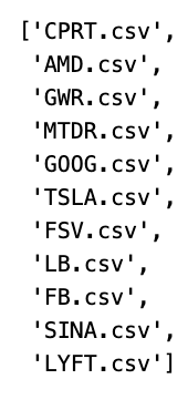
The code generates a list named “stocks” that includes filenames from the current directory, but only those with a “.csv” extension and without the substring “TWTR.” Let’s unpack the workings of this script step-by-step.
First off, the code employs a list comprehension to sift through files in the present directory. Using os.listdir(os.getcwd()), it comprises the iteration through all filenames in the current working directory. For each file name that comes up during this sweep, two checks are performed.
The initial checkpoint is seeing if the file name has “.csv” within it. This ensures that only CSV files are earmarked for further scrutiny. The second condition verifies that the substring ‘TWTR’ is not a part of the file name. Essentially, the file name must be free from this specific text.
When a file name fits both these criteria, it gains a spot in the “stocks” list. So, the code works its magic to filter out unwanted elements, handpicking only those CSV files that don’t mention ‘TWTR’. This selection mechanism proves handy for processing a particular subset of files present in a directory, tailored by name or file type.
In essence, the aim here is to gather strictly those CSV files which sidestep the ‘TWTR’ mention. With this approach, you avoid wrestling with irrelevant files, making subsequent data operations smoother and more efficient. Whether the task involves analytics, data transformation, or visualizations, such filtering steps form the bedrock of a well-organized workflow.
I’ve got this idea to train my model using the stock data I’ve collected, but I’m thinking of keeping Twitter out of the mix. Instead of including Twitter in the training set, I’m planning on setting it aside specifically for testing purposes. By doing this, I hope to see how well my model performs against data it hasn’t seen before, essentially using Twitter as a benchmark to evaluate its accuracy and reliability.
