


Algorithimic Trading of Apple Stock With keras Using LSTM
Algorithimic Trading of Apple Stock With keras Using LSTM
We employ a Long Short-Term Memory (LSTM) recurrent neural network to formulate an effective trading strategy for Apple stock.

This strategy involves using the LSTM model to predict whether to remain in the market on a given day, based on the opening price of each day.
Subsequently, we evaluate the performance of our LSTM-based trading strategy against two other methods: (1) a buy-and-hold strategy, which involves consistently staying in the market, and (2) a moving average strategy, where the decision to buy is made when the current price is at or above the 50-day moving average, and to sell when it is below this threshold.
from __future__ import division
import pandas as pd
import numpy as np
import datetime
import time
import matplotlib.pyplot as plt

import keras
from keras.models import Sequential
from keras.layers import Dense,Dropout,BatchNormalization,Conv1D,Flatten,MaxPooling1D,LSTM
from keras.callbacks import EarlyStopping,ModelCheckpoint,TensorBoard
from keras.wrappers.scikit_learn import KerasRegressor
from keras.models import load_model
from sklearn.preprocessing import MinMaxScaler
In order to analyze and visualize data, this code imports a variety of Python libraries, including pandas, numpy, datetime, time, and matplotlib.pyplot. A number of modules from the Keras library are imported for the purpose of building neural network models. In addition, the code imports modules for training, evaluating, and loading models. Data normalization is completed using Scikit-learns MinMaxScaler.
Part 1: Data Acquisition
Our source for Apple stock data was Yahoo Finance, covering the period from January 6, 2016, to January 5, 2021. Our approach focuses on daily analysis, basing all decisions on the opening price of each day.
The rationale for beginning our analysis 50 days post-January 6, 2016, and concluding it a day prior to January 5, 2021, will be made clear in the forthcoming code section.
To retrieve and process the trading data for Apple stock, we utilized Yahoo Finance in conjunction with the DataReader tool.
# Identify stock data to grab by ticker
ticker = 'AAPL'

start_date=datetime.datetime(2016,1,6)
end_date=datetime.datetime(2021,1,5)
The ticker variable is set to AAPL and the date ranges are defined. Once the data is read from a CSV file, it converts the dates into the correct format. Data is then made more usable by removing the Date column.
Download the source code from the link in comment section.
# For reading stock data from yahoo
from pandas_datareader.data import DataReader

df = DataReader(ticker, 'yahoo', start_date, end_date)

df.drop("Adj Close",axis=1,inplace=True) # May have to adjut columns later
To retrieve stock data from Yahoo, this code imports the pandas_datareader library’s DataReader function. In the next step, it uses this function to create a dataframe with the ticker, start date, and end date specified. Last but not least, it removes the Adj Close column from the dataframe, with the potential to adjust other columns in the future.
For each day, our data set includes three key prices: the day’s closing price, the closing price from the previous day, and the opening price for the next day.
We introduce a feature named *rapp*, which is calculated as the ratio of the previous day’s closing price to the current day’s closing price. This feature is crucial as it represents the daily return or variation in the portfolio’s value.
df['Prev_Close']=df['Close'].shift(1)
df.head()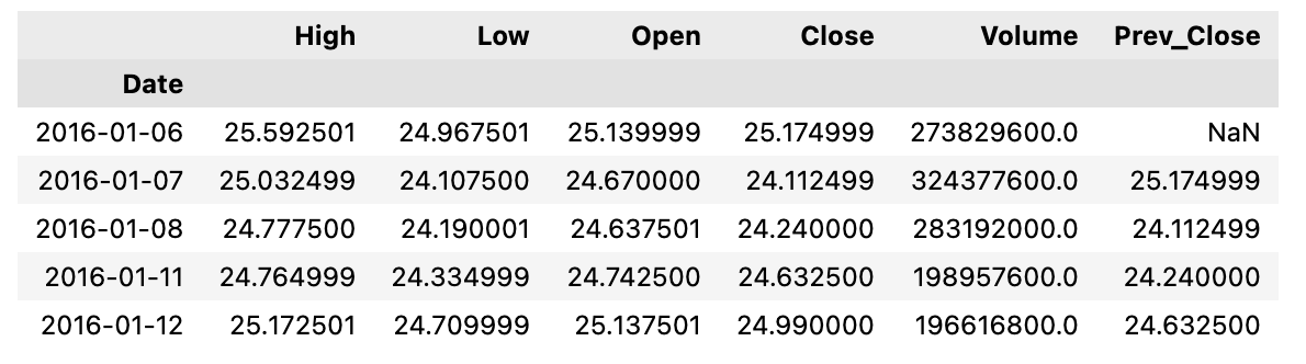
By using this code, we create a column called Prev_Close that contains the previous days’ closing prices in the dataframe called df. Afterwards, the modified dataframe is displayed for the first five rows.
df["rapp"]=df["Close"].divide(df['Close'].shift(1)) # Should be the close of the previous closeDataframe df is created with a new column named rapp. Here, you can see how close the current value is to the previous days value divided by the current value. It assigns each row in the dataframe with its corresponding row in the rapp column as a result of this calculation.
df.head(10)
The following Python code retrieves the first 10 rows of a dataframe.
print(df.head())
print(df.tail())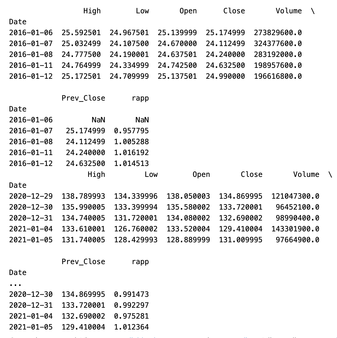
In this Python code, the first and last rows of the provided DataFrame are displayed, containing a summary of what they have to offer.
We are now incorporating two new columns into our data set, which represent the 5-day and 50-day moving averages.
df["mv_avg_short"]= df["Close"].rolling(window=5).mean()
df["mv_avg_long"]= df["Close"].rolling(window=50).mean()
There are two new columns in the dataframe df created by this code: mv_avg_short and mv_avg_long. This column is calculated using the rolling mean function, which takes the Close column as input and calculates the average for a defined window size of 5 and 50. In the original dataframe, these new columns can be used to track short-term and long-term moving averages of Close values.
print(df.loc["2020-12","mv_avg_short"])
print(df.loc["2019-12":"2020-11","Open"])
print(df.loc["2019-12":"2020-11","Open"].mean())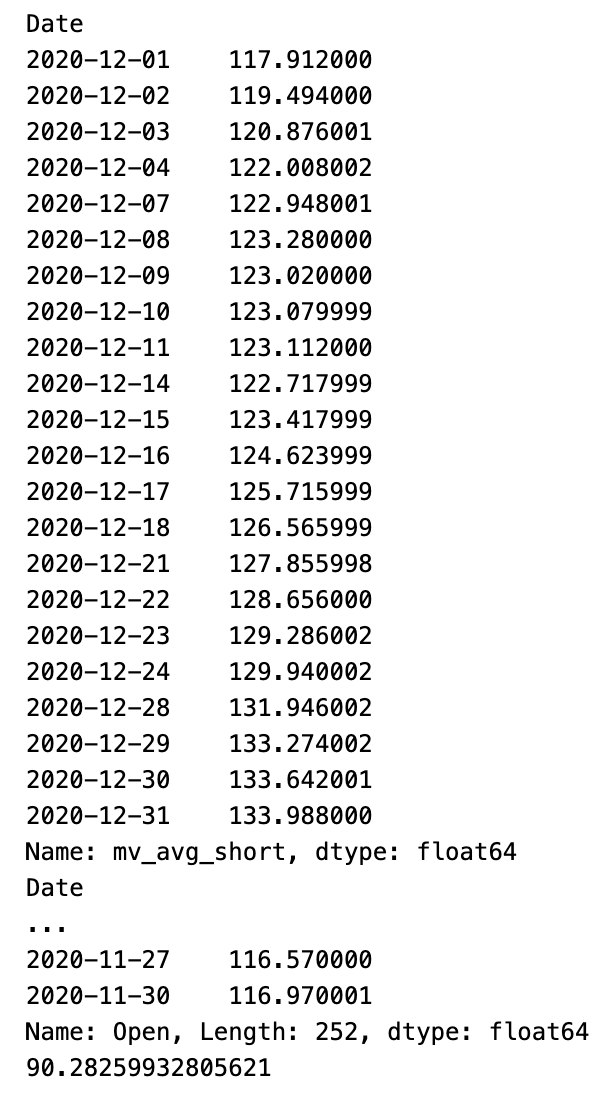
As of 2020–12, the df dataframe contains values for the mv_avg_short column. In the df dataframe, the Open column is printed for the dates between 2019–12 and 2020–11. As a final step, it prints an average of the dates between 2019–12 and 2020–11 in the Open column.
We are excluding the initial 50 days from our analysis because they lack the data necessary to calculate the 50-day moving average.
df=df.iloc[50:,:] # WARNING: DO IT JUST ONE TIME!
print(df.index)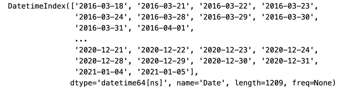
A variable named df is created by selecting all rows from index 50 to the end of the dataframe. This modified dataframe’s index is also printed. As suggested by the warning, this operation should be done only once.
Finally, we can divide *df* in train and test set
mtest=300
train=df.iloc[:-mtest,:]
test=df.iloc[-mtest:,:]
As a result of this code, three dataframes are created: a train with all rows in the original dataframe and a test with the last 300 rows, and a df with all rows.
print(len(train))
print(len(test))
print(len(df))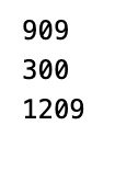
A length will be printed for the variables train, test, and df in this code.
Gross Yield Calculation Functions
It’s important to note that calculating the gross yield is straightforward when using the rapp feature. The subsequent function demonstrates this process: it employs the vector ‘v’ to determine the specific days we will remain active in the market.
# This function returns the total percentage gross yield and the annual percentage gross yield

def yield_gross(df,v):
    prod=(v*df["rapp"]+1-v).prod()
    n_years=len(v)/252
    return (prod-1)*100,((prod**(1/n_years))-1)*100
Based on the input data and parameters, this function calculates the gross yield percentage and the annual yield percentage. The calculation of gross yield is based on the input data frame and a specified parameter v, and the output is converted to percentages. Afterwards, the function returns a pair containing the total and annual gross yields.
Define The LSTM Model
We aim to deploy a Long Short-Term Memory (LSTM) neural network to determine our daily market involvement during the test period, based on each day’s opening stock price.
This necessitates reshaping our data to fit the specific format required by the LSTM, which involves the use of “windows.” At each step, our objective is to predict the day’s closing price. This prediction will enable us to derive the vector ‘v,’ which will be used to select the days we will stay in the market.
def create_window(data, window_size = 1):
    data_s = data.copy()
    for i in range(window_size):
        data = pd.concat([data, data_s.shift(-(i + 1))], axis = 1)

    data.dropna(axis=0, inplace=True)
    return(data)
A dataset is provided in this code, and offset copies are created according to the specified window size. Hence, the original data becomes shifted in a new dataset. Incomplete rows are then dropped from the new dataset before it is finally returned.
scaler=MinMaxScaler(feature_range=(0,1))
dg=pd.DataFrame(scaler.fit_transform(df[["High","Low","Open","Close","Volume",\
                                          "mv_avg_short","mv_avg_long"]].values))
dg0=dg[[0,1,2,3,4,5]]


window=4
dfw=create_window(dg0,window)

X_dfw=np.reshape(dfw.values,(dfw.shape[0],window+1,6))

y_dfw=np.array(dg[6][window:]) # The Fix
It simplifies a dataset by calculating the minimum and maximum values, and then converting them to 0 or 1. By taking in a DataFrame that contains high, low, open, close, volume, and moving average data, it creates a DataFrame that has values scaled between 0 and 1. Next, it builds a sliding window of size 4 for predicting future values and then converts the data into numpy arrays.
X_trainw=X_dfw[:-mtest-1,:,:]
X_testw=X_dfw[-mtest-1:,:,:]
y_trainw=y_dfw[:-mtest-1]
y_testw=y_dfw[-mtest-1:]
A dataset X_dfw and y_dfw is split based on mtest into two parts to create two train and test sets. Initially, a machine learning model is trained and then tested.
def model_lstm(window,features):

    model=Sequential()
#     model.add(LSTM(600, input_shape = (window,features), return_sequences=True))
#     model.add(Dropout(0.5))
    model.add(LSTM(300, input_shape = (window,features), return_sequences=True))
    model.add(Dropout(0.5))
    model.add(LSTM(200, input_shape=(window,features), return_sequences=False))
    model.add(Dropout(0.5))
    model.add(Dense(100,kernel_initializer='uniform',activation='relu'))
    model.add(Dense(1,kernel_initializer='uniform',activation='relu'))
    model.compile(loss='mse',optimizer='adam')


    return model
In this code, a recurrent neural network RNN has been used to process sequential data using the Long Short-Term Memory architecture. A window of data with features is taken as input shape, and three LSTM layers are used along with three dropout layers. After adding two dense layers and setting the loss function and optimizer, the model is compiled before returning.
model=model_lstm(window+1,6)
history=model.fit(X_trainw,y_trainw,epochs=100, batch_size=30, validation_data=(X_testw, y_testw), \
                  verbose=1, callbacks=[],shuffle=False) # Batch size should be no more than the square root of the # of training rows

plt.plot(history.history['loss'])
plt.plot(history.history['val_loss'])
plt.title('model loss')
plt.ylabel('loss')
plt.xlabel('epoch')
plt.legend(['train', 'test'], loc='upper right')
plt.show()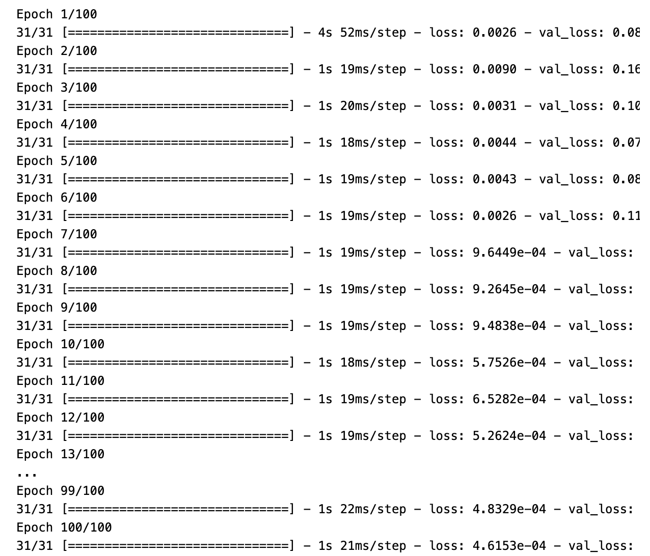
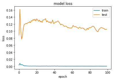
An LSTM model is trained with a specified window size and six features using this code. Data is divided into training and validation sets in order to train the model over 100 epochs with a batch size of 30. A graph is displayed to show both training and validation sets’ loss values.