

Algorithmic Trading and Financial Backtesting with Zipline and Pyfolio-Chapter 3
Exploring Mean Reversion, Risk Metrics, and Performance Visualization in Algorithmic Trading Strategies

Algorithmic trading has revolutionized the way financial strategies are developed and executed. This article explores the use of Zipline, a powerful Python library for backtesting and analyzing trading algorithms, alongside Pyfolio, a tool for performance and risk analysis. By leveraging these libraries, we can design and test a mean reversion strategy, analyze key performance metrics, and visualize crucial aspects such as returns, volatility, drawdowns, and portfolio risk. Through this process, the goal is to gain insights into the strategy’s effectiveness, optimize decision-making, and better understand financial market behavior.
import sys
from pathlib import Path
import pandas as pd
from pytz import UTC
from zipline import run_algorithm
from zipline.api import (attach_pipeline, date_rules, time_rules, order_target_percent,
                         pipeline_output, record, schedule_function, get_open_orders, calendars,
                         set_commission, set_slippage)
from zipline.finance import commission, slippage
from zipline.pipeline import Pipeline, CustomFactor
from zipline.pipeline.factors import Returns, AverageDollarVolume
import logbook
import matplotlib.pyplot as plt
import seaborn

from pyfolio.utils import extract_rets_pos_txn_from_zipline
A zipline backtesting library is used to set up an environment for running an algorithmic trading strategy. In order to start, it imports essential modules, like sys and pathlib for system operations, pandas for finance, and pytz for consistent timestamp handling in UTC. Additionally, Zipline is used for creating and managing trading algorithms, so it imports those components too. Among the key functions are run_algorithm, attach_pipeline, pipeline_output, order_target_percent, track performance over time, schedule_function, and get_open_orders. They’re all useful for executing a trading strategy within a given date range, attach_pipeline, and pipeline_output.
Moreover, the code imports commission and slippage settings from Zipline’s finance module to simulate realistic trading conditions, where commissions represent fees during trading and slippages account for price discrepancies. By using CustomFactor, investment strategies can be customized. Additionally, logbook is imported for activity logging, seaborn for data visualization, and utilities from Pyfolio for analysis after execution. Basically, this code lays the groundwork for building, executing, and analyzing an algorithmic trading strategy.
sns.set_style('darkgrid')Set_style specifies the visual appearance of your plots. This line uses the Seaborn library, a popular Python data visualization library. Seaborn’s darkgrid argument creates a style with a dark background and grid overlay that enhances plot readability and lets you interpret the data more easily. Dark backgrounds make plot colors easier to see. It gives your visualizations a polished, professional look by establishing a style before you create them.
# setup stdout logging
zipline_logging = logbook.NestedSetup([
    logbook.NullHandler(level=logbook.DEBUG),
    logbook.StreamHandler(sys.stdout, level=logbook.INFO),
    logbook.StreamHandler(sys.stderr, level=logbook.ERROR),
])
zipline_logging.push_application()
Using the Logbook library, this code snippet configures multiple logging handlers. The NullHandler is at the DEBUG level, so it ignores log messages and doesn’t warn about missing handlers. Then two StreamHandler instances are created: one that sends INFO messages to standard output, and the other that sends ERROR messages to standard error for critical problems. Then you call push_application to activate this logging configuration, so you can manage messages based on severity.
# Settings
MONTH = 21
YEAR = 12 * MONTH
N_LONGS = 200
N_SHORTS = 0
VOL_SCREEN = 1000
For later use, I’ve set MONTH to 21, which indicates a time period in months. YEAR is calculated by multiplying MONTH by 12, which results in 252 months. In a trading strategy, N_LONGS indicates how many long positions there are, whereas N_SHORTS indicates that there are no short positions, which indicates that buying is the priority. VOLSCREEN is set to 1000, which ensures only assets with trading volumes above this threshold are considered. These constants set the parameters for the next steps.
start = pd.Timestamp('2010-01-01', tz=UTC)
end = pd.Timestamp('2018-01-01', tz=UTC)
capital_base = 1e7
Two variables are initialized using Panda’s Timestamp and a capital base value. Start and end are defined as timestamps to indicate the beginning and end of a time period. Using pd.Timestamp, we give a string date and set the timezone to UTC with start and end set to January 1, 2010. In financial analysis or modeling, capital_base can serve as the initial amount of capital. Timeframes and starting points are set here.
class MeanReversion(CustomFactor):
    """Compute ratio of latest monthly return to 12m average,
       normalized by std dev of monthly returns"""
    inputs = [Returns(window_length=MONTH)]
    window_length = YEAR

    def compute(self, today, assets, out, monthly_returns):
        df = pd.DataFrame(monthly_returns)
        out[:] = df.iloc[-1].sub(df.mean()).div(df.std())
MeanReversion evaluates mean reversion by comparing the latest month’s return with the average month’s return over the past year, normalizing the difference by the standard deviation. The inputs attribute specifies that the analysis focuses on monthly returns, while the Returns function fetches data from the last month. By setting the window length to one year, all calculations use yearly data.
It takes parameters like today as the current date, assets as the assets to be analyzed, out as the storage location for the results, and monthly_returns as the last year’s data. You can manipulate the monthly returns in pandas DataFrames. You just subtract the mean of previous monthly returns, divide by the standard deviation, and take the most recent monthly return. The normalization lets you see how far the latest return deviates from the average. Based on the previous year’s performance, a score is given to the output array, indicating how much the latest return is an outlier.
def compute_factors():
    """Create factor pipeline incl. mean reversion,
        filtered by 30d Dollar Volume; capture factor ranks"""
    mean_reversion = MeanReversion()
    dollar_volume = AverageDollarVolume(window_length=30)
    return Pipeline(columns={'longs'  : mean_reversion.bottom(N_LONGS),
                             'shorts' : mean_reversion.top(N_SHORTS),
                             'ranking': mean_reversion.rank(ascending=False)},
                    screen=dollar_volume.top(VOL_SCREEN))
A pipeline of financial factors identifies trading opportunities using mean reversion. Using a MeanReversion object, it evaluates stocks based on price movements and the likelihood that they’ll revert to average prices. To ensure that only stocks with significant liquidity are considered for analysis, an AverageDollarVolume instance is created with a 30-day window.
Three main columns make up the pipeline. The longs column selects poorly performing stocks based on mean reversion criteria, defined by a parameter for how many long positions there are. Top-performing stocks are identified in the shorts column by using the same criteria, with a parameter for how many shorts they have. Stocks get ranked descending by mean reversion logic in the ranking column.
As part of the pipeline, only stocks that meet the dollar volume criteria are included, which means they’ve been trading well lately and are more likely to be successful. By using a mean reversion analysis, this function identifies long and short positions, while ensuring sufficient liquidity with a dollar volume filter.
def before_trading_start(context, data):
    """Run factor pipeline"""
    context.factor_data = pipeline_output('factor_pipeline')
    record(factor_data=context.factor_data.ranking)
    assets = context.factor_data.index
    record(prices=data.current(assets, 'price'))
At the start of a trading period, the before_trading_start function runs a factor pipeline used to evaluate stocks based on certain criteria in quantitative finance. Upon calling this function, it retrieves the output of the factor pipeline with the pipeline_output function and stores it in context.factor_data, which contains information about a bunch of assets. In order to analyze performance over time, the function records rankings using the record function. The assets variable provides a list of relevant assets based on the indexes in context.factor_data. It also uses the data.current method to get and record the current prices of these assets, which is important to understand the market context. It’s a crucial function for preparing before trading activities, allowing for data-driven decisions based on market conditions.
def rebalance(context, data):
    """Compute long, short and obsolete holdings; place trade orders"""
    factor_data = context.factor_data
    assets = factor_data.index

    longs = assets[factor_data.longs]
    shorts = assets[factor_data.shorts]
    divest = context.portfolio.positions.keys() - longs.union(shorts)

    exec_trades(data, assets=divest, target_percent=0)
    exec_trades(data, assets=longs, target_percent=1 / N_LONGS if N_LONGS else 0)
    exec_trades(data, assets=shorts, target_percent=-1 / N_SHORTS if N_SHORTS else 0)
In the rebalance function, outdated holdings get liquidated, and long and short positions are rebalanced based on the factors you provide. Factor data is the first step, which contains information on a variety of assets and trading signals. Assets are the ones in this data that are included in the assets variable.
The function defines three groups of assets: longs, which are for long positions; shorts, which are for short positions; and divest, which is assets currently in the portfolio that aren’t long or short, calculated by subtracting the union of long and short assets.
When divest assets are called, it calls exec_trades with a target percent of 0. Then it liquidates the positions. Depending on how many longs there are, it distributes investment equally among them, or it sets 0% if there are no longs at all. Using the number of short positions, it makes sure money is allocated evenly in the negative direction.
In this way, the portfolio is continuously optimized based on the latest trading signals and positions are managed effectively.
def exec_trades(data, assets, target_percent):
    """Place orders for assets using target portfolio percentage"""
    for asset in assets:
        if data.can_trade(asset) and not get_open_orders(asset):
            order_target_percent(asset, target_percent)
In the exec_trades function, you give three parameters: data, assets, and target_percent. It places orders for certain assets in accordance with a target percentage. This function checks if trading is allowed on each asset and if there aren’t any open orders for that asset in the assets list. As soon as both conditions are met, it calls order_target_percent, which sets the asset’s target allocation. The approach ensures efficient trade management by placing orders only when they’re allowed and when there aren’t any pending orders.
def initialize(context):
    """Setup: register pipeline, schedule rebalancing,
        and set trading params"""
    attach_pipeline(compute_factors(), 'factor_pipeline')
    schedule_function(rebalance,
                      date_rules.week_start(),
                      time_rules.market_open(),
                      calendar=calendars.US_EQUITIES)

    set_commission(us_equities=commission.PerShare(cost=0.00075, min_trade_cost=.01))
    set_slippage(us_equities=slippage.VolumeShareSlippage(volume_limit=0.0025, price_impact=0.01))
The initialize function sets up the environment for a trading algorithm. It configures the necessary components so it will work. The pipeline is registered using attach_pipeline, which collects data and calculates factors influencing trading decisions. A rebalance function adjusts portfolio holdings at the beginning of every week when the market opens, making sure trades are executed on time.
Furthermore, the commission is set with set_commission, with a minimum price of $0.01 and a cost per share of $0.00075. That way, even if there’s not much share volume, there’s a minimum fee. By setting slippage to 0.0025 and assuming 1% price impact per trade, the trading strategy collects data effectively, manages holdings, and operates within defined costs and risks.
backtest = run_algorithm(start=start,
                         end=end,
                         initialize=initialize,
                         before_trading_start=before_trading_start,
                         capital_base=capital_base)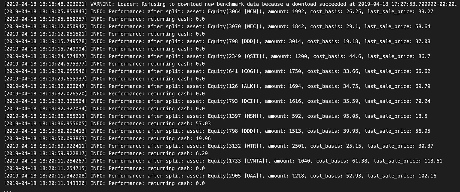
A backtest is performed with the run_algorithm function from Zipline, a library that you need to trade algorithmically. Start and end are parameters for backtesting, initialize is for setting up the trading algorithm, before_trading_start is for making pre-trade adjustments, and capital_base is for specifying the strategy’s initial capital.
In the output log, you can see the backtest execution, starting with a warning about benchmark data not being available, but confirming that data had already been downloaded. Performance metrics are shown in the log entries marked INFO during the backtest. They show the amount, cost basis, and cash balance of various assets.
For example, Equity(3064 [WCN]) and Equity(3070 [WEC]) performance is documented along with their amounts and cost bases. During trading, the cash balance changes, reflecting trade results. Also, entries tell you how stocks performed after stock splits, which is important to figure out how they impacted portfolio value.
During the backtest, the log shows how the trading strategy affects performance at regular intervals. As a result of the final entries, the backtest spans the year 2013, so users can assess the effectiveness of their trading strategy, assess risks, and make informed adjustments.
returns, positions, transactions = extract_rets_pos_txn_from_zipline(backtest)This line of code calls the function extract_rets_pos_txn_from_zipline with the backtest variable as an argument. It gets specific info about a backtest using Zipline, a Python algorithmic trading library. There are three data points in it: returns, positions, and transactions. The returns contain the strategy performance, such as profit or loss. Positions show the assets you held during the backtest. The transactions detail the executed trades throughout the backtest, including the buy and sell activities. Tuple unpacking makes assigning the outputs easy.
with pd.HDFStore('backtests.h5') as store:
    store.put('backtest', backtest)
    store.put('returns', returns)
    store.put('positions', positions)
    store.put('transactions', transactions)
A data component from a backtesting process is stored in HDF5 files using the pandas library. HDFStore context manager makes sure the data is safe and secure. In this context, the put method saves datasets such as backtests, returns, positions, and transactions, which are important for backtesting results and make data storage and retrieval easier.
There could be issues with serializing certain object types in HDF5, since the data may contain elements that can’t be mapped to C-types. The warnings about performance issues emphasize the need to make sure the stored data is HDF5 compatible, especially for complex data structures and custom objects.
fig, axes= plt.subplots(nrows=2, figsize=(14,6))
returns.add(1).cumprod().sub(1).plot(ax=axes[0], title='Cumulative Returns')
transactions.groupby(transactions.dt.dt.day).txn_dollars.sum().cumsum().plot(ax=axes[1], title='Cumulative Transactions')
fig.tight_layout();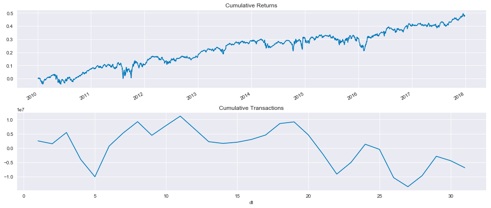
This code snippet generates a figure with two subplots that visualize financial data from a mean reversion backtest using Zipline. The first subplot shows cumulative returns over time, while the second subplot shows cumulative transaction values over time.
Adding one to the returns and computing the cumulative product track the growth of an investment starting with one in the first subplot. It usually trends upward, so the investment strategy is profitable, but it fluctuates from time to time.
It shows the total transaction volume over time by summing up the daily transaction dollars and calculating the cumulative amount. Due to the fluctuating nature of trading activity, this plot is more variable than the cumulative returns.
The layout facilitates comparisons between cumulative returns and transaction activity. Together, these visualizations offer insight into the performance of the trading strategy and transaction dynamics.
positions.info()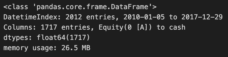
Positions.info() is in Pandas, which lets you analyze and manipulate data in Python. This is a summary of the DataFrame, which in this case tracks position in a backtesting project using the Zipline framework for mean reversion strategies. Over the course of a substantial time period, the DataFrame contains 1717 entries, indicating a chronological organization that makes it easy to analyze. Equity and cash indicate that it represents the value of assets and investments over time, emphasizing cash. With float64 data types, the values are floating-point numbers, perfect for financial data with decimals. It’s pretty modest in terms of memory usage given how many entries it has, which is good to know about data handling efficiency. Positions.info() provides insight into the DataFrame’s structure and content, allowing users to gauge whether the data is ready for further analysis or modeling.
transactions.describe()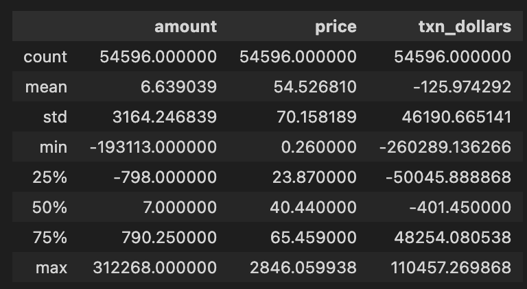
In a mean reversion backtest project, transactions.describe() generates descriptive statistics for a DataFrame called transactions. There are 54,596 entries in each column, indicating a huge dataset, with three key columns: amount, price, and txn_dollars. Approximately 6.64 transactions are made, with an average price per unit of 54.53, and an average dollar value of -125.97, which suggests the dataset is mostly sales or losses.
As you can see from the standard deviation values, the amount has a high standard deviation, 3164.43, indicating that it fluctuates a lot. -19,313 is the minimum transaction amount, indicating a lot of sell-offs or negative transactions, whereas 312,268 is the maximum, indicating a lot of transactions. In the quartiles, there’s a 25th percentile of amount at -798, meaning 25% of transactions are below that value, a median of 7 indicates half of transactions are below that amount, and a 75th percentile at 790.25, which means most transactions aren’t that big.
Using this analysis, we can get a clear overview of the transaction data, revealing patterns and outliers that help us understand the performance and behavior of our trading strategy.
from pathlib import Path
import warnings
import re
import numpy as np
import pandas as pd
import seaborn as sns
import matplotlib.pyplot as plt
Path from pathlib simplifies file path manipulation. This code snippet imports Python libraries and modules for data manipulation, visualization, and file handling. With the warnings module, you can control how warning messages show, so you don’t crash. With the re module, strings can be searched and patterns can be matched with regular expressions. With Numpy, you can run arrays and use mathematical functions. Pandas is perfect for analyzing structured data, and DataFrames make it easy to manipulate and clean. A popular library for creating static, animated, and interactive data visualizations is Matplotlib.pyplot, built on Matplotlib. Seaborn makes it easy to create attractive statistical visualizations using Matplotlib.pyplot. These libraries provide a robust foundation for handling data, performing analyses, and generating visual insights. Path handles data files, Pandas and Numpy handle data manipulation, and Seaborn and Matplotlib visualize the results.
from pyfolio.utils import extract_rets_pos_txn_from_zipline
from pyfolio.plotting import (plot_perf_stats,
                              show_perf_stats,
                              plot_rolling_beta,
                              plot_rolling_fama_french,
                              plot_rolling_returns,
                              plot_rolling_sharpe,
                              plot_rolling_volatility,
                              plot_drawdown_periods,
                              plot_drawdown_underwater)

from pyfolio.timeseries import perf_stats, extract_interesting_date_ranges
# from pyfolio.tears import create_returns_tear_sheet
For financial portfolio performance analysis, this code imports Pyfolio functions. For performance analysis of trading strategies, extract_rets_pos_txn_from_zipline from pyfolio.utils extracts returns, positions, and transactions from Zipline backtest results.
Several plotting functions are then imported from pyfolio.plotting to visualize portfolio performance, including plot_perf_stats to summarize overall performance statistics, show_perf_stats to output statistics directly, plot_rolling_beta to measure portfolio volatility relative to a benchmark, plot_rolling_fama_french to visualize performance concerning Fama-French factors, plot_rolling_returns to display rolling returns, plot_rolling_sharpe to assess risk-adjusted returns, plot_rolling_volatility to illustrate changes in portfolio volatility, plot_drawdown_periods to highlight periods of drawdowns, and plot_drawdown_underwater to visualize how far the portfolio is underwater during drawdowns.
From pyfolio.timeseries, perf_stats calculates key performance metrics, while extract_interesting_date_ranges identifies specific dates for deeper analysis of performance extremes or drawbacks. Similarly, create_returns_tear_sheet is commented out, suggesting its potential usefulness for generating detailed performance metrics reports for a set of returns, although it is not currently required.
%matplotlib inline
plt.style.use('fivethirtyeight')
warnings.filterwarnings('ignore')
This snippet configures the Jupyter Notebook environment for data visualization with Matplotlib. The command %matplotlib inline enables plots to appear directly in the notebook, allowing for easy viewing of visual output. The command plt.style.use(‘fivethirtyeight’) applies a style to the plots that resembles the FiveThirtyEight website, enhancing the visual appeal with a clean and modern look. Additionally, warnings.filterwarnings(‘ignore’) suppresses warning messages that may clutter the output, providing a cleaner workspace during exploratory data analysis or prototyping. These commands facilitate the visualization process and enhance aesthetics in data analysis.
with pd.HDFStore('../01_trading_zipline/backtests.h5') as store:
    backtest = store['backtest']
backtest.info()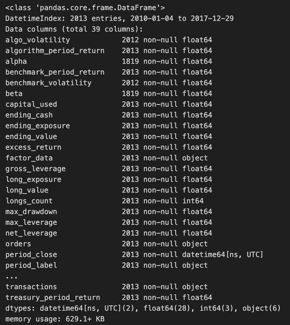
The code snippet uses the pandas library to access data from an HDF5 file, specifically a dataset named backtest. It employs a with statement to open and close the HDF5 file efficiently, using the pd.HDFStore function to manage the file located at ../01_trading_zipline/backtests.h5. Within this context, the backtest dataset is loaded into the backtest variable.
The output of the backtest.info() method summarizes the DataFrame’s structure, indicating a DatetimeIndex from January 4, 2010, to December 29, 2017, with 2013 entries. It includes 30 columns representing various metrics related to backtesting results, such as algorithm_period_return, alpha, benchmark_period_return, and excess_return, which are essential for assessing trading strategy performance.
The column data types vary, with most being float64, indicating numerical values, while others are int64 or object, potentially containing categorical data or timestamps. The presence of non-null entries in most columns indicates a complete dataset, which is crucial for accurate analysis. The output also provides the DataFrame’s memory usage, which is 629.1 KB, essential for understanding the dataset’s complexity and the computational resources needed for further analysis.
returns, positions, transactions = extract_rets_pos_txn_from_zipline(backtest)This line of code calls the function extract_rets_pos_txn_from_zipline and passes the variable backtest to it. The function is expected to return three values: returns, positions, and transactions. Returns contains the performance data associated with the backtested trading strategy, positions provides information about the shares or contracts held at different times during the backtest, and transactions details the trades executed, including buys and sells. This function extracts essential metrics and data from the backtest, enabling effective assessment and analysis of the results.
returns.head().append(returns.tail())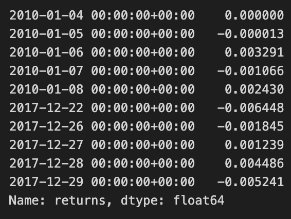
The code snippet returns.head().append(returns.tail()) provides a concise overview of a DataFrame with financial return data. The head() method retrieves the initial rows, while tail() retrieves the final rows. By appending these two sets, the code combines the earliest and latest entries, offering a snapshot of returns over time.
The output displays return values indexed by date from January 4, 2010, to December 29, 2017. The initial rows reflect returns for early January 2010, with values ranging from 0.000000 to -0.003291. The last entries from late 2017 present a mix of positive and negative returns, with the final value at -0.005241. This output illustrates the fluctuations in returns, providing insights into the asset’s performance at both the start and end of the observed period.
This method effectively helps analysts quickly assess investment performance trends, showing how returns have evolved from the beginning to the end of the dataset.
positions.columns = [c.symbol for c in positions.columns[:-1]] + ['cash']
positions.index = positions.index.normalize()
positions.info()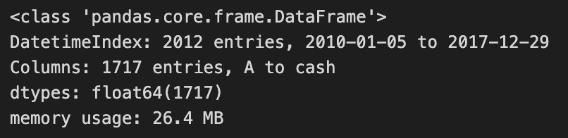
The code modifies a DataFrame named positions, which contains financial data for a trading strategy. It first updates the column names by replacing the last column with the term ‘cash’, indicating it represents cash holdings, a common practice in managing financial data. Then, it normalizes the DataFrame’s index by removing the time component from any datetime entries, allowing for easier date comparison.
The code outputs a summary of the modified DataFrame, which is of type pandas.core.frame.DataFrame, containing 2,012 entries from January 5, 2010, to December 29, 2017. It includes 1,717 columns, featuring asset symbols and the new ‘cash’ column. All entries are of data type float64, suggesting they represent numerical monetary values. The DataFrame’s memory usage is 26.4 MB, indicating its resource consumption. This code effectively prepares the DataFrame for analysis or visualization by ensuring proper formatting of column names and the index.
transactions.symbol = transactions.symbol.apply(lambda x: x.symbol)This line of code uses the apply function on the symbol column of the transactions DataFrame to transform each entry by applying a lambda function. The lambda function takes one argument and extracts the symbol attribute from each object in the symbol column. Consequently, after executing this line, the symbol column will only contain the values of the symbol attribute for each original entry. This transformation is useful when the original entries are objects, allowing you to retain just their symbol values as strings or another type.
transactions.head().append(transactions.tail())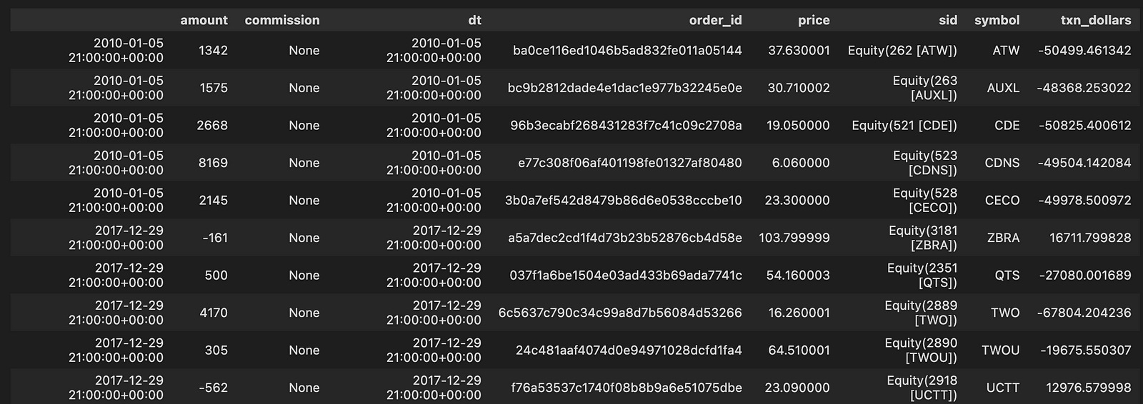
The code snippet transactions.head().append(transactions.tail()) combines the first five and last five rows of a DataFrame named transactions. This operation allows for a quick examination of the beginning and end of the dataset, which can help identify trends or anomalies. The resulting DataFrame includes columns such as amount, commission, dt, order_id, price, sid, symbol, and txn_dollars, with data from January 5, 2010, to December 29, 2017. Each row represents a transaction, detailing the transaction amount, commission, date and time, order ID, price, and security symbol.
For example, the first transaction from January 5, 2010, shows an amount of 1342 and a price of 37.630001, while the last transaction on December 29, 2017, has an amount of -562 with a price of 23.090000. This combination of the head and tail allows users to view both the initial and final transactions, providing a snapshot of the data’s range and insights into the evolution of transactions over time. The output illustrates the structure and content of the transactions DataFrame, facilitating analysis of the financial data across the timeline.
HDF_PATH = Path('..', '..', 'data', 'assets.h5')This line of code defines a variable named HDF_PATH that stores the path to a file called assets.h5. The Path function is from the pathlib module, allowing for easy manipulation of file paths. By using Path(‘..’, ‘..’, ‘data’, ‘assets.h5’), it creates a relative path that navigates up two directories and into the data folder containing the assets.h5 file. This method enhances code portability by avoiding hard-coded full paths that may differ in various environments. Therefore, HDF_PATH specifies the location of the assets.h5 file in a flexible and clean manner.
assets = positions.columns[:-1]
with pd.HDFStore(HDF_PATH) as store:
    df = store.get('us_equities/stocks')['sector'].dropna()
    df = df[~df.index.duplicated()]
sector_map = df.reindex(assets).fillna('Unknown').to_dict()
This code manages sector data for a set of assets stored in an HDF5 file. It starts by identifying the asset columns in the positions DataFrame, excluding the last column. It then opens the HDF5 store at HDF_PATH with a context manager to ensure proper closure after use. Within this context, it retrieves the ‘sector’ DataFrame from the us_equities/stocks key and removes any entries with missing values in the sector column to clean the data.
Next, it eliminates duplicate indices in the DataFrame by filtering for unique index records. The DataFrame is reindexed to match the asset list, and any asset lacking a corresponding sector entry is assigned a NaN, which is then replaced with ‘Unknown’. Finally, the processed DataFrame is converted to a dictionary that maps each asset to its respective sector, facilitating quick lookups and defaulting to ‘Unknown’ for assets that are not found.
with pd.HDFStore(HDF_PATH) as store:
    benchmark_rets = store['sp500/prices'].close.pct_change()
benchmark_rets.name = 'S&P500'
benchmark_rets = benchmark_rets.tz_localize('UTC').filter(returns.index)
benchmark_rets.tail()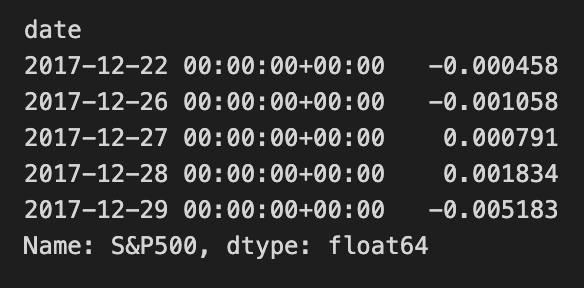
The code snippet uses the pandas library to process financial data stored in HDF5 format. It accesses the HDF5 store at HDF_PATH to retrieve the closing prices of the S&P 500 index and applies the pct_change method to compute the percentage change between consecutive closing prices, converting the price data into returns, which are vital for financial analysis.
After calculating the returns, the code labels the resulting Series as ‘S&P500’ for easier identification. It uses the tz_localize(‘UTC’) method to standardize the timestamps to UTC. The filter(returns.index) method aligns the benchmark returns with another Series called returns, ensuring that only the dates present in the returns index remain in the benchmark_rets Series.
The output shows the last few entries of the benchmark_rets Series, which captures the date and corresponding daily percentage returns for the S&P 500, indicating both positive and negative fluctuations over the specified period. This output also confirms that the return values are of float64 type, suitable for numerical calculations in financial analysis. This process is crucial for further analysis, such as risk assessment or performance comparison, in transitioning the project from Zipline to Pyfolio.
perf_stats(returns=returns, factor_returns=benchmark_rets, positions=positions, transactions=transactions)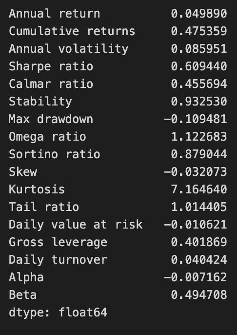
The function perf_stats evaluates the performance of a trading strategy by analyzing various financial metrics from the provided returns, benchmark returns, positions, and transactions. The output includes key performance indicators that assess the strategy’s effectiveness and risk profile.
The annual return is approximately 0.0499, indicating the average yearly profit, while cumulative returns are about 0.4754, reflecting total returns over the analyzed period. Annual volatility is around 0.0859, measuring return variation and associated risk. The Sharpe ratio, approximately 0.6094, indicates a reasonable return per unit of risk.
The Calmar ratio is about 0.4557, comparing annual returns to a maximum drawdown of -0.1095, which shows the largest decline in investment value and highlights significant loss potential. Stability, valued at 0.9323, suggests consistent performance.
Other metrics include an Omega ratio of 1.1227, indicating the likelihood of higher returns compared to losses, and a Sortino ratio of approximately 0.8790, focusing on downside risk. The skew at -0.0320 indicates a slight tendency towards negative returns, while kurtosis at 7.1644 suggests a higher likelihood of extreme outcomes.
