

Algorithmic Trading Ch-1: Market & Fundamental Data
Building and testing trading strategies requires understanding and using market and fundamental data.

This is a comprehensive series consisting of 33 chapters focused on algorithmic trading. Each chapter will delve deeply into coding aspects, beginning with fundamental concepts and progressively advancing to more complex topics. Regular articles will continue to be published, but this series serves as a dedicated course for my audience interested in algorithmic trading.
Download the source code, at the end!
This chapter introduces those concepts. Backtesting and analysis are highly dependent on understanding orders, trading infrastructure, and data sources. Market microstructure influences market data, and we’ll demonstrate how to manipulate both trading and financial statement data with Python.
Our discussion begins with the placement and execution of orders in financial markets that generate market data. Market microstructure shapes the data used by algorithmic traders to derive insights and trading signals in this chapter. Various methods will be presented for reconstructing order books from tick data, summarizing this data, and accessing market data through different interfaces.
Our next step is to examine fundamental data, including economic factors that influence security values. Data is more readily available in the U.S. market, where this chapter focuses on equity fundamentals. Using financial statements filed with the SEC, using XBRL for automated data processing, and creating fundamental metrics like P/E, we will cover it all.
Last but not least, we will compare the performance and suitability of storing large datasets in Python using CSV, HDF5, and Parquet formats.
Building and testing algorithmic trading strategies requires a thorough understanding of market and fundamental data.
Market Data: Order Book and FIX Protocol
In order to capture every transaction, the order book continuously updates in real-time throughout the trading day. A real-time service from exchanges provides the complete picture of trading activity, including buy and sell orders. Historical data is often free of charge on some exchanges.
Many messages about trade orders are sent by market participants to convey the order book’s data. Market data and securities transactions are typically communicated using the Financial Information eXchange (FIX) protocol. In the back-office sector, FIX serves as the primary messaging standard for exchanges, banks, brokers, and other financial entities during trade execution. Broker-dealers and institutional clients previously communicated via phone exchanges before FIX was introduced in 1992 by Fidelity Investments and Salomon Brothers.
In addition to equity markets, FIX protocol spread to foreign exchange, fixed income, derivatives, and even post-trade processes to support straight-through processing. Exchanges now provide real-time access to FIX messages, which algorithmic traders use to monitor market activity. These messages can be analyzed to detect market participants’ actions and predict their future moves.
Exchanges also offer native data feed protocols. The Nasdaq, for example, offers TotalView ITCH, which enables subscribers to track orders for equity instruments from initial placement to execution and cancellation. A particular security or financial instrument’s order book can be rebuilt using this capability.
In addition to revealing market depth, the order book lists the number of bids and offers throughout the day. In order to assess liquidity and understand how large market orders will impact prices, this depth is crucial. Furthermore, the ITCH protocol includes information such as system events, stock characteristics, limit order placements and modifications, trade executions, and even the net order imbalance before markets open or close. Making informed trading decisions requires these insights.
import gzip
import shutil
from pathlib import Path
from urllib.request import urlretrieve
from urllib.parse import urljoin
from clint.textui import progress
from datetime import datetime
import pandas as pd
import numpy as np
import matplotlib.pyplot as plt
from matplotlib.ticker import FuncFormatter
from struct import unpack
from collections import namedtuple, Counter
from datetime import timedelta
from time import time
Several modules are imported for this code snippet. Work with compressed files and perform high-level file operations with gzip and shutil. Filesystem paths can be manipulated object-oriented with pathlib. Files are downloaded and URLs are constructed using urlretrieve and urljoin. Clint.textui provides progress bars, while datetime and timedelta manage dates and durations. Large datasets require Pandas and Numpy for data analysis and mathematical operations. With FuncFormatter, you can customize tick labels on plots with Matplotlib.pyplot. Using structures, you can manipulate binary data using C, and namedtuples create lightweight objects. Time is included for measuring elapsed time when counting hashable objects from collections. This set of imports indicates the code will download, process, analyze, and visualize large datasets.
By parsing binary ITCH data samples, users can reconstruct executed trades and order books for specific ticks. It requires significant time and memory (16GB+) to process the data files. There may be periodic updates or removals of sample files by NASDAQ.
A sample file from March 29, 2018, includes the following types of messages:
The type of message (e.g., system event).
Set to 0 for Stock Locate
NASDAQ internal tracking number.
Since midnight, nanoseconds.
Every order has a unique reference number.
Buy/Sell Indicator: Indicates whether the order is a buy or sell.
Order shares: Number of shares.
Symbol for the stock.
Displayed price: The order price.
An identifier for the market participant.
data_path = Path('data') # set to e.g. external harddrive
itch_store = str(data_path / 'itch.h5')
order_book_store = data_path / 'order_book.h5'
File paths are established in this code snippet. Path class from pathlib module creates a directory path for a folder named data. As a string, itch_store represents the full path to the data directory file itch.h5. A Path object is also created for order_book_store pointing to order_book.h5. By managing file paths more flexibly, Path ensures consistency across different operating systems.
FTP_URL = 'ftp://emi.nasdaq.com/ITCH/Nasdaq_ITCH/'
SOURCE_FILE = '03272019.NASDAQ_ITCH50.gz'
SOURCE_FILE and FTP_URL are defined in this code. The FTP server where Nasdaq ITCH data is stored is indicated by FTP_URL. In SOURCE_FILE, a compressed file in .gz format containing March 27, 2019 Nasdaq market data is specified. They are used to download or access a file from an FTP server.
Download and unzip the compressed files from the specified source. Use an extraction tool to unzip the file once it has been downloaded. Your project’s essential contents will be created in this folder.
def may_be_download(url):
    """Download & unzip ITCH data if not yet available"""
    filename = data_path / url.split('/')[-1]
    if not data_path.exists():
        print('Creating directory')
        data_path.mkdir()
    if not filename.exists():
        print('Downloading...', url)
        urlretrieve(url, filename)
    unzipped = data_path / (filename.stem + '.bin')
    if not (data_path / unzipped).exists():
        print('Unzipping to', unzipped)
        with gzip.open(str(filename), 'rb') as f_in:
            with open(unzipped, 'wb') as f_out:
                shutil.copyfileobj(f_in, f_out)
    return unzipped
ITCH data files are downloaded and extracted using this function. It creates a target directory if it doesn’t exist and determines the filename from the URL. It downloads the file if it is not already present. Unzipped files are checked after downloading. The downloaded gzip file is unzipped and saved as a new .bin file if that file does not exist. Lastly, the function returns the path of the unzipped file, ensuring that the data is efficiently obtained.
This file will download 5.1GB of data and expand to 12.9GB when unzipped.
file_name = may_be_download(urljoin(FTP_URL, SOURCE_FILE))
date = file_name.name.split('.')[0]
Files are downloaded from an FTP URL and the date is extracted from the filename. May_be_download retrieves the file from the server using the complete URL created by combining FTP_URL and SOURCE_FILE. The filename is stored in the name attribute of the file_name object after downloading. It takes the first segment of the filename as the date and stores it in the variable date.
event_codes = {'O': 'Start of Messages',
               'S': 'Start of System Hours',
               'Q': 'Start of Market Hours',
               'M': 'End of Market Hours',
               'E': 'End of System Hours',
               'C': 'End of Messages'}
In the code snippet, a dictionary called event_codes maps single-character keys to their corresponding event descriptions. Keys represent event types, such as O for messages starting and M for market hours ending. With this dictionary, you can look up the full description of an event based on its code, making it useful for processing or displaying market and system timing messages.
encoding = {'primary_market_maker': {'Y': 1, 'N': 0},
            'printable'           : {'Y': 1, 'N': 0},
            'buy_sell_indicator'  : {'B': 1, 'S': -1},
            'cross_type'          : {'O': 0, 'C': 1, 'H': 2},
            'imbalance_direction' : {'B': 0, 'S': 1, 'N': 0, 'O': -1}}
An encoding dictionary maps categorical string values to numerical representations, which is crucial for data processing, especially in machine learning algorithms. Outer dictionary keys correspond to specific attributes of trading data, such as primary market maker status or order type. Inner dictionaries map attributes to integers. By contrast, the buy_sell_indicator encodes B as 1 and S as -1 to distinguish between buying and selling actions. Categorical data can be transformed into a format suitable for processing and analysis.
formats = {
    ('integer', 2): 'H',
    ('integer', 4): 'I',
    ('integer', 6): '6s',
    ('integer', 8): 'Q',
    ('alpha', 1)  : 's',
    ('alpha', 2)  : '2s',
    ('alpha', 4)  : '4s',
    ('alpha', 8)  : '8s',
    ('price_4', 4): 'I',
    ('price_8', 8): 'Q',
}
This code defines a dictionary named formats that associates data types and sizes with format specifiers for struct manipulation in Python. An integer or alpha type and a size are included in each key. Formatting instructions are provided by the corresponding value. For an unsigned short, the format specifier H represents a 2-byte integer, while the format specifier I represents a 4-byte integer. As an example, 2s indicates a 2-byte string. Alpha types denote strings. In addition, price_4 and price_8 specify how 4-byte and 8-byte price values should be formatted. For binary data processing, this structure enables efficient retrieval of format strings based on specified data types and sizes.
message_data = (pd.read_excel('message_types.xlsx',
                              sheet_name='messages',
                              encoding='latin1')
                .sort_values('id')
                .drop('id', axis=1))
Using the Pandas library, this code loads data from an Excel file named message_types.xlsx. DataFrame is sorted by the id column, then removed. Ascending order is used to arrange all columns except id, which appears in the resulting DataFrame as message_data. Data with special characters is encoded using latin1.
Using clean_message_types, you can clean strings.
def clean_message_types(df):
    df.columns = [c.lower().strip() for c in df.columns]
    df.value = df.value.str.strip()
    df.name = (df.name
               .str.strip() # remove whitespace
               .str.lower()
               .str.replace(' ', '_')
               .str.replace('-', '_')
               .str.replace('/', '_'))
    df.notes = df.notes.str.strip()
    df['message_type'] = df.loc[df.name == 'message_type', 'value']
    return df
Using clean_message_types, you can standardize a DataFrame. It converts all column names to lowercase and removes any leading or trailing whitespace. The value column is then trimmed of whitespace. The name column is then cleaned by removing whitespace, converting characters to lowercase, and replacing spaces, dashes, and slashes with underscores. Extracting values from the value column where the name column equals message_type creates a new column called message_type. Afterwards, the cleaned DataFrame is returned.
message_types = clean_message_types(message_data)Message_data is passed to clean_message_types. Returns a cleaned version of the message types after processing and filtering message_data. Message_types indicates that the original data requires standardization or validation before being used in the program.
Readability is improved by extracting message types.
message_labels = (message_types.loc[:, ['message_type', 'notes']]
                  .dropna()
                  .rename(columns={'notes': 'name'}))
message_labels.name = (message_labels.name
                       .str.lower()
                       .str.replace('message', '')
                       .str.replace('.', '')
                       .str.strip().str.replace(' ', '_'))
# message_labels.to_csv('message_labels.csv', index=False)
message_labels.head()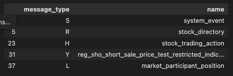
A DataFrame named message_types is processed to create a DataFrame called message_labels. The ‘message_type’ and ‘notes’ columns are selected, missing values are removed, and ‘notes’ is renamed to ‘name’. Next, the code converts text to lowercase, removes the substring ‘message’, eliminates periods, trims whitespace, and replaces spaces with underscores in the ‘name’ column. In the message_labels DataFrame, it is suggested to save it to a CSV file. In the final command, the modified DataFrame is displayed.
message_types.message_type = message_types.message_type.ffill()
message_types = message_types[message_types.name != 'message_type']
message_types.value = (message_types.value
                       .str.lower()
                       .str.replace(' ', '_')
                       .str.replace('(', '')
                       .str.replace(')', ''))
message_types.info()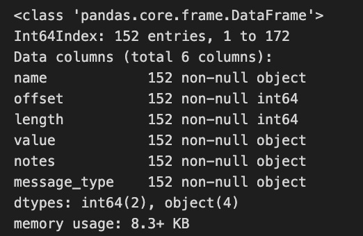
A DataFrame named message_types is manipulated. By using the last valid observation, it fills in any missing values in the message_type column. In the next step, it filters the DataFrame to remove any rows where the name column equals message_type. To standardize data, the value column is converted into lowercase, spaces are replaced with underscores, and parentheses are removed. An overview of the structure and content of the DataFrame is provided by the info method, which gives an overview of the index, column data types, and non-null counts.
message_types.head()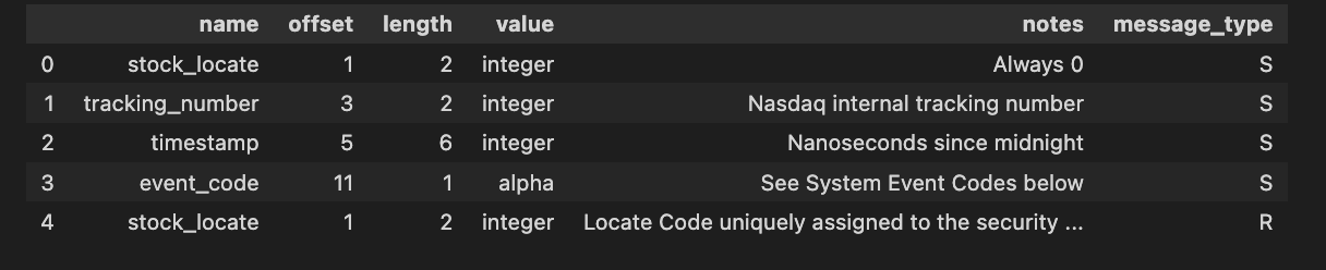
Message_types is retrieved and displayed in this code. In data analysis, it shows column names and data types, along with the data structure. By default, the head function displays the first five rows, which is helpful for understanding the dataset’s format.
Files can be loaded or saved.
message_types.to_csv('message_types.csv', index=False)
message_types = pd.read_csv('message_types.csv')
Code saves message_types.csv, without the row index, from a DataFrame named message_types. In a new DataFrame named message_types, the data is loaded from this file. The DataFrame is written to a file, then read back into memory, allowing data persistence and manipulation.
Message specifications are converted into format strings and namedtuples that define message content. Based on ITCH specifications, formatting tuples with type and length are created.
message_types.loc[:, 'formats'] = (message_types[['value', 'length']]
                            .apply(tuple, axis=1).map(formats))
This code transforms the value and length columns into tuples for each row in message_types DataFrame. A format dictionary or function is then used to look up or calculate the corresponding value from the tuples. Based on the value-length pairs, the format column is assigned the appropriate format on rows.
Alphabetic fields are formatted.
alpha_fields = message_types[message_types.value == 'alpha'].set_index('name')
alpha_msgs = alpha_fields.groupby('message_type')
alpha_formats = {k: v.to_dict() for k, v in alpha_msgs.formats}
alpha_length = {k: v.add(5).to_dict() for k, v in alpha_msgs.length}
DataFrame named message_types is processed to extract alpha message information. Only the rows with the value alpha are included in the DataFrame, and the index is set to name. By creating a group for each unique message type, the code groups the filtered DataFrame by message_type. In alpha_formats, each message type is mapped to its corresponding format, while in alpha_length, each message length is added to 5 before being converted into a dictionary. Alpha message formats and lengths are organized and enhanced in this code.
message_fields, fstring = {}, {}
for t, message in message_types.groupby('message_type'):
    message_fields[t] = namedtuple(typename=t, field_names=message.name.tolist())
    fstring[t] = '>' + ''.join(message.formats.tolist())
DataFrame message_types contains information about various message types. Each unique message type is created as a group in the DataFrame. Each group is represented by a named tuple generated by namedtuple. Field names in the named tuples are derived from the names in the name column of the message DataFrame, allowing direct access to message fields.
Similarly, the code concatenates the formats from the formats column without spaces, starting with a greater-than character. As a message type identifier, this string serves as a format. Each message type’s message fields are stored in message_fields, while its format string stores its format information.
def format_alpha(mtype, data):
    """Process byte strings of type alpha"""

    for col in alpha_formats.get(mtype).keys():
        if mtype != 'R' and col == 'stock':
            data = data.drop(col, axis=1)
            continue
        data.loc[:, col] = data.loc[:, col].str.decode("utf-8").str.strip()
        if encoding.get(col):
            data.loc[:, col] = data.loc[:, col].map(encoding.get(col))
    return data
A DataFrame containing the byte strings should be passed to the format_alpha function as data and mtype, which specifies the formatting. Ititerates over alpha_formats’ keys after retrieving a dictionary with mtype. DataFrame columns named stock that are not R types are removed. It decodes other columns from UTF-8 and removes any leading or trailing whitespace. This function further transforms decoded values if the encoding dictionary contains a corresponding mapping. A modified DataFrame is returned by the function.
There are over 350 million messages in one day’s binary file.
def store_messages(m):
    """Handle occasional storing of all messages"""
    with pd.HDFStore(itch_store) as store:
        for mtype, data in m.items():
            # convert to DataFrame
            data = pd.DataFrame(data)

            # parse timestamp info
            data.timestamp = data.timestamp.apply(int.from_bytes, byteorder='big')
            data.timestamp = pd.to_timedelta(data.timestamp)

            # apply alpha formatting
            if mtype in alpha_formats.keys():
                data = format_alpha(mtype, data)

            s = alpha_length.get(mtype)
            if s:
                s = {c: s.get(c) for c in data.columns}
            dc = ['stock_locate']
            if m == 'R':
                dc.append('stock')
            store.append(mtype,
                         data,
                         format='t',
                         min_itemsize=s,
                         data_columns=dc)
Pandas library is used to store messages in HDF5 format. The dictionary is composed of keys representing message types and values representing associated data. By converting each message type to a pandas DataFrame, the function opens an HDF5 store. Analyzing timestamps requires converting bytes to integers and converting them into a time delta format.
Message types that have specific formatting are applied to data. Optimizes the storage structure by checking minimum item sizes. Indexing is done by adding columns to data_columns. Lastly, HDF5 stores the processed DataFrame under the appropriate message type, ensuring optimal data storage.
messages = {}
message_count = 0
message_type_counter = Counter()
Initializes message handling variables. The Messages dictionary stores individual messages as keys with unique identifiers. The message count is set to zero, which tracks the total number of messages. The message type counter is an instance of Counter from the collections module and is used to count different types of messages. Using these variables, messages can be managed and analyzed systematically.
start = time()
with file_name.open('rb') as data:
    while True:

        # determine message size in bytes
        message_size = int.from_bytes(data.read(2), byteorder='big', signed=False)

        # get message type by reading first byte
        message_type = data.read(1).decode('ascii')

        # create data structure to capture result
        if not messages.get(message_type):
            messages[message_type] = []

        message_type_counter.update([message_type])

        # read & store message
        record = data.read(message_size - 1)
        message = message_fields[message_type]._make(unpack(fstring[message_type], record))
        messages[message_type].append(message)

        # deal with system events
        if message_type == 'S':
            timestamp = int.from_bytes(message.timestamp, byteorder='big')
            print('\n', event_codes.get(message.event_code.decode('ascii'), 'Error'))
            print('\t{0}\t{1:,.0f}'.format(timedelta(seconds=timestamp * 1e-9),
                                         message_count))
            if message.event_code.decode('ascii') == 'C':
                store_messages(messages)
                break

        message_count += 1
        if message_count % 2.5e7 == 0:
            timestamp = int.from_bytes(message.timestamp, byteorder='big')
            print('\t{0}\t{1:,.0f}\t{2}'.format(timedelta(seconds=timestamp * 1e-9),
                                                message_count,
                                                timedelta(seconds=time() - start)))
            store_messages(messages)
            messages = {}


print(timedelta(seconds=time() - start))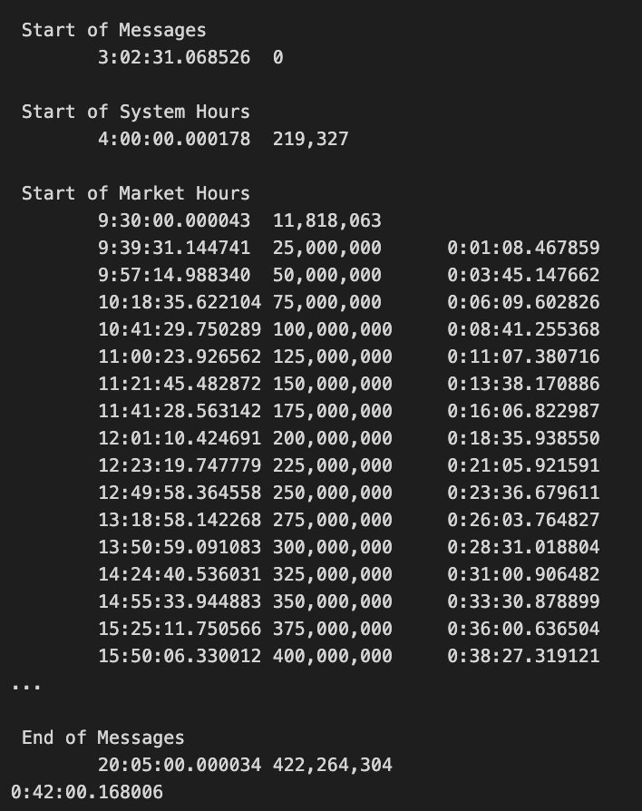
This code snippet measures performance by looping through binary files. A binary read mode is opened and messages are continuously read with a two-byte size indicator. The next byte specifies the message type, which is decoded to ASCII characters. In the message dictionary, a new entry is created for each new message type.
Based on the message size, the counter for message types is updated. Based on a predefined format, unpack structures the message contents. Messages indicating system events with the letter S are extracted and a timestamp, along with an event code, are printed. If the event code is C, it triggers a function to store messages and exits the loop.
The code also tracks the number of messages processed and prints the elapsed time every 25 million messages, storing them and clearing the messages dictionary. Finally, it outputs the total elapsed time once the loop completes.
counter = pd.Series(message_type_counter).to_frame('# Trades')
counter['Message Type'] = counter.index.map(message_labels.set_index('message_type').name.to_dict())
counter = counter[['Message Type', '# Trades']].sort_values('# Trades', ascending=False)
print(counter)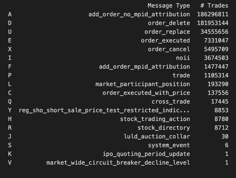
An occurrence counter named message_type_counter is created from a pandas DataFrame named message_type_counter. # Trades column is added to the DataFrame. After mapping message type labels to message_labels, it creates Message Type, using message_type as the key. A dictionary is created with message_types as keys and names as values for message_labels. An index of the counter DataFrame is mapped. This code restructures the DataFrame to only include the Message Type and # Trades columns, and then sorts it descendingly by # Trades before printing the result. This allows us to easily see which message types have the most trades.
with pd.HDFStore(itch_store) as store:
    store.put('summary', counter)
The Pandas library is used to work with HDF5 files, which are suitable for storing large datasets in a hierarchical format. By calling pd.HDFStore, you can connect to the HDF5 file specified by itch_store. Assuring that operations are completed correctly is achieved with the with statement. Variable counters are stored under the key summary of the HDF5 file using the store.put function. In addition, the with statement avoids unintentionally leaving file handles open.
with pd.HDFStore(itch_store) as store:
    stocks = store['R'].loc[:, ['stock_locate', 'stock']]
    trades = store['P'].append(store['Q'].rename(columns={'cross_price': 'price'}), sort=False).merge(stocks)
trades['value'] = trades.shares.mul(trades.price)
trades['value_share'] = trades.value.div(trades.value.sum())
trade_summary = trades.groupby('stock').value_share.sum().sort_values(ascending=False)
trade_summary.iloc[:50].plot.bar(figsize=(14, 6), color='darkblue', title='Share of Traded Value')
plt.gca().yaxis.set_major_formatter(FuncFormatter(lambda y, _: '{:.0%}'.format(y)))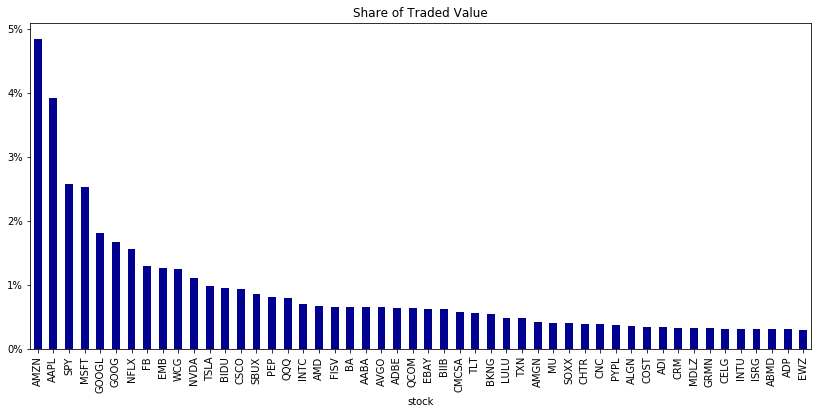
Using pd.HDFStore, this code reads and manipulates HDF5 trading data. There are two datasets extracted: stocks that contain stock identifiers and trades that combine P and Q. After renaming the cross_price column to price, the Q dataset is merged with stocks to associate stock information with trades.
By multiplying the number of shares by the price, the code calculates each trade’s value. By dividing individual trade values by total trade values, it calculates the value share of each trade.
We sum the value share of the trading data by stock. A dark blue color scheme and a specified figure size enhance clarity in this bar chart of the top 50 stocks by traded value share. Y-axis displays percentages.
stock = 'AAPL'
order_dict = {-1: 'sell', 1: 'buy'}
The stock variable in this program is initialized with AAPL, the stock symbol for Apple Inc. A dictionary named order_dict is also created, where the key -1 corresponds to the action sell and key 1 corresponds to the action buy. Trading applications benefit from this structure, as it helps determine whether to buy or sell a stock.
def get_messages(date, stock=stock):
    """Collect trading messages for given stock"""
    with pd.HDFStore(itch_store) as store:
        stock_locate = store.select('R', where='stock = stock').stock_locate.iloc[0]
        target = 'stock_locate = stock_locate'

        data = {}
        # trading message types
        messages = ['A', 'F', 'E', 'C', 'X', 'D', 'U', 'P', 'Q']
        for m in messages:
            data[m] = store.select(m, where=target).drop('stock_locate', axis=1).assign(type=m)

    order_cols = ['order_reference_number', 'buy_sell_indicator', 'shares', 'price']
    orders = pd.concat([data['A'], data['F']], sort=False, ignore_index=True).loc[:, order_cols]

    for m in messages[2: -3]:
        data[m] = data[m].merge(orders, how='left')

    data['U'] = data['U'].merge(orders, how='left',
                                right_on='order_reference_number',
                                left_on='original_order_reference_number',
                                suffixes=['', '_replaced'])

    data['Q'].rename(columns={'cross_price': 'price'}, inplace=True)
    data['X']['shares'] = data['X']['cancelled_shares']
    data['X'] = data['X'].dropna(subset=['price'])

    data = pd.concat([data[m] for m in messages], ignore_index=True, sort=False)
    data['date'] = pd.to_datetime(date, format='%m%d%Y')
    data.timestamp = data['date'].add(data.timestamp)
    data = data[data.printable != 0]

    drop_cols = ['tracking_number', 'order_reference_number', 'original_order_reference_number',
                 'cross_type', 'new_order_reference_number', 'attribution', 'match_number',
                 'printable', 'date', 'cancelled_shares']
    return data.drop(drop_cols, axis=1).sort_values('timestamp').reset_index(drop=True)
This function returns trading messages for a given stock. HDF5 stores records by stock identifiers. Messaging types are listed in the dictionary. The new column for message types identifies relevant trading messages by excluding stock_locate.
Columns selected for analysis are from message types A and F. The details are merged into other message types, especially for messages U. Renaming column Q and adjusting share data for message X removes rows without prices.
Timestamps are adjusted to match the specified date after merging DataFrames. Remove rows marked as unprintable. A cleaned DataFrame is returned for further analysis after we drop non-essential columns.
messages = get_messages(date=date)
messages.info(null_counts=True)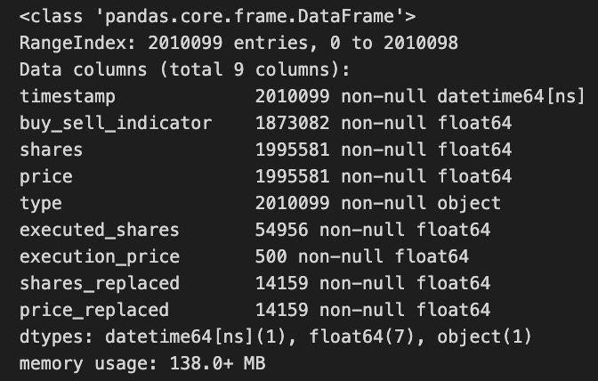
A data source filtered by a specific date is used to retrieve messages, which are stored in the messages variable. The info method is then called on the messages object to provide a summary of its contents. This allows for an assessment of data completeness by showing null_counts=True for each column.
with pd.HDFStore(order_book_store) as store:
    key = '{}/messages'.format(stock)
    store.put(key, messages)
    print(store.info())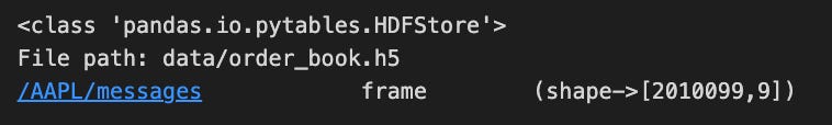
A pandas library is used to store stock-related messages in an HDF5 file. This function opens the HDF5 file order_book_store within the context manager so that it can be handled properly. With the stock identifier and the string messages, the code constructs a unique variable called key. A store.put() method is used to save the messages data in the HDF5 file. To verify that the data was successfully added and provide details about the data structure, the code prints information about HDF5 store contents.
def get_trades(m):
    """Combine C, E, P and Q messages into trading records"""
    trade_dict = {'executed_shares': 'shares', 'execution_price': 'price'}
    cols = ['timestamp', 'executed_shares']
    trades = pd.concat([m.loc[m.type == 'E', cols + ['price']].rename(columns=trade_dict),
                        m.loc[m.type == 'C', cols + ['execution_price']].rename(columns=trade_dict),
                        m.loc[m.type == 'P', ['timestamp', 'price', 'shares']],
                        m.loc[m.type == 'Q', ['timestamp', 'price', 'shares']].assign(cross=1),
                        ], sort=False).dropna(subset=['price']).fillna(0)
    return trades.set_index('timestamp').sort_index().astype(int)
Using a DataFrame containing a type column, this function compiles trading records. It starts by mapping executed share and price column names. It selects and renames relevant columns based on message types: executions, cancellations, prices, and quotes. With pd.concat, these subsets are combined into one DataFrame.
Then it removes rows without a price value, fills missing values with zeros, and sorts records chronologically by timestamp. All numeric values are then converted to integers and the trading data is returned.
trades = get_trades(messages)
print(trades.info())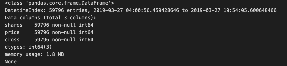
This code calls the get_trades function with a variable named messages to retrieve trade data from the trades variable. Using the info method, it prints a summary of the trades DataFrame, including the number of entries, column data types, and memory usage details, so that users can quickly understand the structure and content.
with pd.HDFStore(order_book_store) as store:
    store.put('{}/trades'.format(stock), trades)
For storing large amounts of data, this code uses the pandas library. By opening an HDF5 file in the context manager, it ensures that the file is properly closed after operations. As part of this context, it creates a path stock/trades in the HDF5 file by saving a DataFrame representing trades. By organizing trades by stock, future retrievals are easier.
def add_orders(orders, buysell, nlevels):
    """Add orders up to desired depth given by nlevels;
        sell in ascending, buy in descending order
    """
    new_order = []
    items = sorted(orders.copy().items())
    if buysell == 1:
        items = reversed(items)
    for i, (p, s) in enumerate(items, 1):
        new_order.append((p, s))
        if i == nlevels:
            break
    return orders, new_order
Orders, buysell, and nlevels are the parameters for add_orders. In this function, nlevels is used to determine how many order levels should be added to the existing order list.
To maintain the original data, the function starts with an empty list called new_order. Sorting by price organizes the orders. Depending on buysell, the sorted items may be reversed. It processes prices ascendingly for selling, and descendingly for buying if buysell equals 1.
As the function iterates over the sorted items, it adds each price and size to the new_order list until it reaches the specified nlevels, ensuring that no more orders are added than necessary. In addition, the function returns a tuple including the original orders and the newly created new_order list, so other parts of the code can understand the changes.
def save_orders(orders, append=False):
    cols = ['price', 'shares']
    for buysell, book in orders.items():
        df = (pd.concat([pd.DataFrame(data=data,
                                     columns=cols)
                         .assign(timestamp=t)
                         for t, data in book.items()]))
        key = '{}/{}'.format(stock, order_dict[buysell])
        df.loc[:, ['price', 'shares']] = df.loc[:, ['price', 'shares']].astype(int)
        with pd.HDFStore(order_book_store) as store:
            if append:
                store.append(key, df.set_index('timestamp'), format='t')
            else:
                store.put(key, df.set_index('timestamp'))
HDF5 file format efficiently handles large datasets, which is used by save_orders to store order data. Data is appended or overwritten depending on the boolean flag.
In the function, price and shares are defined as columns. DataFrames are created for each buy or sell action, and timestamps linked to each order are concatenated into a single DataFrame.
An order type and stock identifier are combined into a unique key for the dataset. Consistency and space-saving are achieved by converting price and shares columns to integers.
The function then opens an HDF5 store and either appends or creates a new dataset based on the value of append. Pd.HDFStore ensures proper resource management by closing the store after operations are completed, indexing both datasets by timestamp.
order_book = {-1: {}, 1: {}}
current_orders = {-1: Counter(), 1: Counter()}
message_counter = Counter()
nlevels = 100

start = time()
for message in messages.itertuples():
    i = message[0]
    if i % 1e5 == 0 and i > 0:
        print('{:,.0f}\t\t{}'.format(i, timedelta(seconds=time() - start)))
        save_orders(order_book, append=True)
        order_book = {-1: {}, 1: {}}
        start = time()
    if np.isnan(message.buy_sell_indicator):
        continue
    message_counter.update(message.type)

    buysell = message.buy_sell_indicator
    price, shares = None, None

    if message.type in ['A', 'F', 'U']:
        price = int(message.price)
        shares = int(message.shares)

        current_orders[buysell].update({price: shares})
        current_orders[buysell], new_order = add_orders(current_orders[buysell], buysell, nlevels)
        order_book[buysell][message.timestamp] = new_order

    if message.type in ['E', 'C', 'X', 'D', 'U']:
        if message.type == 'U':
            if not np.isnan(message.shares_replaced):
                price = int(message.price_replaced)
                shares = -int(message.shares_replaced)
        else:
            if not np.isnan(message.price):
                price = int(message.price)
                shares = -int(message.shares)

        if price is not None:
            current_orders[buysell].update({price: shares})
            if current_orders[buysell][price] <= 0:
                current_orders[buysell].pop(price)
            current_orders[buysell], new_order = add_orders(current_orders[buysell], buysell, nlevels)
            order_book[buysell][message.timestamp] = new_order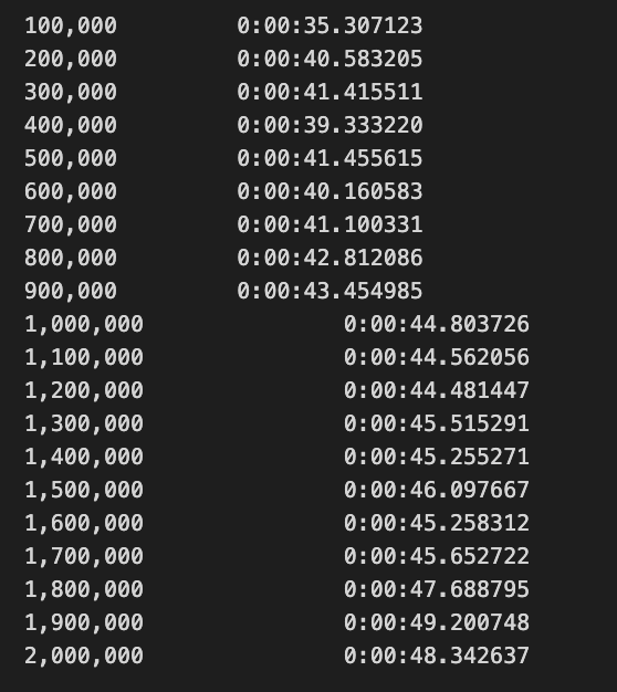
To update a buy and sell order book, this code processes trading messages. Order_book tracks active orders and current_orders counts shares at various price levels. Received messages are tallied by message_counter.
Processing begins with a timer to enable periodic progress updates. Code iterates through messages and reports the current count and processing time after every 100,000 messages, saves the order book’s state, and resets it for the next batch.
Each message checks the buy_sell_indicator. Messages typed A, F, or U are adds, modifications, or updates, which retrieve the price and number of shares, respectively, and update current_orders. New orders are stored in order_book indexed by timestamp by the function add_orders.
Current_orders are adjusted based on price and shares for message types indicating edits or cancellations, such as E, C, X, D, or U. When shares are replaced or cancelled, shares can be set to negative values or orders can be removed.
The code dynamically responds to incoming trade messages to reflect the latest information on open trading orders.
