Algorithmic Trading: Chapter 2 — Normalizing and Analyzing Market Data

A Comprehensive Guide to Data Normalization, Analysis, and Visualization Techniques in Algorithmic Trading

Sep 05, 2024

∙ Paid

In Chapter 2 of the Algorithmic Trading series, we delve into the essential processes of normalizing and analyzing market data. This chapter provides a step-by-step guide on how to prepare, manipulate, and visualize financial data using Python. By leveraging powerful libraries such as Pandas, NumPy, and Matplotlib, traders can efficiently handle large datasets, perform statistical analysis, and create insightful visualizations. These techniques are crucial for developing and refining trading strategies based on robust and reliable data analysis.

Source code at the end of this article!

import pandas as pd
from pathlib import Path
import numpy as np
from collections import Counter
from time import time
from datetime import datetime, timedelta, time
import seaborn as sns
import matplotlib as mpl
import matplotlib.pyplot as plt
from matplotlib.ticker import FuncFormatter
from math import pi
from bokeh.plotting import figure, show, output_file, output_notebook
from scipy.stats import normaltest

Statistical analysis, data manipulation, and visualization are all supported in this code snippet. To create and manage data frames, Pandas is imported as pd. File path operations can be handled with the Path class from pathlib. Mathematical computations are made easier with Numpy, especially for handling arrays. The collections module counts hashable objects to aid frequency analysis. Time functions are handled by the time module; dates and times are handled by datetime. Python uses seaborn, matplotlib, and pyplot module for creating various types of visualizations. Formatting tick labels in plots is customizable with FuncFormatter. Mathematical functions, especially those involving constants, are supported in the library. Interactive visualizations in web browsers or notebooks are created with Bokeh. A normal distribution is a crucial requirement for many statistical analysis, as checked by normaltest in scipy.stats. Data analysis, manipulation, and visualization tasks can be performed with these imports.

%matplotlib inline
pd.set_option('display.float_format', lambda x: '%.2f' % x)
plt.style.use('fivethirtyeight')

First line enables matplotlib plots to display directly in Jupyter notebooks, improving interaction with visualizations. Two decimal places are formatted in the second line for better readability in pandas dataframes. FiveThirtyEight’s data journalism site uses a visually appealing design consistent with the final line of the plotting style.

data_path = Path('data')
itch_store = str(data_path / 'itch.h5')
order_book_store = str(data_path / 'order_book.h5')
stock = 'AAPL'
date = '20190327'
title = '{} | {}'.format(stock, pd.to_datetime(date).date())

This code loads financial data for a specific stock on a designated date. Path objects are created for data directories, which store data files. In the data directory, itch.h5 and order_book.h5 are assigned paths by joining itch_store and order_book_store variables together. In this example, Apple Inc is represented by AAPL and March 27, 2019 is represented by 20190327. For display purposes or reports, title accepts AAPL as a stock ticker and formats the date as a readable format using pd.to_datetime().

with pd.HDFStore(itch_store) as store:
    sys_events = store['S'].set_index('event_code').drop_duplicates()
    sys_events.timestamp = sys_events.timestamp.add(pd.to_datetime(date)).dt.time
    market_open = sys_events.loc['Q', 'timestamp']
    market_close = sys_events.loc['M', 'timestamp']

To retrieve and process system event data, this code snippet interacts with Pandas HDF5. Using a context manager, it ensures the HDF5 file specified by itch_store is handled and closed properly. Once open, the ‘S’ dataset is accessed, the ‘event_code’ column indexed, and duplicate entries removed. A specified date is then added to the ‘timestamp’ column to convert the timestamps into valid time objects. Market_open captures ‘Q’ for market opening and market_close captures ‘M’ for market closing timestamps.

with pd.HDFStore(itch_store) as store:
    stocks = store['R']
stocks.info()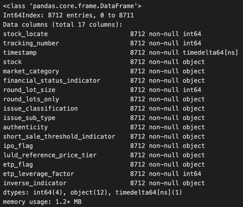

In this code snippet, the pandas library opens and loads a dataset stored under the key R from an HDF5 file. By closing the connection when the block ends, the with statement ensures proper HDFStore management. Stocks’ info method is called after the data is loaded to provide a summary of the DataFrame’s structure, including the number of entries, column names, and data types. Using this summary, one can quickly understand the DataFrame’s shape and type.

with pd.HDFStore(itch_store) as store:
    stocks = store['R'].loc[:, ['stock_locate', 'stock']]
    trades = store['P'].append(store['Q'].rename(columns={'cross_price': 'price'}), sort=False).merge(stocks)

trades['value'] = trades.shares.mul(trades.price)    
trades['value_share'] = trades.value.div(trades.value.sum())
trade_summary = trades.groupby('stock').value_share.sum().sort_values(ascending=False)
trade_summary.iloc[:50].plot.bar(figsize=(14, 6), color='darkblue', title='% of Traded Value')
plt.gca().yaxis.set_major_formatter(FuncFormatter(lambda y, _: '{:.0%}'.format(y)))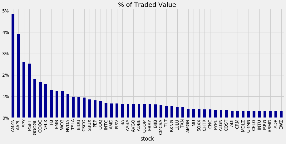

A Pandas library is used to analyze trading data in an HDF5 file. This opens an HDF5 store with trading data for a stock in three tables: R for stock information and P and Q for trade data. In this code, the relevant stock data is retrieved, the trade data is merged from P and Q, and a column in Q is renamed. The value of each trade is calculated by multiplying the number of shares by the trade price and computing a value share based on the trade’s proportion to the total value.

Summing the value share of each stock and sorting the results in descending order summarizes the data. For a clear comparison of each stock’s traded value, the y-axis displays percentages to display the top 50 stocks by traded value share.

with pd.HDFStore(order_book_store) as store:
    trades = store['{}/trades'.format(stock)]

This code snippet interacts with an HDF5 file, a format for storing large datasets that is efficient. The HDF5 file is opened by order_book_store with the HDFStore context manager. By using string formatting, it dynamically creates the dataset path for the trades dataset for a specific stock. You can now analyze or process the data from the trades variable.

trades.price = trades.price.mul(1e-4)
trades = trades[trades.cross == 0]
trades = trades.between_time(market_open, market_close).drop('cross', axis=1)
trades.info()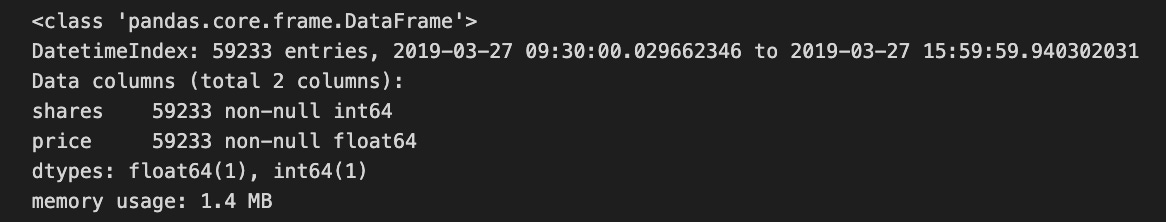

A DataFrame named trades is processed by this code. It multiplies the prices by 0.0001 to scale them down. This filter retains only the rows that have a cross value of zero, indicating that these trades do not exceed certain thresholds. In addition, only trades that took place between market_open and market_close are included in the data. Lastly, cross is removed from the DataFrame since it is no longer needed. It displays the number of entries, the data type of each column, and the structure of the DataFrame.

tick_bars = trades.copy()
tick_bars.index = tick_bars.index.time
tick_bars.price.plot(figsize=(10, 5), title='{} | {}'.format(stock, pd.to_datetime(date).date()), lw=1)
plt.xlabel('')
plt.tight_layout();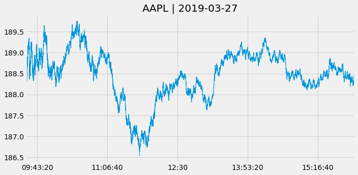

By copying the trades DataFrame and removing the date component, this code creates a new DataFrame named tick_bars. Using tick_bars, it plots the price column with a figure size of 10 by 5 inches and a title that includes both the stock name and the date. To improve visual clarity, plt.tight_layout() is called to set the plot line width and remove the x-axis label.

normaltest(tick_bars.price.pct_change().dropna())

A normality test is performed on the tick_bars dataset’s percentage changes in price values. A percentage change between consecutive price entries can be calculated using tick_bars.price.pct_change(), while any NaN values from this calculation can be removed by dropna(). By returning a statistic and a p-value, normaltest() tests for the null hypothesis that the data follow a normal distribution. Analysis or modeling can benefit from this information.

def price_volume(df, price='vwap', vol='vol', suptitle=title):
    
    fig, axes = plt.subplots(nrows=2, sharex=True, figsize=(15,8))
    axes[0].plot(df.index, df[price])
    axes[1].bar(df.index, df[vol], width=1/(len(df.index)), color='r')
    
    # formatting
    xfmt = mpl.dates.DateFormatter('%H:%M')
    axes[1].xaxis.set_major_locator(mpl.dates.HourLocator(interval=3))
    axes[1].xaxis.set_major_formatter(xfmt)
    axes[1].get_xaxis().set_tick_params(which='major', pad=25)
    axes[0].set_title('Price', fontsize=14)
    axes[1].set_title('Volume', fontsize=14)
    fig.autofmt_xdate()
    fig.suptitle(suptitle)
    fig.tight_layout()
    plt.subplots_adjust(top=0.9)

Price and volume data are visualized using Matplotlib’s price_volume function. Two vertically stacked subplots appear in the figure: the first displays price data, typically the VWAP price, while the second displays volume data in a bar chart, using the vol column.

Using this function, the layout can be configured to share the x-axis. The time-based x-axis makes use of a date formatter, with major ticks every three hours. The layout is adjusted to ensure proper spacing and fit for subplots and a main title for the figure.

The function aids in analyzing and interpreting data over time by displaying price and volume changes.

def get_bar_stats(agg_trades):
    vwap = agg_trades.apply(lambda x: np.average(x.price, weights=x.shares)).to_frame('vwap')
    ohlc = agg_trades.price.ohlc()
    vol = agg_trades.shares.sum().to_frame('vol')
    txn = agg_trades.shares.size().to_frame('txn')
    return pd.concat([ohlc, vwap, vol, txn], axis=1)

The function get_bar_stats computes key trading statistics based on agg_trades, a DataFrame containing aggregated trading data. Volume-Weighted Average Price is calculated by averaging price weighted by number of shares, producing a new DataFrame with a column named vwap. To summarize price movements, it also generates Open, High, Low, Close (OHLC). By summing all shares traded, the function calculates total trading volume. Furthermore, it stores the number of transactions in a DataFrame named txn by determining the size of the shares series. To provide a comprehensive summary of trading statistics, each DataFrame for OHLC, vwap, vol, and txn is combined using pd.concat.

resampled = trades.resample('1Min')
time_bars = get_bar_stats(resampled)
normaltest(time_bars.vwap.pct_change().dropna())

Three steps are involved in this code. By resampling the trade data, it aggregates the data for minute-by-minute analysis. The volume-weighted average price for each minute is computed by calling get_bar_stats on the resampled data. In the end, the VWAP percentage changes are tested for normality. A percentage change between consecutive values is calculated, missing data is removed, and the distribution of these changes is evaluated to see if it deviates significantly from normality.

Continue reading this post for free, courtesy of Onepagecode.

Or purchase a paid subscription.