

Algorithmic Trading using Deep Autoencoder based Statistical Arbitrage
In the world of finance, the fusion of technology and trading strategies has opened up new frontiers for investors and traders alike.

Among these, algorithmic trading and deep learning stand out as two pivotal innovations reshaping how financial markets operate. Before we explore the intricate world of using deep autoencoders for statistical arbitrage in algorithmic trading, let’s demystify some core concepts and lay a foundation for everyone, regardless of their prior knowledge.
Download the source code from the link at the end of this article.
What is Algorithmic Trading?
Algorithmic trading, at its core, involves using computer algorithms to execute trading orders at speeds and volumes that are humanly unachievable. These algorithms are designed to identify trading opportunities based on market data, statistical models, and quantitative analysis, aiming to maximize profits and reduce risks. From executing simple trades to managing complex portfolios, algorithmic trading leverages the power of computation to navigate the financial markets efficiently.
The Role of Deep Learning in Finance
Deep learning, a subset of machine learning, mimics the workings of the human brain in processing data and creating patterns for use in decision-making. It uses structures called neural networks with many layers (hence “deep”) to analyze vast amounts of data, learn from them, and make predictions or decisions without being explicitly programmed for the task. In finance, deep learning can predict stock prices, identify trading signals, and even uncover insights into market trends that are not immediately obvious to human analysts.
Introducing Deep Autoencoders
Deep autoencoders are a type of neural network used for learning efficient representations (encodings) of data, primarily for the purpose of dimensionality reduction or feature learning. They consist of two main parts: an encoder that reduces the input data into a smaller, dense representation, and a decoder that reconstructs the data from this representation. This ability makes them particularly useful in financial markets, where they can identify complex, non-linear patterns in price data, helping traders to devise sophisticated trading strategies.
Preparing for a Deep Dive into Algorithmic Trading
Understanding the basics of algorithmic trading and deep learning requires familiarity with certain concepts and tools. Python, a versatile programming language, is a favorite in the financial and data science communities for its simplicity and powerful libraries like NumPy, pandas, and TensorFlow. Knowledge of these tools, along with basic financial terminologies — such as stocks, portfolios, returns, and risk — will be instrumental as we explore the application of deep autoencoders in trading.
Bridging the Gap
As we venture into the realm of applying deep autoencoders for statistical arbitrage — a strategy that leverages price inefficiencies across similar assets — it’s important to approach the subject with a blend of curiosity and caution. The intersection of finance and deep learning is rich with opportunities but also riddled with complexities. Our goal is to demystify these complexities, making advanced trading strategies accessible and understandable to all.
Analyzing stock price using moving averages.
import numpy as np
import pandas as pd
import matplotlib.pyplot as plt
import math
%matplotlib inline
xl_aapl = pd.ExcelFile('/dli/tasks/task3/task/data/AAPL.xlsx')
dfP_aapl = xl_aapl.parse('Sheet1')
P_aapl = dfP_aapl.fillna(method="backfill")
P_aapl = np.array(P_aapl.drop('Date', axis=1))
W_LTMA = 60
W_STMA = 30
T1_aaple = 0.03
T2_aaple = 0.01
[R_aaple, C_aaple] = P_aapl.shape
dm = np.zeros(shape=(R_aaple-W_LTMA,3), dtype=float)
mr = np.zeros(shape=(R_aaple-W_LTMA,1), dtype=float)
pos_aaple = np.zeros(shape=(R_aaple-W_LTMA+1,1), dtype=int)
p_apple_snap = 0.0
PNL_apple = np.zeros(shape=(R_aaple-W_LTMA,1), dtype=float)
idx = 0
for i in range(W_LTMA, R_aaple):
    ps = P_aapl[i-W_LTMA:i]
    pf = P_aapl[i-W_STMA:i]
    ms = np.mean(ps)
    mf = np.mean(pf)

    dm[idx,0] = P_aapl[i]
    dm[idx,1] = ms
    dm[idx,2] = mf
    mr[idx] = (mf/ms) - 1

    if pos_aaple[idx-1] == 0 and mr[idx] > T1_aaple:
        pos_aaple[idx] = -1
        p_apple_snap = P_aapl[i]
    elif pos_aaple[idx-1] == 0 and mr[idx] < -T1_aaple:
        pos_aaple[idx] = 1
        p_apple_snap = P_aapl[i]
    elif pos_aaple[idx-1] == -1 and mr[idx] < T2_aaple:
        pos_aaple[idx] = 0
        PNL_apple[idx] = -(P_aapl[i] - p_apple_snap)
    elif pos_aaple[idx-1] == 1 and mr[idx] > -T2_aaple:
        pos_aaple[idx] = 0
        PNL_apple[idx] = P_aapl[i] - p_apple_snap
    else:
        pos_aaple[idx] = pos_aaple[idx-1]

    idx += 1

plt_p, = plt.plot(dm[:,0], label='Price')
plt_ltma, = plt.plot(dm[:,1], label='LTMA')
plt_stma, = plt.plot(dm[:,2], label='STMA{}'.format(W_STMA))
plt.legend(handles=[plt_p, plt_ltma, plt_stma])
plt.title('AAPL')
plt.ylabel('$')
plt.xlabel('Days')
plt.show()

plt.plot(mr)
plt.title('AAPL')
plt.ylabel('STMA{}/LTMA'.format(W_STMA))
plt.xlabel('Days')
plt.show()
plt.plot(pos_aaple)
plt.title('AAPL')
plt.ylabel('Position')
plt.xlabel('Days')
plt.show()
plt.plot(np.cumsum(PNL_apple))
plt.title('AAPL')
plt.ylabel('PNL ($)')
plt.xlabel('Days')
plt.show()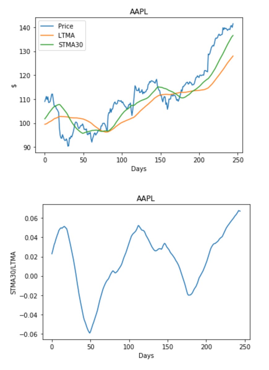
Here is an overview of what the code does:
It utilizes libraries like NumPy, Pandas, and Matplotlib for data manipulation and visualization.
Financial data on Apple stock (‘AAPL.xlsx’) is read from an Excel file into a Pandas DataFrame.
It computes the Long-Term Moving Average (LTMA) and Short-Term Moving Average (STMA) of the stock prices.
Based on specified thresholds (T1_aaple and T2_aaple), it determines whether to initiate a long (buy) or short (sell) position in the stock.
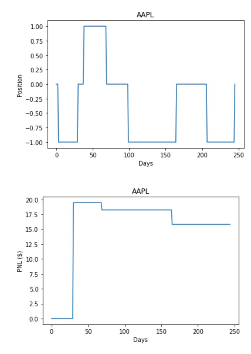
A trading strategy is simulated by taking positions in the stock according to moving average crossovers and calculating the Profit and Loss (PNL) for each trade.
The stock prices, moving averages, trading positions, and PNL are visualized using Matplotlib.
Such trading strategies are employed in financial analysis and algorithmic trading to make buy or sell decisions based on historical data patterns. Visualization aids in understanding the strategy’s performance and pinpointing areas for enhancement.
The code establishes a foundation that can be tailored and improved upon to create more advanced trading algorithms.
Calculates trading strategy for Apple stock.
W_STMA = 20
[R_aaple, C_aaple] = P_aapl.shape
dm = np.zeros(shape=(R_aaple-W_LTMA,3), dtype=float)
mr = np.zeros(shape=(R_aaple-W_LTMA,1), dtype=float)
pos_aaple = np.zeros(shape=(R_aaple-W_LTMA+1,1), dtype=int)
p_apple_snap = 0.0
PNL_apple = np.zeros(shape=(R_aaple-W_LTMA,1), dtype=float)
idx = 0
for i in range(W_LTMA, R_aaple):
    ps = P_aapl[i-W_LTMA:i]
    pf = P_aapl[i-W_STMA:i]
    ms = np.mean(ps)
    mf = np.mean(pf)

    dm[idx,0] = P_aapl[i]
    dm[idx,1] = ms
    dm[idx,2] = mf
    mr[idx] = (mf/ms) - 1

    if pos_aaple[idx-1] == 0 and mr[idx] > T1_aaple:
        pos_aaple[idx] = -1
        p_apple_snap = P_aapl[i]
    elif pos_aaple[idx-1] == 0 and mr[idx] < -T1_aaple:
        pos_aaple[idx] = 1
        p_apple_snap = P_aapl[i]
    elif pos_aaple[idx-1] == -1 and mr[idx] < T2_aaple:
        pos_aaple[idx] = 0
        PNL_apple[idx] = -(P_aapl[i] - p_apple_snap)
    elif pos_aaple[idx-1] == 1 and mr[idx] > -T2_aaple:
        pos_aaple[idx] = 0
        PNL_apple[idx] = P_aapl[i] - p_apple_snap
    else:
        pos_aaple[idx] = pos_aaple[idx-1]

    idx += 1

plt_p, = plt.plot(dm[:,0], label='Price')
plt_ltma, = plt.plot(dm[:,1], label='LTMA')
plt_stma, = plt.plot(dm[:,2], label='STMA{}'.format(W_STMA))
plt.legend(handles=[plt_p, plt_ltma, plt_stma])
plt.title('AAPL')
plt.ylabel('$')
plt.xlabel('Days')
plt.show()

plt.plot(mr)
plt.title('AAPL')
plt.ylabel('STMA{}/LTMA'.format(W_STMA))
plt.xlabel('Days')
plt.show()
plt.plot(pos_aaple)
plt.title('AAPL')
plt.ylabel('Position')
plt.xlabel('Days')
plt.show()
plt.plot(np.cumsum(PNL_apple))
plt.title('AAPL')
plt.ylabel('PNL ($)')
plt.xlabel('Days')
plt.show()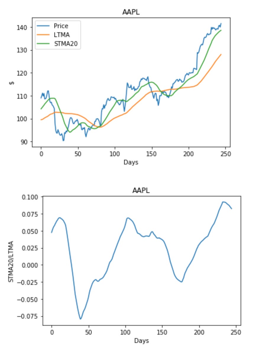
The process involves initializing variables and arrays, calculating short-term and long-term moving averages for the stock prices, determining trade positions based on moving average ratios, calculating profits or losses for each trade, and plotting stock price, moving averages, trade positions, and profits/losses over time. Traders and investors can use this strategy to evaluate its performance and make informed trading decisions regarding AAPL stock based on the generated signals.
The second figure represents a signal that is the ratio of short-term moving average (STMA) to long-term moving average (LTMA). This signal fluctuates around a mean of zero. When the signal falls below -T1, the strategy goes long on the stock anticipating a reversion to normal levels. Conversely, when the signal exceeds T1, the strategy goes short on the stock. The third figure above illustrates the positions opened based on this signal, while the fourth figure displays the profit and loss (P&L).
The success of this strategy relies heavily on hyperparameters like the window size of the STMA and LTMA (W_STMA, W_LTMA), as well as the thresholds for opening (T1) and closing (T2) positions.
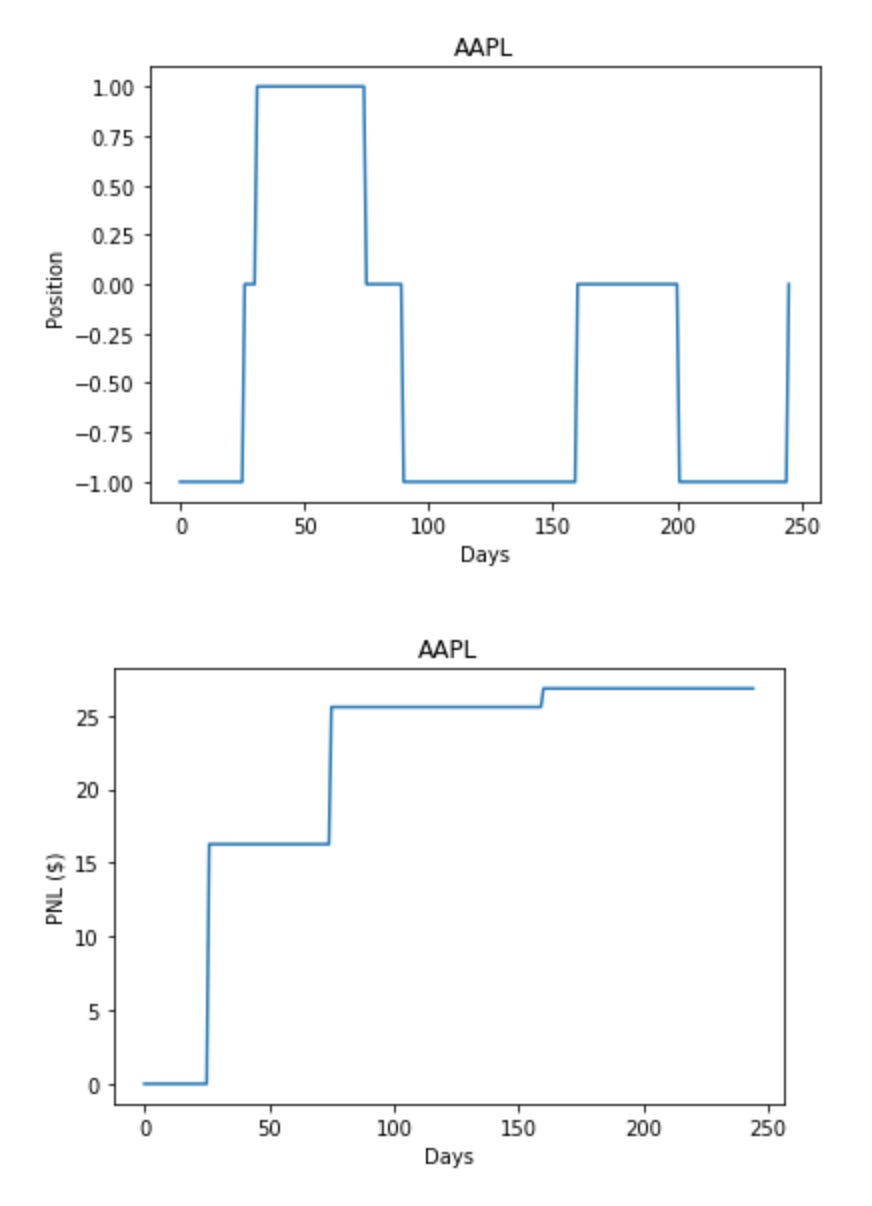
Assuming a short-term average window of W_STMA = 20, rerunning the cell indeed improved the P&L.
While the algorithm is straightforward, fine-tuning hyperparameters can be challenging. Moving average-based mean-reverting strategies were popular in algo-trading during the 1990s but may underperform in certain market conditions such as strong trends. Consequently, strategies like statistical arbitrage (stat-arb) employ sophisticated models to generate more dependable mean-reverting signals for trading.
For those interested in the technical aspects of these methodologies, we recommend referring to the following sources: 2, 3.
An autoencoder is a type of neural network used for unsupervised learning with an architecture that aims to learn efficient data representations in an unsupervised manner.
There is an image named “autoencoder.jpg” with a width of 700px and a height of 900px.
An autoencoder is a type of artificial neural network that is designed to reconstruct its input. It is commonly used in unsupervised learning to learn a compact representation of the input data for dimensionality reduction. The encoder in an autoencoder generates latent features, while the decoder reconstructs the input using these features.
Figure 1 shows diagrams of (a) a basic autoencoder and (b) a deep autoencoder with multiple layers. Autoencoders have gained popularity for learning generative models of data.
The basic architecture of an autoencoder resembles a multilayer perceptron (MLP) with input, output, and hidden layers. The output layer in an autoencoder typically has the same number of nodes as the input layer to reconstruct the original inputs.
Principal component analysis (PCA) is a linear version of an autoencoder and has found widespread applications in industries such as finance and mathematical modeling.
This lab focuses on exploring the performance of deep autoencoders with non-linear activations in the context of statistical arbitrage.
The description of the code for drawing a 5-layer autoencoder has been omitted from the code snippet.
Create and visualize a neural network.
from keras.models import Sequential, Model
from keras.layers import Dense
import nnViz
import matplotlib.pyplot as plt
N_viz = 30
hParams_viz = {}
hParams_viz['inputOutputDimensionality'] = N_viz
hParams_viz['hl1'] = np.int32(N_viz / 2)
hParams_viz['hl2'] = np.int32(hParams_viz['hl1'] / 2)
model_viz = Sequential()
model_viz.add( Dense( hParams_viz['hl1'], input_dim = hParams_viz['inputOutputDimensionality'], activation = 'linear'))
model_viz.add( Dense( hParams_viz['hl2'], activation = 'sigmoid'))
model_viz.add( Dense( hParams_viz['hl1'], activation = 'sigmoid'))
model_viz.add( Dense( hParams_viz['inputOutputDimensionality'], activation = 'linear',))
model_viz.summary()

plt.figure(figsize=(15,15))
nnViz.visualize_model(model_viz)
_________________________________________________________________
Layer (type) Output Shape Param #
=================================================================
dense_29 (Dense) (None, 15) 465
_________________________________________________________________
dense_30 (Dense) (None, 7) 112
_________________________________________________________________
dense_31 (Dense) (None, 15) 120
_________________________________________________________________
dense_32 (Dense) (None, 30) 480
=================================================================
Total params: 1,177
Trainable params: 1,177
Non-trainable params: 0
_________________________________________________________________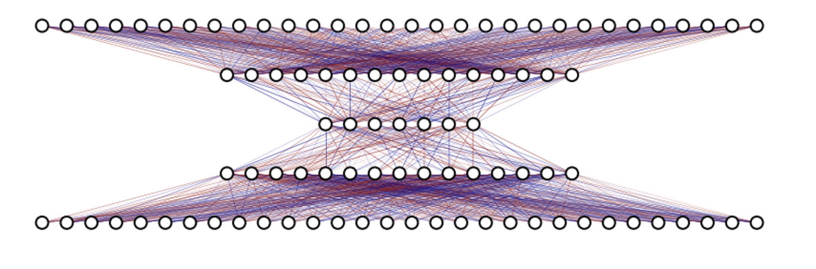
This snippet creates a neural network model using the Keras library. Here’s a breakdown of its functionality:
It imports necessary modules like Sequential, Dense, nnViz, and matplotlib.pyplot for visualization.
Defines parameters for the neural network visualization.
Creates a Sequential model and adds Dense layers with specified activation functions and number of nodes.
Prints a summary of the model architecture.
Sets a figure size for the plot.
Visualizes the neural network model using nnViz.
