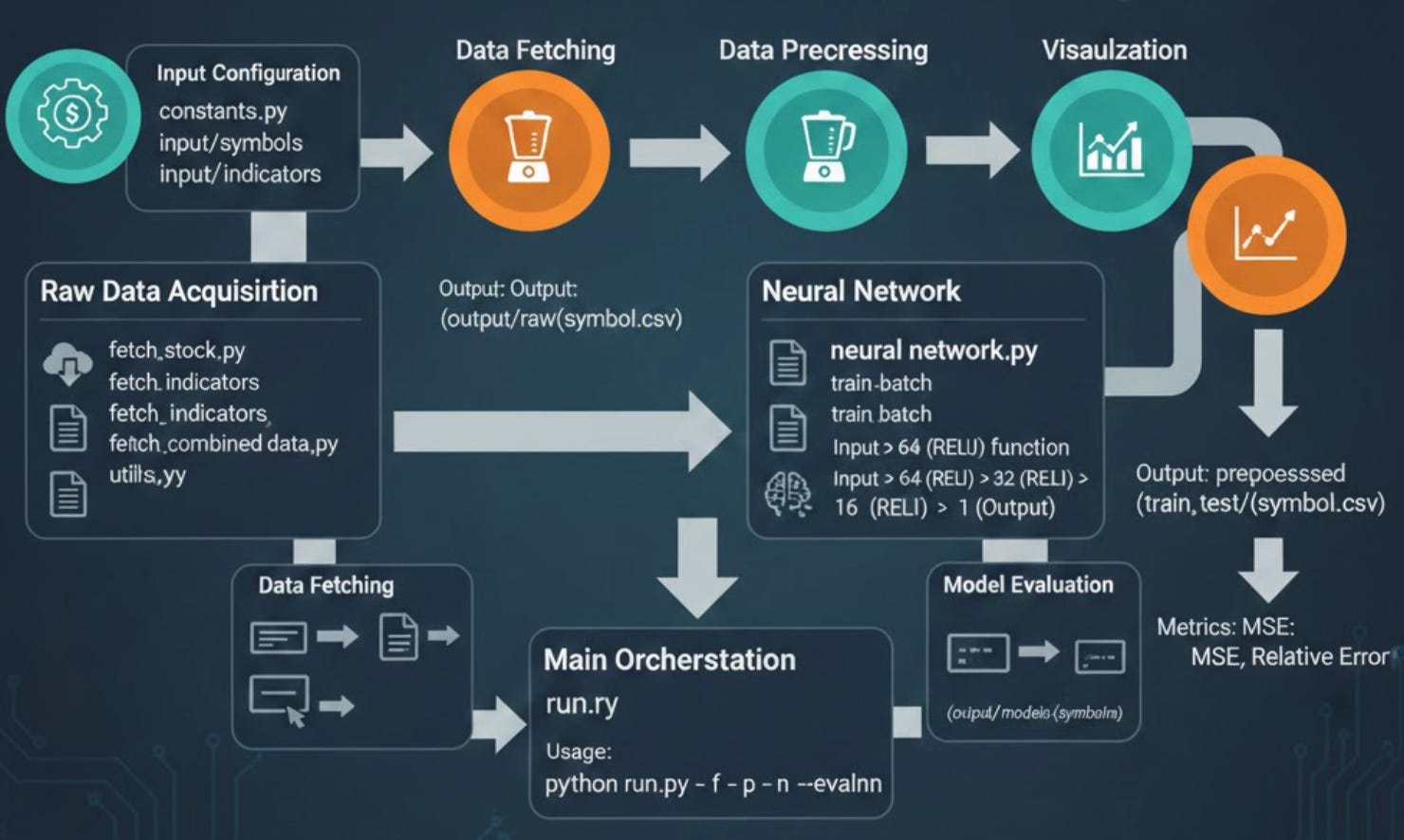
An Algo Trading Framework Using TensorFlow and Alpha Vantage

Building a Scalable Multi-Layer Perceptron Pipeline for Automated Market Analysis

Dec 20, 2025

∙ Paid

Download source code using the button at the end of this article!

Modern financial markets move at a velocity that exceeds human cognitive limits, necessitating a shift toward systematic, data-driven strategies. This project implements an end-to-end algo trading infrastructure designed to bridge the gap between raw market data and actionable intelligence. By leveraging the Alpha Vantage API for real-time price and technical indicator ingestion, the system utilizes a multi-layer perceptron (MLP) neural network to decode non-linear patterns within the noise of daily fluctuations. From automated data cleaning and MinMax normalization to batch model evaluation, this framework provides a robust foundation for developing and backtesting high-frequency predictive models.

File: constants.py

Constants module for the stock prediction application. This module defines all configuration constants used by the fetch script to interact with the Alpha Vantage API. It includes API endpoint configuration, authentication credentials, technical indicator parameters, and data format specifications. These constants are centralized here to allow easy modification and consistent usage across the application.

BASEURL = ‘https://www.alphavantage.co/query?’
API_KEY = ‘NHX8KHJFCBEJFJ7P’

INTERVAL = ‘daily’
TIME_PERIOD = ‘10’
SERIES_TYPE = ‘close’

TIME_SERIES_DAILY_ADJUSTED = ‘TIME_SERIES_DAILY_ADJUSTED’
DATATYPE_JSON = ‘json’
DATATYPE_CSV = ‘csv’
OUTPUTSIZE_COMPACT = ‘compact’
OUTPUTSIZE_FULL = ‘full’

File: evaluate_neural_network.py

Neural Network Evaluation Module for Stock Price Prediction. This module provides functionality to evaluate trained TensorFlow neural network models on test datasets. It supports both single-symbol evaluation and batch evaluation of multiple stock symbols. The evaluation process loads a previously saved TensorFlow model, runs inference on test data, and computes performance metrics including Mean Squared Error (MSE) and relative error percentage. This module is designed to work with models trained by the corresponding training module and uses the same data format and preprocessing pipeline.

def evaluate(symbol, model_dir, data_test):
    ‘’‘evaluates model’‘’
    print(’Evaluating model ‘ + symbol)

    y_test = data_test[[’label’]].transpose().values.flatten()
    data_test = data_test.drop([’label’], axis=1)
    X_test = data_test.values

    sess = tf.Session()

    saver = tf.train.import_meta_graph(model_dir + ‘/’ + symbol + ‘.meta’)
    saver.restore(sess, tf.train.latest_checkpoint(model_dir))

    graph = tf.get_default_graph()
    X = graph.get_tensor_by_name(”X:0”)
    Y = graph.get_tensor_by_name(”Y:0”)
    out = graph.get_tensor_by_name(”out:0”)
    mse = graph.get_tensor_by_name(”mse:0”)

    # Print final MSE after Training
    pred = sess.run(out, feed_dict={X: X_test})
    rel_error = abs(np.mean(((pred - y_test) / y_test)))
    mse_result = sess.run(mse, feed_dict={X: X_test, Y: y_test})
    print(’MSE on test set: ‘ + str(mse_result))
    print(’Relative error: ‘ + str(”{:.2%}”.format(rel_error)))
    return mse_result, rel_error

Evaluates a trained neural network model for a specific stock symbol on test data. This function loads a previously saved TensorFlow model from the specified directory and evaluates its performance on the provided test dataset. It first separates the features from the labels in the test data, then restores the TensorFlow session from the saved checkpoint. The function retrieves the input placeholders (X, Y), output tensor, and MSE operation from the saved graph by their tensor names. The evaluation consists of running inference to generate predictions, then computing two performance metrics: the Mean Squared Error (MSE) which measures the average squared difference between predictions and actual values, and the relative error which represents the average percentage deviation from the true values. Both metrics are printed to the console and returned for further analysis. The function is designed to work with models saved using TensorFlow’s Saver API, expecting a .meta file containing the graph structure and checkpoint files containing the trained weights. The test data should be a pandas DataFrame with a ‘label’ column containing the target values and feature columns matching the model’s input dimensions.

def evaluate_batch(symbols_file, data_path):
    symbols = []
    with open(format_path(symbols_file), ‘r’) as data:
        read_data = data.read()
        symbols = str(read_data).split()

    for symbol in symbols:
        test_data = pd.read_csv(format_path(data_path + ‘/’ + symbol + ‘.csv’), index_col=’date’)

        model_dir = format_path(’output/models/’ + symbol)

        evaluate(symbol, model_dir, test_data)

    print(’batch evaluation finished’)

Evaluates trained neural network models for multiple stock symbols in batch mode. This function automates the evaluation process for multiple stock symbols by reading a list of symbols from a file and iterating through each one. For each symbol, it loads the corresponding test data from a CSV file and locates the trained model in the output/models directory structure. The symbols file should be a plain text file with stock ticker symbols separated by whitespace (spaces or newlines). The data path should point to a directory containing CSV files named after each symbol (e.g., AAPL.csv, GOOGL.csv). The function assumes models are stored in ‘output/models/{symbol}/’ directory structure following the convention established by the training module. This batch evaluation approach is useful for systematically assessing model performance across an entire portfolio of stocks, enabling comparison of prediction accuracy across different securities and identification of symbols where the model performs particularly well or poorly.

File: fetch_combined_data.py

Combined Stock Data Fetching Module for Stock Price Prediction. This module orchestrates the fetching of both stock price data and technical indicators from the Alpha Vantage API, then merges them into a single comprehensive dataset for each stock symbol. It reads lists of stock symbols and technical indicators from configuration files, fetches the corresponding data with appropriate rate limiting to respect API constraints, and joins all data sources on their date index. The resulting combined datasets are saved as CSV files, ready for preprocessing and model training. This module serves as the primary data acquisition pipeline, coordinating between the fetch_stock and fetch_indicators modules to build complete feature sets for the machine learning models.

def fetch(symbols_file, indicators_file, output_path):
    ‘’‘fetches stock data combined with technical indicators, output as csv’‘’

    # read from symbols file
    stocks = []
    with open(utils.format_path(symbols_file), ‘r’) as data:
        read_data = data.read()
        stocks = str(read_data).split()

    # read from indicators file
    indicators = []
    with open(utils.format_path(indicators_file), ‘r’) as data:
        read_data = data.read()
        indicators = str(read_data).split()

    stocks_config = {
        ‘function’: constants.TIME_SERIES_DAILY_ADJUSTED,
        ‘output_size’: constants.OUTPUTSIZE_FULL,
        ‘data_type’: constants.DATATYPE_JSON,
        ‘api_key’: constants.API_KEY
    }

    indicators_config = {
        ‘interval’: constants.INTERVAL,
        ‘time_period’: constants.TIME_PERIOD,
        ‘series_type’: constants.SERIES_TYPE,
        ‘api_key’: constants.API_KEY
    }

    for stock in stocks:
        start = time.time()

        stock_data = fetch_stock.fetch(stock, stocks_config)

        time.sleep(1)

        dfs = []
        dfs.append(stock_data)
        for indicator in indicators:
            indicator_data = fetch_indicators.fetch(indicator, stock, indicators_config)

            time.sleep(1)

            dfs.append(indicator_data)

        stock_indicators_joined = reduce(
            lambda left, right:
            pd.merge(
                left,
                right,
                left_index=True,
                right_index=True,
                how=’outer’
            ), dfs)

        stock_indicators_joined.index.name = ‘date’

        # print(stock_indicators_joined)

        print(’fetched and joined data for ‘ + stock)

        formatted_output_path = utils.format_path(output_path)
        utils.make_dir_if_not_exists(output_path)
        stock_indicators_joined.to_csv(formatted_output_path + ‘/’ + stock + ‘.csv’)
        print(’saved csv file to ‘ + formatted_output_path + ‘/’ + stock + ‘.csv’)

        elapsed = time.time() - start
        print(’time elapsed: ‘ + str(round(elapsed, 2)) + “ seconds”)

Fetches combined stock price and technical indicator data for multiple stock symbols. This function serves as the main data acquisition pipeline for the stock prediction system. It reads a list of stock ticker symbols from the symbols file and a list of technical indicators from the indicators file, then systematically fetches all required data from the Alpha Vantage API. For each stock symbol, the function first retrieves the daily adjusted price data (open, high, low, close, volume, and adjusted values). It then iterates through each requested technical indicator (such as RSI, MACD, SMA, etc.) and fetches the corresponding indicator values. A 1-second delay is inserted between API calls to comply with Alpha Vantage’s rate limiting policy for free API keys. After collecting all data sources for a stock, the function performs a series of outer merges using pandas, joining all DataFrames on their date index. This creates a comprehensive dataset with price data and all technical indicators aligned by date. The outer merge ensures no data is lost even if some indicators have different date ranges than the stock price data. The combined dataset is then saved as a CSV file in the specified output directory, with the filename matching the stock symbol. The function also tracks and reports execution time for each stock to help monitor the data fetching process. The stocks_config dictionary configures the stock data request to fetch full historical daily adjusted data in JSON format. The indicators_config dictionary sets up technical indicator parameters including the calculation interval, time period for the indicator window, and the price type to use for calculations.

File: fetch_indicators.py

Technical Indicator Fetching Module for Stock Price Prediction. This module provides functionality to fetch technical indicator data from the Alpha Vantage API for specified stock symbols. Technical indicators are mathematical calculations based on historical price and volume data that traders and analysts use to predict future price movements. This module supports fetching any technical indicator available through the Alpha Vantage API, including popular indicators like RSI (Relative Strength Index), MACD (Moving Average Convergence Divergence), SMA (Simple Moving Average), EMA (Exponential Moving Average), and many others. The fetched indicator data is returned as a pandas DataFrame indexed by date, making it easy to merge with stock price data and other indicators for comprehensive analysis and model training.

def fetch(indicator, symbol, config):
    ‘’‘fetches stock data from api, then outputs as a pandas dataframe’‘’

    print(”fetching indicator “ + indicator + “ for “ + symbol)
    # fetch stock data for each symbol
    dataframe = pd.DataFrame([])

    params = [
        ‘function=’ + indicator,
        ‘symbol=’ + symbol,
        ‘interval=’ + config[’interval’],
        ‘time_period=’ + config[’time_period’],
        ‘series_type=’ + config[’series_type’],
        ‘apikey=’ + config[’api_key’]
    ]
    url = utils.url_builder(constants.BASEURL, params)

    json_data = utils.get_json_from_url(url)

    dataframe = {}
    try:
        dataframe = pd.DataFrame(list(json_data.values())[1]).transpose()
    except IndexError:
        dataframe = pd.DataFrame()

    return dataframe

Fetches technical indicator data from the Alpha Vantage API for a specific stock symbol. This function constructs an API request to retrieve historical values of a specified technical indicator for a given stock symbol. It builds the request URL by combining the indicator function name, stock symbol, and configuration parameters including the calculation interval, time period window, series type (price field), and API key. The function sends the request using utility helpers and parses the JSON response into a pandas DataFrame. The Alpha Vantage API returns indicator data as a nested JSON structure where the second key contains the actual time series data. This data is extracted, converted to a DataFrame, and transposed so that dates become the index and indicator values become columns. Error handling is included to gracefully handle cases where the API returns an unexpected response format (such as when rate limits are exceeded or invalid parameters are provided). In such cases, the function returns an empty DataFrame rather than crashing, allowing the calling code to continue processing other requests. The config dictionary should contain the following keys: ‘interval’ for the time interval between data points, ‘time_period’ for the number of data points used in calculations, ‘series_type’ for which price to use (open, high, low, close), and ‘api_key’ for API authentication.

File: fetch_stock.py

Stock Price Data Fetching Module for Stock Price Prediction. This module provides functionality to fetch historical stock price data from the Alpha Vantage API for specified stock symbols. It retrieves daily adjusted time series data including open, high, low, close prices, trading volume, and adjusted values that account for stock splits and dividends. The fetched data is cleaned and returned as a pandas DataFrame with simplified column names, ready for merging with technical indicators and further processing in the prediction pipeline. This module works in conjunction with fetch_indicators to provide complete datasets for the machine learning models.

def fetch(symbol, config):
    ‘’‘fetches stock data from api, return as a pandas dataframe’‘’

    print(’***fetching stock data for ‘ + symbol + ‘***’)

    # fetch stock data for a symbol
    param_list = [
        ‘function=’ + config[’function’],
        ‘symbol=’ + symbol,
        ‘outputsize=’ + config[’output_size’],
        ‘datatype=’ + config[’data_type’],
        ‘apikey=’ + config[’api_key’]
    ]

    url = utils.url_builder(constants.BASEURL, param_list)

    json_data = utils.get_json_from_url(url)
    dataframe = {}

    try:
        dataframe = pd.DataFrame(list(json_data.values())[1]).transpose()
    except IndexError:
        print(json_data)
        dataframe = pd.DataFrame()

    pattern = re.compile(’[a-zA-Z]+’)
    dataframe.columns = dataframe.columns.map(lambda a: pattern.search(a).group())
    # print(dataframe)
    return dataframe

Fetches historical stock price data from the Alpha Vantage API for a specific symbol. This function constructs an API request to retrieve time series stock data for a given ticker symbol. It builds the request URL using the provided configuration which specifies the API function type (e.g., TIME_SERIES_DAILY_ADJUSTED), output size preference (compact for latest 100 points or full for complete history), data format (JSON or CSV), and the API authentication key. The function sends the request using utility helpers and parses the JSON response into a pandas DataFrame. The Alpha Vantage API returns data as a nested JSON structure where the second key contains the actual time series data with dates as keys and OHLCV data as values. This nested structure is extracted, converted to a DataFrame, and transposed so that dates become the row index. A key feature of this function is the column name cleaning process. The Alpha Vantage API returns column names with numeric prefixes like “1. open”, “2. high”, “3. low”, etc. A regular expression is used to extract only the alphabetic portion of each column name, resulting in clean names like “open”, “high”, “low”, “close”, “volume”, etc. This standardization makes the data easier to work with downstream. Error handling is included to gracefully handle cases where the API returns an unexpected response format. If an IndexError occurs during parsing (typically due to rate limiting or invalid requests), the raw JSON response is printed for debugging and an empty DataFrame is returned.

File: neural_network.py

Neural Network Training Module for Stock Price Prediction. This module implements a multi-layer perceptron (MLP) neural network for predicting stock prices using TensorFlow. The network architecture consists of three hidden layers with ReLU activation functions, designed to learn complex non-linear relationships between technical indicators and future stock prices. The module supports both single stock training and batch training across multiple stock symbols. The training process includes data shuffling, mini-batch gradient descent optimization using the Adam optimizer, real-time visualization of predictions versus actual values, and comprehensive logging of training metrics including MSE and relative error. Trained models are saved to disk using TensorFlow’s Saver API for later evaluation and inference. Architecture: Input -> 64 neurons (ReLU) -> 32 neurons (ReLU) -> 16 neurons (ReLU) -> 1 output

def train_batch(symbols_file, data_path, export_dir):
    ‘’‘prep data for training’‘’
    # read from symbols file
    symbols = []
    with open(format_path(symbols_file), ‘r’) as data:
        read_data = data.read()
        symbols = str(read_data).split()

    for symbol in symbols:
        print(’training neural network model for ‘ + symbol)
        train_data = pd.read_csv(format_path(data_path + ‘/train/’ + symbol + ‘.csv’), index_col=’date’)
        test_data = pd.read_csv(format_path(data_path + ‘/test/’ + symbol + ‘.csv’), index_col=’date’)

        model_dir = format_path(export_dir + ‘/’ + symbol)
        remove_dir(model_dir)
        train(train_data, test_data, format_path(model_dir))

        print(’training finished for ‘ + symbol)

Trains neural network models for multiple stock symbols in batch mode. This function automates the training process for multiple stock symbols by reading a list of ticker symbols from a file and training a separate model for each one. For each symbol, it loads the corresponding preprocessed training and test data from CSV files, prepares the export directory by removing any existing model files, and invokes the main training function. The function expects the data to be organized in a specific directory structure with separate ‘train’ and ‘test’ subdirectories under the data_path, each containing CSV files named after the stock symbols. Each trained model is saved to its own subdirectory under the export_dir, named after the corresponding stock symbol. This batch training approach enables systematic training across an entire portfolio of stocks, creating individual prediction models optimized for each security’s unique price patterns and technical indicator relationships.

def train(data_train, data_test, export_dir):
    ‘’‘trains a neural network’‘’
    start_time = time.time()

    # Build X and y
    y_train = data_train[[’label’]].transpose().values.flatten()
    data_train = data_train.drop([’label’], axis=1)
    X_train = data_train.values

    y_test = data_test[[’label’]].transpose().values.flatten()
    data_test = data_test.drop([’label’], axis=1)
    X_test = data_test.values

    # number of training examples
    # n = data.shape[0]
    p = X_train.shape[1]

    # Placeholder, None means we don’t yet know the number of observations flowing through
    X = tf.placeholder(dtype=tf.float32, shape=[None, p], name=’X’)
    Y = tf.placeholder(dtype=tf.float32, shape=[None], name=’Y’)

    # Model architecture parameters
    n_neurons_1 = 64
    n_neurons_2 = 32
    n_neurons_3 = 16
    n_target = 1

    # Initializers
    sigma = 1
    weight_initializer = tf.variance_scaling_initializer(mode=”fan_avg”, distribution=”uniform”, scale=sigma)
    bias_initializer = tf.zeros_initializer()

    # Layer 1: Variables for hidden weights and biases
    W_hidden_1 = tf.Variable(weight_initializer([p, n_neurons_1]))
    bias_hidden_1 = tf.Variable(bias_initializer([n_neurons_1]))
    # Layer 2: Variables for hidden weights and biases
    W_hidden_2 = tf.Variable(weight_initializer([n_neurons_1, n_neurons_2]))
    bias_hidden_2 = tf.Variable(bias_initializer([n_neurons_2]))
    # Layer 3: Variables for hidden weights and biases
    W_hidden_3 = tf.Variable(weight_initializer([n_neurons_2, n_neurons_3]))
    bias_hidden_3 = tf.Variable(bias_initializer([n_neurons_3]))

    # Output layer: Variables for output weights and biases
    W_out = tf.Variable(weight_initializer([n_neurons_3, n_target]))
    bias_out = tf.Variable(bias_initializer([n_target]))

    # Hidden layer
    hidden_1 = tf.nn.relu(tf.add(tf.matmul(X, W_hidden_1), bias_hidden_1))
    hidden_2 = tf.nn.relu(tf.add(tf.matmul(hidden_1, W_hidden_2), bias_hidden_2))
    hidden_3 = tf.nn.relu(tf.add(tf.matmul(hidden_2, W_hidden_3), bias_hidden_3))

    # Output layer (must be transposed)
    out = tf.add(tf.matmul(hidden_3, W_out), bias_out, name=’out’)

    # Cost function
    mse = tf.reduce_mean(tf.squared_difference(out, Y), name=’mse’)

    # Optimizer
    opt = tf.train.AdamOptimizer().minimize(mse)

    # Make Session
    net = tf.Session()

    # Run initializer
    net.run(tf.global_variables_initializer())

    # Setup plot
    plt.ion()
    fig = plt.figure()
    ax1 = fig.add_subplot(111)
    line1, = ax1.plot(y_test)
    line2, = ax1.plot(y_test * 0.5)
    plt.show()

    # Fit neural net
    batch_size = 1
    mse_train = []
    mse_test = []

    # Run
    epochs = 20
    for e in range(epochs):

        # Shuffle training data
        shuffle_indices = np.random.permutation(np.arange(len(y_train)))
        X_train = X_train[shuffle_indices]
        y_train = y_train[shuffle_indices]

        # Minibatch training
        for i in range(0, len(y_train) // batch_size):
            start = i * batch_size
            batch_x = X_train[start:start + batch_size]
            batch_y = y_train[start:start + batch_size]

            # Run optimizer with batch
            net.run(opt, feed_dict={X: batch_x, Y: batch_y})

        # MSE train and test
        mse_train.append(net.run(mse, feed_dict={X: X_train, Y: y_train}))
        mse_test.append(net.run(mse, feed_dict={X: X_test, Y: y_test}))

        print(’Epoch ‘ + str(e))
        print(’MSE Train: ‘, mse_train[-1])
        print(’MSE Test: ‘, mse_test[-1])

        # Prediction
        pred = net.run(out, feed_dict={X: X_test})
        rel_error = abs(np.mean(((pred - y_test) / y_test)))
        print(’Relative error: ‘ + str(”{:.2%}”.format(rel_error)))

        line2.set_ydata(pred)
        plt.title(’Epoch ‘ + str(e) + ‘, Batch ‘ + str(i))
        plt.pause(0.001)

    # Print final MSE after Training
    pred_final = net.run(out, feed_dict={X: X_test})
    rel_error = abs(np.mean(((pred_final - y_test) / y_test)))
    mse_final = net.run(mse, feed_dict={X: X_test, Y: y_test})
    print(’Final MSE test: ‘ + str(mse_final))
    print(’Final Relative error: ‘ + str(”{:.2%}”.format(rel_error)))
    print(’Total training set count: ‘ + str(len(y_train)))
    print(’Total test set count: ‘ + str(len(y_test)))

    savemodel(net, export_dir)

    elapsed = time.time() - start_time
    print(’time elapsed: ‘ + str(round(elapsed, 2)) + “ seconds”)

Trains a multi-layer perceptron neural network for stock price prediction. This function implements the core training logic for a feedforward neural network designed to predict stock prices from technical indicators. The network architecture consists of an input layer sized to match the number of features, three hidden layers with 64, 32, and 16 neurons respectively using ReLU activation functions, and a single output neuron for the predicted price. The function first separates features from labels in both training and test datasets, extracting the ‘label’ column as the target variable. It then constructs the TensorFlow computational graph by defining placeholders for input data, initializing weights using variance scaling (fan_avg mode with uniform distribution) and biases with zeros, and building the layer connections with matrix multiplications and ReLU activations. Training uses the Mean Squared Error (MSE) loss function optimized by the Adam optimizer with default hyperparameters. The training loop runs for 20 epochs, shuffling the training data at the start of each epoch to improve generalization. Mini-batch training with a batch size of 1 (effectively stochastic gradient descent) is used to update weights. Real-time visualization is provided through matplotlib, showing the test set predictions overlaid on actual values and updating after each epoch. Training progress is logged with epoch number, training MSE, test MSE, and relative error percentage. After training completes, final metrics are printed and the model is saved to the specified directory.

def savemodel(sess, export_dir):
    saver = tf.train.Saver()
    saver.save(sess, export_dir + ‘/MSFT’)
    print(’Saved model to ‘ + export_dir)

Saves a trained TensorFlow model to disk for later use. This function persists a trained neural network session to the filesystem using TensorFlow’s Saver API. The Saver creates checkpoint files containing the trained weight and bias values for all variables in the model graph. These files can later be loaded by the evaluation module to perform inference on new data without retraining. The function saves the model with a fixed filename prefix ‘MSFT’ within the specified export directory. The saved files include a .meta file containing the graph structure, a .index file with checkpoint metadata, and .data files containing the actual variable values. This naming convention is used for consistency with the evaluate_neural_network module which expects this format.

File: plot.py

Stock Price Visualization Module for Stock Price Prediction. This module provides functionality to visualize historical stock price data by plotting adjusted closing prices over time. It reads preprocessed stock data from CSV files and creates matplotlib line charts showing the price movement across all available dates. This visualization is useful for exploratory data analysis, understanding price trends, and validating the data quality before feeding it into the prediction models.

def plot_closing_adj(path_to_csv):
    ‘’‘plots the daily adjusted closing price vs. time’‘’
    data = pd.read_csv(format_path(path_to_csv), index_col=’date’)
    print(’plotting data for ‘ + path_to_csv + ‘...’)
    print(’data dimensions ‘ + str(data.shape))
    plt.plot(data.index.values, data[’adjusted’].values)
    plt.show()

if __name__ == ‘main’:
    plot_closing_adj(str(sys.argv[1]))

Plots the adjusted closing prices from a stock data CSV file. This function reads historical stock price data from a CSV file and creates a line chart visualization of the adjusted closing prices over time. The adjusted close price accounts for stock splits and dividends, providing a more accurate representation of the stock’s true value history compared to the raw closing price. The function expects a CSV file with a ‘date’ column that will be used as the index and an ‘adjusted’ column containing the adjusted closing prices. It prints informational messages about the file being plotted and the dimensions of the loaded data (number of rows and columns) before displaying the chart. The x-axis of the resulting plot shows the dates and the y-axis shows the adjusted closing price values. The chart is displayed using matplotlib’s interactive viewer, allowing the user to zoom, pan, and save the visualization.

File: preprocess.py

Data Preprocessing Module for Stock Price Prediction. This module provides a comprehensive data preprocessing pipeline for preparing raw stock market data for neural network training. It handles the complete transformation from raw CSV data with stock prices and technical indicators to normalized, split datasets ready for model training. The preprocessing steps include missing value imputation, feature scaling using MinMax normalization, train/test splitting, and construction of prediction labels from adjusted closing prices. The module supports both single-file preprocessing and batch processing of multiple stock symbols, outputting separate training and test CSV files organized in a directory structure suitable for the neural network training module.

def fill_missing(data):

    # last observed carries forward
    data.fillna(method=’ffill’, inplace=True)

    # fill forward
    data.fillna(method=’bfill’, inplace=True)

    data.fillna(value=0, inplace=True)

    return data

Fills missing values in the dataset using a multi-step imputation strategy. This function handles missing values (NaN) in the stock data using a cascading approach to ensure all gaps are filled. First, it applies forward fill (ffill) which propagates the last observed value forward to fill subsequent missing values. This is appropriate for time series data where the most recent known value is often the best estimate for missing data. Next, backward fill (bfill) is applied to handle any remaining missing values at the beginning of the series that could not be forward-filled. Finally, any remaining NaN values (which would only occur if an entire column is missing) are filled with zeros as a fallback. This strategy is designed to preserve the temporal structure of the data while ensuring no missing values remain that could cause errors during model training.


def scale(train_data, test_data):
    scaler = MinMaxScaler()
    scaler.fit(train_data)
    train_data_np = scaler.transform(train_data)
    test_data_np = scaler.transform(test_data)
    train_data = pd.DataFrame(train_data_np, index=train_data.index, columns=train_data.columns)
    test_data = pd.DataFrame(test_data_np, index=test_data.index, columns=test_data.columns)
    return train_data, test_data

Scales training and test data to the [0,1] range using MinMax normalization. This function applies MinMax scaling to normalize all feature values between 0 and 1, which is essential for neural network training. The scaler is fitted exclusively on the training data to prevent data leakage from the test set, then the same transformation is applied to both training and test sets. MinMax scaling preserves the relative relationships between values and works well when the distribution is not Gaussian. For stock price prediction, this normalization ensures that features with larger magnitudes (like trading volume) do not dominate features with smaller magnitudes (like technical indicator values). The function converts the scaled numpy arrays back into pandas DataFrames, preserving the original index (dates) and column names for consistency with the rest of the preprocessing pipeline.

def split(data, train_ratio):
    # num of rows in data
    rows = data.shape[0]

    # training parameters
    split_point = int(train_ratio * rows)

    # split into two dataframes
    data_train = data.iloc[:split_point, :]
    data_test = data.iloc[split_point:, :]

    return data_train, data_test

Splits the dataset into training and testing sets based on a specified ratio. This function performs a chronological split of the time series data, taking the first portion for training and the remaining portion for testing. Unlike random splitting used in non-temporal data, this approach respects the time ordering of stock data, ensuring the model learns from historical data and is tested on future data it has never seen. The train_ratio parameter specifies what fraction of the data should be used for training (e.g., 0.8 for 80% training, 20% testing). The split point is calculated by multiplying the ratio by the total number of rows, then the data is sliced into two separate DataFrames using iloc for integer-based indexing.

def construct_label(data):
    data[’label’] = data[’adjusted’]
    data[’label’] = data[’label’].shift(-1)
    return data.drop(data.index[len(data)-1])

Constructs the prediction target label from adjusted closing prices. This function creates the ‘label’ column that the neural network will learn to predict. The label is set to be the next day’s adjusted closing price, implementing a one-step-ahead prediction target. This is achieved by copying the ‘adjusted’ column and then shifting it up by one position, so each row’s label contains the following day’s price. The last row of the dataset is dropped because after shifting, it would contain a NaN label (there is no “next day” for the last observation). This ensures all training examples have valid target values. This design enables the model to learn the relationship between current features (prices, technical indicators) and the next trading day’s adjusted closing price.

def preprocess(data, train_ratio):

    data = construct_label(data)

    # fill missing values
    data = fill_missing(data)

    # split into training and testing
    train_data, test_data = split(data, train_ratio)

    # scale train and test dataset
    train_data, test_data = scale(train_data, test_data)

    return train_data, test_data

Executes the complete preprocessing pipeline on a single stock dataset. This function orchestrates all preprocessing steps in the correct order for preparing stock data for neural network training. It first constructs the prediction labels from adjusted prices, then fills any missing values using the multi-step imputation strategy. After ensuring data completeness, it splits the data chronologically into training and testing sets according to the specified ratio. Finally, MinMax scaling is applied to normalize all features to the [0,1] range. The scaling is performed after splitting to ensure the scaler is fitted only on training data, preventing test data information from leaking into the training process. The function returns two preprocessed DataFrames ready for direct use in neural network training.

def preprocess_batch(input_path, output_path, train_ratio):
    start = time.time()
    files = get_filename_list(input_path, ‘csv’)

    for file in files:
        symbol = file.split(’.’)[0]

        print(”preprocessing “ + symbol)

        data = pd.read_csv(format_path(input_path + ‘/’ + file), index_col=’date’)

        train_data, test_data = preprocess(data, train_ratio)

        formatted_output = format_path(output_path)
        make_dir_if_not_exists(formatted_output + ‘/train’)
        make_dir_if_not_exists(formatted_output + ‘/test’)
        train_data.to_csv(formatted_output + ‘/train’ + ‘/’ + symbol + ‘.csv’)
        test_data.to_csv(formatted_output + ‘/test’ + ‘/’ + symbol + ‘.csv’)
        print(’saved csv files to ‘ + formatted_output + ‘{train, test}/’ + symbol + ‘.csv’)

Preprocesses multiple stock data files in batch mode. This function automates the preprocessing pipeline for all CSV files in a specified input directory. It discovers all CSV files, extracts the stock symbol from each filename, loads the data, applies the full preprocessing pipeline, and saves the resulting training and test sets to organized subdirectories. The output directory structure separates training and test data into ‘train’ and ‘test’ subdirectories, with each preprocessed file named after its corresponding stock symbol. This organization aligns with the expected input format of the neural network training module. Progress is logged to the console for each symbol being processed, along with the save locations. Upon completion, the total elapsed time is reported to help monitor batch processing performance.

File: run.py

Main Pipeline Orchestration Module for Stock Price Prediction. This module serves as the primary entry point for the stock prediction application, providing a command-line interface to execute various stages of the machine learning pipeline. It coordinates data fetching, preprocessing, neural network training, and model evaluation through a unified interface with flexible command-line options. Users can selectively run pipeline stages by combining command-line flags, enabling workflows such as fetching fresh data and training (-f -n), preprocessing and training (-p -n), or running the complete pipeline (-f -p -n — evalnn). The module handles execution timing and provides status updates throughout the process. Usage: python run.py [-f| — fetch] [-p| — preprocess] [-n| — neuralnetwork] [ — evalnn]

def main(argv):
    ‘’‘driver method’‘’
    start = time.time()

    try:
        opts, _ = getopt.getopt(argv, ‘fpn’, [’fetch’, ‘preprocess’, ‘neuralnetwork’, ‘evalnn’])
    except getopt.GetoptError:
        print(’run.py’)
        sys.exit(2)

    print(’-----command line options-----’)
    print(opts)

    single_opt = [opt[0] for opt in opts]


    # run pipeline in order according to command line options
    if ‘-f’ in single_opt or ‘--fetch’ in single_opt:
        print(’-----fetching new data-----’)
        # fetch
        fetch_combined_data.fetch(
            ‘input/symbols’,
            ‘input/indicators’,
            ‘output/raw’
        )
    if ‘-p’ in single_opt or ‘--preprocess’ in single_opt:
        print(’-----preprocessing data-----’)
        # fetch
        preprocess.preprocess_batch(
            ‘output/raw’,
            ‘output/preprocessed’,
            0.8
        )
    if ‘-n’ in single_opt or ‘--neuralnetwork’ in single_opt:
        print(’-----training Neural Network models-----’)
        neural_network.train_batch(
            ‘input/symbols’,
            ‘output/preprocessed’,
            ‘output/models’
        )

    if ‘--evalnn’ in single_opt:
        print(’-----Evaluating Neural Network models-----’)
        evaluate_neural_network.evaluate_batch(
            ‘input/symbols’,
            ‘output/preprocessed/test’
        )

    elapsed = time.time() - start

    print(’time elapsed: ‘ + str(round(elapsed, 2)) + “ seconds”)
    print(’-----program finished-----’)

Executes the stock prediction pipeline based on command-line options. This function serves as the central orchestrator for all pipeline stages, parsing command-line arguments to determine which stages to execute. It supports both short and long option formats for flexibility: -f/ — fetch for data acquisition, -p/ — preprocess for data preparation, -n/ — neuralnetwork for model training, and — evalnn for model evaluation. The pipeline stages are executed in a logical order regardless of the order in which options are specified. Data fetching always runs first if requested, followed by preprocessing, then training, and finally evaluation. This ensures data dependencies are satisfied even if the user specifies options out of order. The fetch stage retrieves stock price data and technical indicators from the Alpha Vantage API for symbols listed in ‘input/symbols’, using indicators from ‘input/indicators’, and saves combined data to ‘output/raw’. Preprocessing normalizes this data with an 80/20 train/test split, saving results to ‘output/preprocessed’. Training creates neural network models saved to ‘output/models’. Evaluation tests these models against the preprocessed test data. Error handling catches invalid command-line options and displays usage information before exiting. Total execution time is tracked and reported at the end to help users estimate processing duration for their workflows.

Download source code using the button below:

Continue reading this post for free, courtesy of Onepagecode.

Or purchase a paid subscription.