

An End-to-End Framework: Novel Position Mechanism and Enhanced EMD for Superior Stock Forecasting
Leveraging Advanced Algorithms to Revolutionize Stock Market Predictions

Predicting the movement of stocks is quite a challenging task. Many researchers have turned to the Transformer model and its applications in analyzing financial data to aid in predicting these stock movements. However, it is important to note that most of the research in this field primarily focuses on individual stocks while disregarding broader market information and the noise present in stock data.
Read the entire research paper here: https://arxiv.org/pdf/2404.07969v1
This research was conducted by Chufeng Li and Jianyong Chen from the School of Computer Science and Software Engineering at Shenzhen University, Shenzhen, China.
Download the source code from here: https://github.com/durandallee/aceformer?tab=readme-ov-file
This is where this study comes into play. The research has developed a new method that takes into account both market information and individual stock data by utilizing the attention mechanism. Additionally, the research has incorporated the Empirical Mode Decomposition (EMD) technique to effectively reduce the short-term noise that is present in the stock data.
To test the effectiveness of this method, a validation study was conducted using data from two randomly selected exchange-traded funds (ETFs) from the US stock market, spanning a period of ten years. The results of the study have shown that this method outperforms other current methods in predicting stock movements.
Stock trend prediction is a fascinating and highly relevant field within finance. Currently, researchers are utilizing advanced denoising algorithms and deep learning techniques to forecast stock trends. The Fractal Market Hypothesis plays a significant role in this domain by suggesting that stock prices are non-linear and exhibit considerable variability, often appearing noisy. Accurate prediction of stock trends empowers investors to make informed decisions that maximize their returns. However, achieving this task poses considerable challenges but offers substantial profitability.
In the past, researchers relied on neural networks such as TDNN, RNN, and PNN to predict stock trends. This exploration indicated the potential effectiveness of these networks. With the advancement of deep learning, contemporary approaches mainly employ recurrent neural networks (RNN) and long short-term memory (LSTM) models to forecast stock trends. These deep learning models outperform traditional machine learning techniques. Moreover, the Transformer model, widely recognized for its success in natural language processing, has proven to be a valuable addition to the stock prediction landscape. The combination of LSTM with attention and Transformer models outperforms standalone LSTM models. Additionally, augmenting LSTM with graph attention networks further improves its performance.
It is important to note that stock data differs from other time series data due to the presence of trading rules. Implementing an attention mechanism allows for the identification of relevant data and the discovery of both short-term and long-term patterns. The attention mechanism also assists in maintaining the temporal context of the data, which is crucial for accurate time series analysis.
While researchers aim to identify long-term trends in stock data, short-term trading activities often obscure these patterns, acting as noise that complicates long-term trend prediction. The volatile nature of stock data also poses a challenge to the effectiveness of deep learning models. To address these issues, experts have employed various techniques, such as utilizing moving averages as indicators to smooth stock data and eliminate noise. However, these indicators rely solely on past data and fail to fully capture the genuine long-term trend. Signal analysis tools like Fourier Transform, Wavelet Transform, and Empirical Mode Decomposition offer effective means to remove noise and mitigate delays. Of particular note is Empirical Mode Decomposition, which excels in time series analysis, especially with noisy, non-linear data. Nonetheless, this method also possesses certain limitations.
Given the direct impact of short-term trading on long-term trends, it becomes imperative to suppress this noise. To address this challenge, a denoising algorithm called ACEEMD has been developed. ACEEMD effectively eliminates noise while preserving crucial turning points in stock trends.
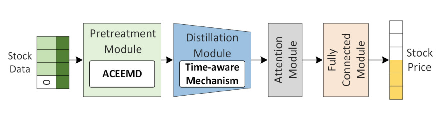
In this paper, a solution known as ACEFormer is proposed for predicting stock trends. ACEFormer leverages the power of ACEEMD, alongside a time-aware mechanism and an attention mechanism. The time-aware mechanism enhances the attention mechanism’s ability to accurately handle stock data.
In this part, the ACEFormer, a novel approach combining advanced techniques from both transformers and autoencoders, is explained. It aims to improve the efficiency and accuracy of language modeling tasks.
The algorithm ACEEMD, developed for reducing noise in the model, is introduced. Noise is a common issue that can impact the performance of language models. ACEEMD, which stands for Adaptive Contextual Embedded Energy Minimization Distillation, provides a solution to this problem by incorporating a distillation mechanism that separates relevant information from noisy inputs. This algorithm helps to enhance the quality of the learned representations by filtering out unnecessary noise.
The time-aware mechanism of ACEFormer is described next. Time-awareness is a crucial aspect in various natural language processing tasks, as the temporal order of words often carries important semantic information. The time-aware mechanism in ACEFormer is specifically designed to capture and encode temporal dependencies in the input data. It leverages self-attention mechanisms to effectively model and incorporate temporal information into the language modeling process. By considering the temporal context, ACEFormer is able to generate more accurate and contextually appropriate predictions.
The ACEFormer model is designed to predict future stock values using historical data. It consists of several components that work together to process the input data and extract relevant features.
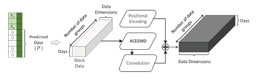
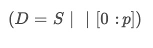
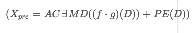
First, the pretreatment module prepares the input stock data for further processing. It uses a special algorithm to identify patterns in the data. Consider a set of stock data called S , where each element represents the price, trading volume, and two stock market indices for a specific day. To predict future values, unknown values are replaced with zeros, and a sequence of zeros is added to represent the days to be predicted. The resulting input data for the model is denoted as:
The pretreatment module applies algorithms called f and g to process the input data, and it incorporates positional encoding. The output of this module, denoted as
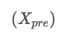
is calculated by passing the input data through the ACEEMD algorithm, which combines f and g, and adding positional encoding using the equation:
Next, the distillation module extracts the main features from the data. It uses probability self-attention to highlight important features and reduces the dimension of the feature data through convolution and pooling operations. Additionally, it incorporates a time-aware mechanism to enhance the weight of different positions, capturing important temporal patterns. This module helps reduce the number of parameters and focus on critical features.
The attention module follows the distillation module and further refines the feature representation, enhancing the accuracy of the predictions.
Finally, the fully connected module uses linear regression to produce the final predicted values. It takes the extracted features from the attention module and performs regression analysis to estimate future stock values.
x(t)
|
+-----------------+------------------+-------------------+
| | | |
pe1 = x(t) + E1(n[1]) ... pem = x(t) + E1(n[m])
| ... | |
pm1 = x(t) + E1(-n[1]) ... pmm = x(t) + E1(-n[m])
| ... | |
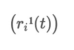
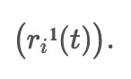
r1^1(t) = AM(pe1, pm1) ... rm^1(t) = AM(pem, pmm)
| ... | |
+-----------------+------------------+-------------------+
|
r1(t) = (1/m) * Σ r1^i(t) from i=1 to m
|
IMF1 = x(t) - r1(t)The ACEEMD algorithm, or Adaptive Complementary Ensemble Empirical Mode Decomposition, improves curve fitting in stock data by mitigating endpoint effects and preserving outliers. This is particularly important in the context of trading. Here is the structure of the ACEEMD algorithm, illustrated above.
The input data, representing the stock data and denoted as
, is processed by the ACEEMD algorithm. The algorithm introduces Gaussian noise,
to the input data. Generally, there are 5 sets of such noises
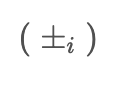
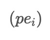
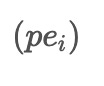
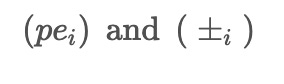
used in ACEEMD. These noises are combined with the input data to create two modified datasets, pe_i and pm_i, with opposite signs for the added noises.
The generating function,
, is then applied to remove the noise from the data. This step is the core part of ACEEMD. The resulting denoised data is represented by
, where I refers to the i-th set of Gaussian noise used.
Furthermore, the ACEEMD algorithm has two main improvements. First, to address endpoint effects, cubic interpolation is used in ACEEMD. The input data points for this interpolation are created using the endpoints and extreme points of the original data. The middle points, which are the data corresponding to the midpoint between the peaks and troughs, are also included to preserve short-term stock trends.
   BEGIN
     |
Input \( pe_i, pm_i \)
     |
     |
     v
Is \( pe_i \) IMF?
  /  \
 /    \
Yes    No
 |      |
 |     \( pe_i = pe_i - \frac{up(pe_i) + down(pe_i)}{2} \)
 |      |
 |     \( pm_i = pm_i - \frac{up(pm_i) + down(pm_i)}{2} \)
 |      |
 +------+
     |
     v
\( r_1^i(t) = \frac{(1 - \alpha) pe_i + \alpha pm_i}{2} \)
     |
    END
Secondly, in above chart it is presented the flowchart of the core function
of ACEEMD. The process begins with the input of
and
. If
is already an Intrinsic Mode Function (IMF), then the process stops. However, if pe_i is not an IMF, it is updated by subtracting the average of its upper and lower envelopes, and the same operation is performed on pm_i. This iterative process continues until pe_i becomes an IMF.
The denoised data
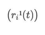
is obtained by calculating a weighted average of
and pm_i, with a default weight of 0.5. This process of obtaining denoised data is repeated iteratively with different sets of Gaussian noise, resulting in multiple denoised datasets
The first-order IMF component, denoted as
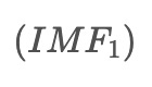
, is obtained by taking a weighted average of the intermediate signals between:
In the “Time-Aware Mechanism” section, a method used in a distillation module is discussed. This method employs linear regression and a bias to create a matrix that enhances the feature content and reduces information loss in the output features, thus improving the quality of the output.
The method utilizes two components: weights and a bias matrix. The weights, denoted as W_t, and the bias matrix, denoted as b_t, are used to calculate a matrix called T, which captures time-aware information. The mathematical calculation for obtaining this matrix is
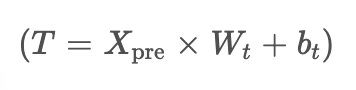
. Here,
represents the input data.
This time-aware mechanism operates on the same input data used for probability attention, effectively extracting features while ensuring no valuable information is lost. It optimizes the feature extraction process.
The output of the distillation module is denoted as \( D \). This output is expressed as
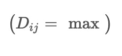
over a window of size 2, where the probability attention operator
is applied, and the time-aware mechanism matrix T is incorporated. This expression indicates taking the maximum value within a window, combining it with the attention operator and the time-aware mechanism matrix.
In this section, the datasets utilized to test the method are explained. Two real-world datasets, NASDAQ100 and SPY500, were chosen to assess the effectiveness of the approach. These datasets span over ten years and originate from the US stock markets. NASDAQ100 comprises 102 stocks from non-financial companies listed on the NASDAQ exchange, while SPY500 represents the Standard and Poor’s 500 index, tracking the performance of 500 large companies listed on different US stock exchanges.
For the experiments, data from January 3, 2012, to January 28, 2022, was selected. To ensure continuity, weekends and public holidays were removed from the dataset. After this data cleansing process, the dataset was divided into three distinct sets: a training set spanning from January 3, 2012, to June 25, 2021, a validation set covering the period from June 28, 2021, to September 7, 2021, and a testing set encompassing the timeframe from September 7, 2021, to January 28, 2022. Additionally, supplementary data from the Dow Jones Industrial Average (DJIA) and NASDAQ were incorporated as secondary sources in the experiments.
In the “Model Setting” section, the aim is to ensure that prediction results are not influenced by the random starting numbers used during training. To guarantee accuracy and reliability, a multi-step approach is adopted.
Firstly, the model is trained multiple times, specifically running it through five training cycles using the training data. By conducting the training process several times, the impact of random variation, which can potentially skew results, is mitigated. This approach captures a range of potential outcomes and decreases the likelihood of results being influenced by chance fluctuations.
After completing the five training runs, the performance of each model is evaluated using validation data. The models are assessed based on their ability to accurately predict the outcomes of the validation data. This evaluation provides a quantitative measure to determine the effectiveness of each model in capturing the underlying patterns in the data.
Following the evaluation, the model that demonstrates the best performance on the validation test is selected. This model, which proves to be the most adept at capturing patterns and making accurate predictions, becomes the top-performing model.
To ensure the consistency of predictions, this top-performing model is used to forecast outcomes on the test data. By utilizing the best-performing model, potential variability caused by randomness and other confounding factors is accounted for and reduced.
As the performance of the forecasting models is evaluated, two specific metrics are used: Accuracy and the Matthews Correlation Coefficient. Accuracy is measured on a scale from 0 to 100, with higher values indicating better performance. The Matthews Correlation Coefficient (MCC) ranges from -1 to 1, also measuring how well the models predict trends, with higher values indicating better performance.
