

Analyzing Pairs Trading Strategy with Coca-Cola and PepsiCo Stocks
A Statistical Arbitrage Approach Using Python for Comparative Performance Analysis with Buy & Hold Strategy

Pairs trading is a market-neutral strategy that capitalizes on the correlation of price movements between two assets. The purpose of this article is to examine a pairs trading strategy using Coca-Cola (KO) and PepsiCo (PEP) stocks. Both Coca-Cola and PepsiCo operate in the soft beverage industry, despite differences in their financial fundamentals, including Coca-Cola’s higher net income compared to PepsiCo’s larger sales, and their stock prices tend to move in the same direction when industry-wide events, such as new regulations, affect them.
A Python-based approach will be used in this article to implement a pairs trading strategy, analyzing the price movements of KO and PEP to identify profitable trading opportunities when their prices diverge from their historical relationship. By comparing statistical arbitrage to a traditional 50/50 buy-and-hold approach, we provide insight into the potential benefits and challenges associated with statistical arbitrage.
Notebook at the end of this article!
# python 3.7

# For yahoo finance
import io
import re
import requests

# The usual suspects
import numpy             as np
import pandas            as pd
import matplotlib.pyplot as plt

# Fancy graphics
plt.style.use('seaborn')

# Getting Yahoo finance data
def getdata(tickers,start,end,frequency):
    OHLC = {}
    cookie = ''
    crumb = ''
    res = requests.get('https://finance.yahoo.com/quote/SPY/history')
    cookie = res.cookies['B']
    pattern = re.compile('.*"CrumbStore":\{"crumb":"(?P<crumb>[^"]+)"\}')
    for line in res.text.splitlines():
        m = pattern.match(line)
        if m is not None:
            crumb = m.groupdict()['crumb']
    for ticker in tickers:
        url_str = "https://query1.finance.yahoo.com/v7/finance/download/%s"
        url_str += "?period1=%s&period2=%s&interval=%s&events=history&crumb=%s"
        url = url_str % (ticker, start, end, frequency, crumb)
        res = requests.get(url, cookies={'B': cookie}).text
        OHLC[ticker] = pd.read_csv(io.StringIO(res), index_col=0,
                                   error_bad_lines=False).replace('null', np.nan).dropna()
        OHLC[ticker].index = pd.to_datetime(OHLC[ticker].index)
        OHLC[ticker] = OHLC[ticker].apply(pd.to_numeric)
    return OHLC

# Assets under consideration
tickers = ['PEP','KO']

data = None
while data is None:
    try:
        data = getdata(tickers,'946685000','1687427200','1d')
    except:
         pass

KO = data['KO']
PEP = data['PEP']
The purpose of this code is to achieve the task of retrieving historical stock price information from Yahoo Finance using their API for specified tickers. For data manipulation and visualization, Numpy, Pandas, Matplotlib, and other libraries are imported into the program.
The main function, getdata, is a function that accepts a list of stock symbols, a start and end date, and a frequency of data availability. During the execution of the script, it creates a dictionary in which it stores the Open-High-Low-Close (OHLC) data for each ticker. In order to make API requests, the function first requests the history page of Yahoo Finance for obtaining a cookie and a crumb.
There is a function in the function, which constructs a URL from which historical data can be downloaded for each ticker, sends a GET request to the URL, and reads the response into a pandas DataFrame. In this process, it replaces all null values with NaNs and removes any missing entries in order to clean up the data. There is a conversion of the date index to a datetime format, and all of the values are changed to numeric types.
In the code, an array of tickers is initialized, for example, PEP and KO, and and the data is requested repeatedly until the data is successfully fetched. If the data dictionary is returned, then it extracts the DataFrames for KO and PEP from it, allowing easy access and analysis of the stock data in the returned DataFrames.
#tc = -0.0005 # Transaction costs

pairs = pd.DataFrame({'TPEP':PEP['Close'].shift(1)/PEP['Close'].shift(2)-1,
                      'TKO':KO['Close'].shift(1)/KO['Close'].shift(2)-1})

# Criteria to select which asset we're gonna buy, in this case, the one that had the lowest return yesterday
pairs['Target'] = pairs.min(axis=1)

# Signal that triggers the purchase of the asset
pairs['Correlation'] = ((PEP['Close'].shift(1)/PEP['Close'].shift(20)-1).rolling(window=9)
                        .corr((KO['Close'].shift(1)/KO['Close'].shift(20)-1)))

Signal = pairs['Correlation'] < 0.9

# We're holding positions that weren't profitable yesterday
HoldingYesterdayPosition = ((pairs['Target'].shift(1).isin(pairs['TPEP']) &
                             (PEP['Close'].shift(1)/PEP['Open'].shift(1)-1 < 0)) |
                            (pairs['Target'].shift(1).isin(pairs['TKO']) &
                             (KO['Close'].shift(1)/KO['Open'].shift(1)-1 < 0))) # if tc, add here

# Since we aren't using leverage, we can't enter on a new position if
# we entered on a position yesterday (and if it wasn't profitable)
NoMoney = Signal.shift(1) & HoldingYesterdayPosition

pairs['PEP'] = np.where(NoMoney,
                        np.nan,
                        np.where(PEP['Close']/PEP['Open']-1 < 0,
                                 PEP['Close'].shift(-1)/PEP['Open']-1,
                                 PEP['Close']/PEP['Open']-1))

pairs['KO'] = np.where(NoMoney,
                       np.nan,
                       np.where(KO['Close']/KO['Open']-1 < 0,
                                KO['Close'].shift(-1)/KO['Open']-1,
                                KO['Close']/KO['Open']-1))

pairs['Returns'] = np.where(Signal,
                            np.where(pairs['Target'].isin(pairs['TPEP']),
                                      pairs['PEP'],
                                      pairs['KO']),
                             np.nan) # if tc, add here

pairs['CumulativeReturn'] = pairs['Returns'].dropna().cumsum()
With the use of pandas for data manipulation, this code is used to analyze and trade two stocks as part of a statistical arbitrage strategy using pandas for data analysis. There is a formula in this function that calculates the daily returns for the stocks PEP and KO by comparing their closing prices from the previous two days. These returns are then stored in a DataFrame called pairs. Upon identifying the stock that had the lowest return from the previous day, the Target column is used to record which stock had the lowest return.
A rolling window of nine days is then used to calculate the correlation between the returns of the stocks in an attempt to evaluate their recent behavior. When the correlation of the two variables falls below a threshold of 0.9, a purchase signal is generated. The HoldingYesterdayPosition variable provides information about whether there are any unprofitable positions that were held yesterday. The NoMoney variable is used to prevent new entries from being made if a purchase signal exists, but there is already an unprofitable position present.
After this, the code determines how much return each stock will have based on the NoMoney condition for each stock. A return will be assigned to NaN if there is no money available; otherwise, the return will be checked today’s return, and if the return today’s is negative, the return for tomorrow’s will be used. Using the Target stock as the basis for the calculation of returns, the overall returns are calculated, and they can be seen in the Returns column.
It is also important to note that the code calculates cumulative returns over time for executed trades, providing a running total in the CumulativeReturn column of profits or losses in order to evaluate the trading strategy’s performance over time.
# Pepsi returns
ReturnPEP = PEP['Close']/PEP['Open']-1
BuyHoldPEP = PEP['Adj Close']/float(PEP['Adj Close'][:1])-1

# Coca Cola returns
ReturnKO = KO['Close']/KO['Open']-1
BuyHoldKO = KO['Adj Close']/float(KO['Adj Close'][:1])-1

# Benchmark
ReturnBoth = (ReturnPEP+ReturnKO)/2
BuyHoldBoth = ((BuyHoldPEP+BuyHoldKO)/2).fillna(method='ffill')
A code that calculates the return on Pepsi stock and Coca-Cola stock over a specified period of time is provided below. Firstly, it determines the daily return for each stock by comparing the current closing price with the previous day’s opening price. The result is then expressed as a percentage change between the two prices. As a measure of whether a stock is likely to achieve a buy-and-hold return, the percentage change between the adjusted closing price on the first day and the current adjusted closing price is used to calculate the buy-and-hold return. Last but not least, the code calculates an average of the daily returns of both stocks to create a benchmark return and it computes an average of the buy-and-hold returns with forward filling in place of any missing data points in order to ensure a complete time series of returns.
returns = pairs['Returns'].dropna()
cumulret = pairs['CumulativeReturn'].dropna()

fig, ax = plt.subplots(figsize=(16,6))

hist1, bins1 = np.histogram(ReturnBoth.dropna(), bins=50)
width = 0.7 * (bins1[1] - bins1[0])
center = (bins1[:-1] + bins1[1:]) / 2

ax.bar(center, hist1, align='center', width=width, label='50/50 Returns')

hist2, bins2 = np.histogram(returns, bins=50)
ax.bar(center, hist2, align='center', width=width, label='Pairs Trading')

plt.legend()
plt.show()

print('=====Strategy Returns=====')
print('Mean return =',round((returns.mean())*100,2),"%")
print('Standard deviaton =',round((returns.std())*100,2),"%")
print("==========================")
print('Worst return =',round((min(returns))*100,2),"%")
print('Best return =',round((max(returns))*100,2),"%")
print("=========================")
print('Lower quantile =',round((returns.quantile(q=0.25))*100,2),"%")
print('Median return =',round((returns.quantile(q=0.5))*100,2),"%")
print('Upper quantile =',round((returns.quantile(q=0.75))*100,2),"%")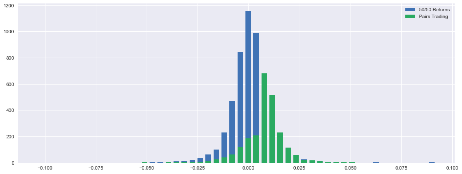
An analysis of the returns that can be expected from a pairs trading strategy when compared to a 50/50 return setup is presented in this code. This function extracts Returns and CumulativeReturn columns from a DataFrame named pair and ensures that any missing values are removed to ensure that the results are as clear as possible.
It is created a histogram showing the distribution of returns within 50 bins with a bar width adjusted for a more accurate representation of the distribution. The first histogram displays the 50/50 returns, while the second shows the pairs trading returns, both plotted on the same axes for ease of comparison.
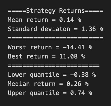
After viewing the visualization, the code calculates various statistics for the pairs trading returns, such as the mean, standard deviation, the worst and best returns, and the lower, median, and upper quartiles based on the visualization. The values are rounded to two decimal places and shown as percentages, allowing a clear understanding of how the strategy performed over time.
# Some stats, this could be improved by trying to estimate a yearly sharpe, among many others
executionrate = len(returns)/len(ReturnBoth)

maxdd = round(max(np.maximum.accumulate(cumulret)-cumulret)*100,2)

mask = returns<0
diffs = np.diff(mask.astype(int))
start_mask = np.append(True,diffs==1)
mask1 = mask & ~(start_mask & np.append(diffs==-1,True))
id = (start_mask & mask1).cumsum()
out = np.bincount(id[mask1]-1,returns[mask1])
badd = round(max(-out)*100,2)

spositive = returns[returns > 0]
snegative = -returns[returns < 0]
winrate = round((len(spositive)/(len(spositive)+len(snegative)))*100,2)

beta = round(returns.corr(ReturnBoth),2)

sharpe = round((float(cumulret[-1:]))/cumulret.std(),2)

tret = round((float(cumulret[-1:]))*100,2)
A code snippet that calculates various metrics related to investment returns, focusing on risk and performance, is shown below. The execution rate is determined by comparing the length of the returns array with another array named ReturnBoth, which provides insight into the number of trades that have been executed, based on the ratio between the length of the returns array and the ReturnBoth array. It then calculates a maximum drawdown that represents the largest drop from a peak to a trough in cumulative returns, expressed as a percentage, by comparing cumulative returns against their maximum value in order to find the maximum difference between it and a peak.
As a result of the code being written to identify periods of negative returns, a mask is created to track these occurrences and a filter is applied to filter out the brief negative periods that follow positive periods. Badd, which is the maximum percentage of drawdown caused by negative returns, is calculated by counting the contribution of negative returns. Using both positive and negative returns as the basis for measuring the success of an investment strategy, the win rate is calculated as the percentage of positive returns relative to the total number of returns in the strategy.
It is also calculated by the correlation between beta and ReturnBoth in order to reflect the volatility of returns as compared to ReturnBoth. In order to calculate the Sharpe ratio, we must take into account the cumulative returns and the standard deviation of those returns, which indicate the average return above the risk-free rate for a unit of volatility. Lastly, tret is calculated as the last cumulative percentage of return, which represents the amount of return achieved by an investment over a period of time.
plt.figure(figsize=(16,6))
plt.plot(BuyHoldBoth*100, label='Buy & Hold 50/50')
plt.plot(cumulret*100, label='Pairs Trading', color='coral')
plt.xlabel('Time')
plt.ylabel('Returns (in %)')
plt.margins(x=0.005,y=0.02)
plt.axhline(y=0, xmin=0, xmax=1, linestyle='--', color='k')
plt.legend()
plt.show()

print("Cumulative Return = ",tret,"%")
print("=========================")
print("Execution Rate = ",round(executionrate*100,2),"%")
print("Win Rate = ",winrate,"%")
print("=========================")
print("Maximum Loss = ",maxdd,"%")
print("Maximum Consecutive Loss = ",badd,"%")
print("=========================")
print("Beta = ",beta)
print("Sharpe = ",sharpe)
# Return ("alpha") decay is pretty noticeable from 2011 onwards, most likely due to overfitting, they're not reinvested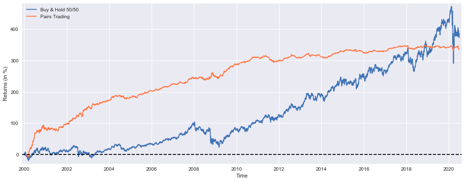
A plot was created by using the Matplotlib library in order to compare two investment strategies: Buy & Hold 50/50 and Pairs Trading in this code. A figure with a defined size is set up and the cumulative returns of both strategies are plotted on the plot, with the returns scaled to represent the percentage return on each strategy. This graph is displayed with the x-axis labeled Time, and the y-axis labeled Returned in percent, with adjusted margins for a better visual spacing. As a reference point, an arrow with dashed lines is drawn at the y=0 level.
On the final visualization, a legend distinguishes between the two plotted lines, and the final visualization can be viewed. Aside from printing several performance metrics to the console, the code also prints several metrics about the performance of the system, including cumulative return, execution rate, win rate, maximum loss, maximum consecutive loss, beta, and Sharpe ratio. As a result of this summary, we are able to evaluate the effectiveness and risk metrics associated with these strategies, while noting that the decline in returns since 2011 may be attributed to overfitting and the failure to reinvest the returns.
BuyHoldBothYTD = (((PEP['Adj Close'][-252:]/float(PEP['Adj Close'][-252])-1)+(KO['Adj Close'][-252:]/float(KO['Adj Close'][-252])-1))/2).fillna(method='ffill')
StrategyYTD = returns[-92:].cumsum()

plt.figure(figsize=(16,6))
plt.plot(BuyHoldBothYTD*100, label='Buy & Hold 50/50')
plt.plot(StrategyYTD*100, label='Pairs Trading', color='coral')
plt.xlabel('Time')
plt.ylabel('Returns (in %)')
plt.margins(x=0.005,y=0.02)
plt.axhline(y=0, xmin=0, xmax=1, linestyle='--', color='k')
plt.legend()
plt.show()

print('Buy & Hold 50/50 YTD Performance (at 1 July 2020) =',round(float(BuyHoldBothYTD[-1:]*100),1),'%')
print('Strategy YTD Performance =',round(float(StrategyYTD[-1:]*100),1),'%')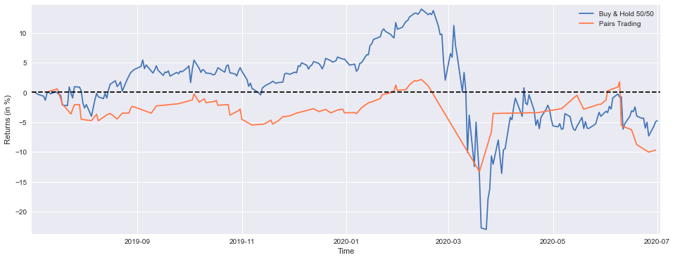
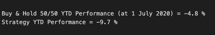
In this code, we calculate and visualize the year-to-date performance of two investment strategies based on an equal allocation to PepsiCo and Coca-Cola, as well as a Pairs Trading strategy, in comparison with the Buy and Hold strategy. It is important to keep in mind that a Buy and Hold strategy uses adjusted closing prices for both stocks over a period of 252 trading days in order to calculate their returns relative to their initial values, averaging them and filling in any gaps with forward fill in case of missing values. Over the past 92 trading days, cumulative returns have been calculated from a returns variable for the Pairs Trading strategy that was used to calculate the returns. In the plotting section, the performance of both strategies over time is shown as percentage returns, with properly labeled axes and a reference line at zero. There is a legend defining the two strategies, and the final performance metrics, rounded to one decimal place, show how the two strategies performed on July 1, 2020 in terms of how they performed in terms of their performance.
