

Basic Regression With Tensorflow and Keras
Basic Regression With Tensorflow and Keras
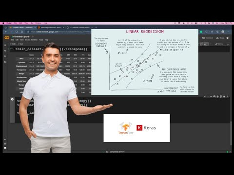
In this post, i'll show you the basic of regression with single variable linear regression and multiple variable linear regression.

In a regression problem, the aim is to predict the output of a constant value, like a price or a probability. Contrast this with a classification problem, where the objective is to select a class from a list of classes (for example, where a picture contains an apple or an orange, recognising which fruit is in the picture).
This tutorial uses the classic Auto MPG dataset and demonstrates how to build models to predict the fuel efficiency of the late-1970s and early 1980s automobiles. To do this, you will provide the models with a description of many automobiles from that time period. This description includes attributes like cylinders, displacement, horsepower, and weight.
import matplotlib.pyplot as plt
import numpy as np
import pandas as pd
import seaborn as sns

# Make NumPy printouts easier to read.
np.set_printoptions(precision=3, suppress=True)
import tensorflow as tf
from tensorflow import keras
from tensorflow.keras import layers
print(tf.__version__)Get the data
First, download and import the dataset using pandas:
url = 'http://archive.ics.uci.edu/ml/machine-learning-databases/auto-mpg/auto-mpg.data'
column_names = ['MPG', 'Cylinders', 'Displacement', 'Horsepower', 'Weight',
                'Acceleration', 'Model Year', 'Origin']

raw_dataset = pd.read_csv(url, names=column_names,
                          na_values='?', comment='\t',
                          sep=' ', skipinitialspace=True)
dataset = raw_dataset.copy()
dataset.tail()Watch Video
If you don’t want to read, you can watch the video.
Clean the data
The dataset contains a few unknown values:
dataset.isna().sum()Drop those rows to keep this initial tutorial simple:
dataset = dataset.dropna()The "Origin" the column is categorical, not numeric. So the next step is to one-hot encode the values in the column with pd.get_dummies.
dataset['Origin'] = dataset['Origin'].map({1: 'USA', 2: 'Europe', 3: 'Japan'})dataset = pd.get_dummies(dataset, columns=['Origin'], prefix='', prefix_sep='')
dataset.tail()Split the data into training and test sets
Now, split the dataset into a training set and a test set. You will use the test set in the final evaluation of your models.
train_dataset = dataset.sample(frac=0.8, random_state=0) test_dataset = dataset.drop(train_dataset.index)Inspect the data
Review the joint distribution of a few pairs of columns from the training set.
The top row suggests that the fuel efficiency (MPG) is a function of all the other parameters. The other rows indicate they are functions of each other.
sns.pairplot(train_dataset[['MPG', 'Cylinders', 'Displacement', 'Weight']], diag_kind='kde')<seaborn.axisgrid.PairGrid at 0x7f3f8ac88b50>
Let’s also check the overall statistics. Note how each feature covers a very different range:
train_dataset.describe().transpose()Split features from labels
The rest of the article is available for subscribers please subscribe to my newsletter. By subscribing you get access to hundreds of source code, written explanations, and tutorial series just like this. You can unlock the entire TensorFlow series and all of the tutorials.