Beyond the Model: The Hard Truths of Deploying ML in Production

Why Algorithms Are Not Enough: A Guide to the ML Pipeline

Nov 28, 2025

∙ Paid

This is only the first chapter. To access the complete book, download the full PDF using the button provided at the end of this article.

$\mathbb{U} \int \varepsilon \quad \left[ \frac{ \tau \hbar e }{ \beta \cup \tau \tau \odot \eta } \right]_{\mathbf{b} \epsilon \ell \odot \omega} $

Building a successful ML product begins by recognizing that the model is only one piece of a larger machine. An effective system splits into distinct layers — Interface, Data, ML algorithms, Infrastructure, and Hardware — each with a clear responsibility: Data collects, stores, preprocesses, and labels inputs; ML algorithms handle model selection, training, and inference; Infrastructure implements pipelines, deployment, serving, and operationalization; Hardware supplies compute for both training and inference; and the Interface mediates user interactions and consumes model outputs. This decomposition matters because correctness and performance flow downhill: poor data compromises model quality, inadequate infrastructure limits throughput and latency, and mismatched hardware makes even the best model impractically slow or expensive.

Because ML research continually produces new algorithms, system design must treat the algorithm layer as replaceable rather than central. An algorithm-agnostic design provides stable interfaces and repeatable processes so teams can swap or upgrade models without rearchitecting the whole system. That mindset also shapes the question of whether to use ML at all: the decision boundary — when and when not to use machine learning — is a cost‑benefit judgment based on problem suitability, data availability, operational complexity, and deployment constraints. When ML is appropriate, the emphasis shifts from prescribing a single technique to following a model selection process that reliably evaluates options in the context of system constraints (see Chapter 5). In practice that means measuring not only research metrics but also production considerations such as latency during serving, memory and compute footprints on target Hardware, and how easy it is to deploy and version a candidate.

At production scale, two realities drive architecture and operations. First, ML systems typically consume massive amounts of data and need heavy computational power, which creates bottlenecks in storage capacity, network I/O, training throughput, and inference latency; these constraints force trade-offs in data retention, batching, and model complexity. Second, production ML requires engineering practices that go beyond research: monitoring, validation, maintainability, rollback procedures, and automated retraining become essential to handle data quality issues, model drift, and hardware limits. This engineering posture also responds to non‑technical stakes — unaddressed deployment issues can cause serious societal harm or business failure — so safety, fairness, and compliance must be treated as first‑class system requirements. Teams frequently face a time‑to‑market vs. robustness trade‑off: shipping fast can expose users and business to risk, while delaying until every operational edge case is covered increases time and cost. As a result, practical ML systems are iteratively engineered to be deployable, reliable, scalable, and adaptable, with continuous loops for monitoring, retraining, versioning, and rollback to manage implicit failure modes and maintain long‑term correctness.

When to Use Machine Learning

Machine learning is a tool, not a silver bullet — the first question for any project is whether its benefits outweigh the costs. Ask explicitly is ML necessary or cost-effective? before proceeding: ML can deliver value when hand-coded rules fail, but it also introduces development, data, and maintenance overhead that must factor into your return‑on‑investment calculation. Framing ML correctly helps you make that judgment. At its core, Machine Learning (ML) can be decomposed into six meaningful pieces — learn, complex, patterns, existing data, predictions, and unseen data — and each term imposes an operational requirement on how you approach the problem.

Start with what “learn” and “complex” imply: learn means using inductive approaches that derive behavior from examples rather than explicit rules, so you must supply representative examples instead of coding logic by hand and expect model behavior to emerge from training. Complex signals that the relationships you care about are hard to enumerate — they may be nonlinear, high‑dimensional, or combinatorial — and therefore impractical to capture with deterministic code or simple heuristics. “Patterns” refers to statistical regularities rather than immutable laws, so what the model exploits are correlations that can be useful but also spurious; as a result you must validate findings and test for robustness. Taken together, these ideas explain why ML is chosen for problems where domain logic is messy or too large to express as rules, and why emergent behavior and careful validation are part of the price you pay.

The remaining terms tie ML to data and decisioning. Existing data is a gating constraint: effective ML demands sufficient volume, accurate labels, coverage of relevant cases, and representativeness of future inputs. Predictions reminds us that model outputs are typically probabilistic and approximate, so you need clear metrics, calibration, and an analysis of how much downstream error your system can tolerate. Finally, unseen data makes generalization the central engineering objective and risk: you must plan for dataset bias, distribution shift, and out‑of‑distribution cases, and implement monitoring and robustness checks in production. These requirements drive concrete operational costs — data collection and labeling, training compute, model validation, ongoing drift monitoring, and retraining — and they explain the trade‑off: prefer non‑ML solutions when rules or algorithms are simpler, cheaper, more predictable, or when data is scarce, because ML buys flexibility and pattern discovery at the cost of explainability, repeatability, and higher maintenance overhead.

In practice, use ML when four conditions hold together: the problem is driven by complex patterns that are impractical to hand‑code, you have adequate and representative historical data, you can define measurable labels or objectives for evaluation, and the system can tolerate approximate, probabilistic predictions. If one of these elements is missing — for example, insufficient data or a requirement for deterministic, fully explainable decisions — a rule‑based approach will often be the better, cheaper choice. Ultimately, adopting ML is a strategic decision: it can unlock solutions that hand‑written logic cannot capture, but it requires accepting emergent behavior, investing in data and operational processes, and planning for ongoing validation and maintenance.

Relational systems and machine learning solve different classes of problems, and understanding that distinction explains why ML matters. A relational database is deterministic and rule-based: you declare an explicit schema and relationships, and the system returns results that follow those rules. Machine learning, by contrast, provides an inductive mechanism that infers patterns from examples rather than being told exact relationships. To do that you must give the learner a training signal — typically a dataset of inputs paired with desired outputs — so the system can approximate a mapping f: X → Y. In the common supervised learning pattern you supply many (input, output) pairs; during training the model adjusts parameters to minimize a loss between its predictions and the true labels, producing a predictor that generalizes to unseen inputs. For example, in an Airbnb price-prediction model the inputs (features) might include square footage, room count, neighborhood, amenities, and rating, while the label is the rental price; by engineering useful features and choosing the right label, the model learns to estimate price for new listings.

Putting learning into production requires clearly defined components and a left-to-right data flow during training that collapses into a single step at inference time. First you perform data collection and labeling to create the training set; next you perform feature representation/engineering to map raw attributes into the model’s inputs. The learning algorithm/model acts as a function approximator and is trained inside a training loop that uses a loss, an optimizer, and validation to guide parameter updates. Once trained, inference serving applies only the trained model to new inputs. This separation explains performance characteristics and costs: training is typically compute- and time-intensive — often requiring batch or iterative optimization and distributed compute to scale — whereas inference is usually optimized for low latency and high throughput through model size choices, hardware acceleration, and batching.

Designing an effective ML system is an exercise in managing trade-offs around capacity, data, and robustness. Model capacity determines how complex a relationship the model can represent: too much capacity risks overfitting to training data, while too little leads to underfitting; inductive bias (architecture and regularization choices) guides generalization when data is limited. The system’s ability to learn also depends on sample complexity — the volume, diversity, and label fidelity of training data — because insufficient, biased, or noisy labels produce systematic errors. Common failure modes include overfitting, underfitting, label noise, and covariate shift (distribution drift that degrades runtime performance). As a result you need validation and testing, regularization, monitoring for drift, retraining pipelines, and robust feature selection to build resilience. Finally, practical design knobs — feature choices, label definition, model architecture, loss function, regularization, and hyperparameters — directly influence generalization, latency, and robustness; in many cases collecting better labeled data or changing model bias yields bigger gains than micro-optimizing algorithms. The key takeaway is that learning systems are built around data plus inductive machinery: get the training signal and representation right, and you enable generalization; ignore data quality or capacity trade-offs, and the system will reliably expose its failure modes.

Complex: the patterns are complex

Thanks for reading! This post is public so feel free to share it.

When you design a component that maps inputs to outputs, the first and most important decision is a problem class distinction: is the behavior expressible as an explicit, finite mapping or is it better modeled as a high‑dimensional, implicitly defined function? This matters because the answer determines everything that follows — from the architecture and operational cost to how you diagnose failures. A canonical explicit example is zip code → state, where a fixed, known list of key→value pairs exactly defines the behavior. In contrast, estimating a rental price from many listing characteristics is a high‑dimensional problem: the relationship emerges from data, is nonlinear, and is impractical to enumerate by hand.

When to Use Machine Learning

Complex: the patterns are complex

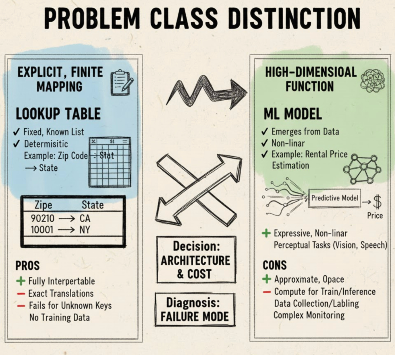
For the explicit case you use lookup tables: store a canonical mapping, retrieve the value deterministically for a given key, and maintain the table entries as the single source of truth. Implementation responsibilities are straightforward — reliable storage, fast retrieval (constant time), and operational processes to update or correct entries — and they require no labeled examples or model training. As a result you get fully interpretable, exact translations with very low latency. The obvious limitation is coverage: a lookup simply fails or returns unknown for keys not present in the table, and its expressiveness is bounded by the encoded keys. Prefer this approach when the mapping is explicit, finite, and stable.

When the mapping is complex or emergent, you use ML models and a data‑driven learning pattern: collect features and target labels, train a model to approximate the underlying mapping, and serve it for inference. Component responsibilities expand to include data collection and labeling, model training, deployment/serving infrastructure, and lifecycle activities such as retraining and versioning. This pipeline translates observed examples into learned parameters that produce predictions. The trade‑offs are clear: ML is expressive and can capture nonlinear, high‑dimensional patterns (which is why it succeeds on perceptual tasks like object detection and speech recognition), but models are approximate, often opaque, and require compute for both training and inference. Performance and latency depend on model complexity and serving infrastructure, and engineering cost rises because you must provision compute, collect labeled data, and continuously monitor model behavior.

These two patterns also differ in how you diagnose errors and in the decision rules you apply. A lookup error points you at table coverage or stale data — you fix the table. A model error points you at dataset bias, insufficient examples, or model capacity — you analyze data and training. Operationally, that means different monitoring, alerting, and maintenance practices. In practice, choose the simplest component that satisfies your requirements: use rule/table‑based components for exact, finite mappings; invest in ML when the mapping is high‑dimensional, hard to formalize, or clearly emergent from data. The consequence of this choice shapes interpretability, latency, engineering effort, and the types of failure modes you must prepare to handle.

Patterns: there are patterns to learn

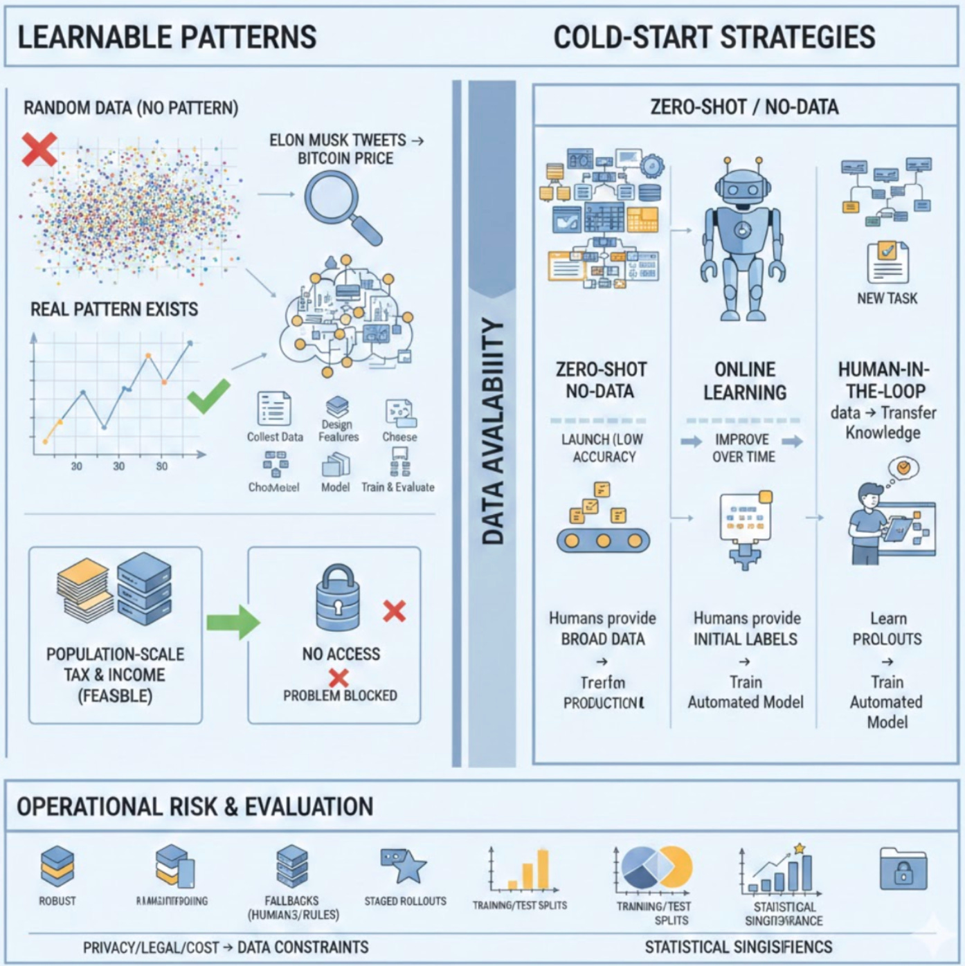
Machine learning only pays off when real, learnable patterns exist in the data. If the process you’re trying to model is effectively random — think of repeated outcomes from a fair die — there is no predictable signal for an ML algorithm to extract, so investing in models is wasteful. In practice, however, the existence of a pattern is often non-obvious and conditional: a relationship like “Elon Musk tweets → Bitcoin price moves” may be real, but it becomes detectable only after you collect the right observations, design informative features, choose a model with sufficient capacity, and apply rigorous training and evaluation. Because of this conditionality, a trained model’s inability to predict a target does not prove there is no underlying pattern; negative results can equally reflect limited dataset size, poor feature representation, an inappropriate model class, label noise, or sloppy evaluation.

A more practical hinge of whether ML is possible is data availability: supervised learning requires relevant input–output pairs at adequate scale and coverage. For example, predicting tax liabilities is theoretically possible only if you can access population-scale tax and income records — without that data, the problem is blocked irrespective of any underlying signal. Relatedly, techniques that look like they need “no data” have hidden dependencies: zero-shot (aka zero-data) performance on a new task succeeds not because the model learned from nothing, but because it was pre-trained on broad or related datasets and can transfer that prior knowledge. In contrast, online learning lets you deploy a model without task-specific pre-training by learning from production data over time; this removes the pre-training requirement at launch but trades it for poor initial performance and a risk of degraded customer experience while the model accumulates data. A common pragmatic middle ground is the human-in-the-loop bootstrap — “fake-it-til-you-make-it” — where humans provide initial predictions to generate labeled examples for later automated training; this accelerates getting a working service but slows scale-up, can introduce human label biases, and delays the payoff of full automation.

Because each cold-start option has different costs and failure modes, the choice among zero-shot, online learning, and human-in-the-loop depends on data availability, time-to-market, acceptable initial accuracy, and risk tolerance for user-facing errors — there is no universally optimal path. You must also address operational risk: putting insufficiently trained models into production causes immediate user-facing failures, loss of trust, and business harm. Mitigations include robust monitoring, fallbacks to human responders or rule-based logic, and staged rollouts that limit exposure while you validate performance. Finally, detecting whether a genuine pattern exists requires rigorous empirical practice: sound training/test splits, statistical-significance checks, and iterative experiments that isolate data, feature, and model factors. Data-collection constraints—privacy, legal access, or labeling cost—directly shape which patterns are feasible to learn; if you cannot acquire the necessary inputs (for example, private tax records), no amount of modeling will recover the signal. In short: verify pattern plausibility, confirm data availability, pick a cold-start strategy that matches your tolerance for initial errors, and instrument strong evaluation and operational guardrails before betting on ML.

Predictions: it’s a predictive problem

Machine learning works by estimating values rather than computing exact proofs: treat each task as “estimate the value of X” — whether X is a future outcome, a current hidden state, or the result of an expensive subroutine. This perspective matters because many engineering problems today are dominated by compute‑intensive subroutines (simulations, ray tracers, numerical solvers) that are costly to run repeatedly. By reframing such tasks as prediction problems you can train a model to act as a predictive estimator that approximates the expensive computation, turning a deterministic computation into a learned surrogate that produces answers far more cheaply at inference time.

That reframing yields a surrogate/emulator architecture: you replace an expensive exact computation with an ML model that maps inputs to approximate outputs. The economic benefit is amortized cost — you pay a large upfront training bill, but then enjoy many cheap, low‑latency inferences. As a result, systems that require many repeated queries see dramatic throughput gains per unit of compute, at the cost of accepting approximation error. A concrete example is graphics and rendering: models can approximate pixel‑level operations (image denoising, screen‑space shading) to deliver perceptually similar images with far less compute than running the full pipeline for every frame. Whether you choose this path depends on the core trade‑off of accuracy vs. compute/time: ML reduces latency and cost but introduces approximation error; acceptability hinges on the domain’s error tolerance and the downstream impact of mistakes.

Making a surrogate work in practice depends heavily on data and engineering choices. Surrogates require ground truth from the exact computation or labeled examples, so model generalization is bounded by the coverage and representativeness of the training set. Per‑query performance is constrained by inference latency, model size, and memory bandwidth, so the largest wins arise when the original exact computation dominates overall cost. Key configuration levers — model capacity and architecture, training dataset size and diversity, the loss/objective (L2 versus perceptual losses), and deployment latency/throughput targets — directly shape accuracy, speed, and robustness. You can scale by parallelizing inference and applying model quantization and serving optimizations, but you remain limited by inference compute, memory, and the model’s tendency to degrade under distributional shift; this creates operational needs for retraining and continual learning.

Those limitations produce important failure modes and system implications you must address. Surrogates can introduce systematic approximation bias, suffer catastrophic errors on out‑of‑distribution inputs, and have unbounded worst‑case deviations from the exact solution. This leads to a design pattern for resiliency: build hybrid pipelines that pair ML predictions with cheap validation checks or conditional fallbacks to the exact computation so critical or ambiguous cases are contained. Practically, adopting predictive approximations raises operational complexity — you need dataset generation pipelines, model evaluation metrics that include worst‑case analyses, monitoring and uncertainty estimation, and processes for incremental retraining and rollbacks. In short, use ML approximations when the cost of exact computation far exceeds acceptable approximation error and you have sufficient labeled data; otherwise prefer deterministic algorithms when correctness is required.

Unseen data: Unseen data shares patterns with the training data

Machine learning models work by extracting statistical regularities from historical data and using those regularities to make predictions about new cases. This becomes a problem whenever the new, unseen data does not share those same regularities — for example, training a model on app-download patterns from 2008 when the market was dominated by Koi Pond and then expecting it to predict downloads in 2020 is likely to fail because the underlying landscape has changed. Formally, the core requirement is that the training distribution and the distribution that generates unseen (test or production) data should be similar; saying two datasets are drawn from “similar probability distributions” is the precise way to express the alignment you need for learned patterns to remain useful.

A fundamental difficulty arises because the true distribution of future data is unknown a priori, so you can never be certain that the relationships your model learns will persist in deployment. To bridge that gap practitioners commonly make an explicit modeling assumption of temporal stability (users’ behaviors tomorrow ≈ users’ behaviors today). This assumption simplifies model design: if you accept it, you can train once on recent historical data and deploy standard ML pipelines that exploit recurring patterns. As a result you often get fast, low-cost wins in engineering time and immediate model performance, but you also increase fragility — if the world shifts, those same models can degrade quickly.

That fragility is the concrete failure mode known as distributional shift or temporal shift: when the data-generating process changes (different popular apps, new user behaviors), the statistical features the model relied on become irrelevant and performance drops. Because most ML algorithms today learn by exploiting recurring regularities, they excel on stable problems but perform poorly when those regularities disappear. To reduce this risk, your training data should be recent and representative of expected production conditions; stale historical examples bias models toward obsolete patterns. Equally important, practical systems must include detection and feedback: monitoring production performance, triggering investigation when metrics fall, and scheduling retraining or other corrective actions — in short, you cannot rely on “we’ll find out soon enough” without instrumentation that tells you when the assumption has broken.

Designing around this reality forces a trade-off. You can choose to accept stationarity and deploy quickly with standard tooling, or you can invest up front in robustness — continuous data ingestion, heavier monitoring, and techniques like continual learning or domain adaptation — to handle inevitable shifts. Each path has different engineering and maintenance costs. The pragmatic guidance is clear: prioritize ML when your problem exhibits stable, recurring patterns; otherwise explicitly plan for assumption validation, continuous data collection, monitoring, and model update cycles so your system can detect and respond when unseen data stops sharing the patterns your model learned.

It’s repetitive

Machine learning systems often struggle where humans do not: humans can generalize from a handful of examples — a capability known as few-shot learning — while many algorithms still demand large labeled datasets. This matters because some real-world tasks contain a lot of repetition: the same visual motif, text pattern, or behavior appears many times. When the training distribution contains repeated instances of the same pattern, the problem of learning becomes qualitatively easier because the model sees the same signal many times rather than needing to infer it from a single or a handful of distinct examples.

Thanks for reading! This post is public so feel free to share it.

The reason repetition helps is statistical. Repetition increases the frequency of a pattern in the training data, which strengthens the empirical signal used to estimate parameters or feature correlations. Put another way, sample complexity — the number of labeled examples a model needs to reach a target error — falls as pattern frequency rises. Because empirical estimates (for example, gradient updates or correlation estimates) converge faster with more observations of the same structure, models hit acceptable performance with fewer distinct concepts to learn. This leads to a practical rule: effective data requirement is inversely correlated with repetitiveness — more repetition → fewer labeled examples needed to reach a given performance.

This insight also clarifies trade-offs in system design. Humans achieve few-shot behavior through strong inductive biases (built-in assumptions about how the world works); most standard ML models lack comparable priors and therefore compensate by collecting more data. As a result, when you know a task is repetitive you can shift strategy: favor simpler models, smaller datasets, or architectures that explicitly exploit repeated structure rather than trying to bridge the gap by brute-force scaling. Concretely, this means prioritizing methods that leverage repetition such as pattern detectors, shared feature extractors, and transfer across repeated instances. In contrast, highly diverse or non-repetitive tasks strip away the repetition advantage and force systems back into high-data regimes or require stronger inductive biases to maintain performance.

Practically, you can monitor pattern frequency (the occurrence count per class or pattern) as an actionable metric: it predicts where labeling or modeling effort will pay off. If pattern frequency is high, invest in lightweight models and shared representations; if it is low, expect higher sample complexity and consider collecting more diverse labeled data or introducing task-specific priors. In short, repetition is a lever you can pull to reduce sample complexity — recognizing and exploiting it guides both architectural choices and where to invest labeling resources.

The cost of wrong predictions is cheap

Machine learning models are not perfect; unless a model achieves 100% accuracy all the time, mistakes are inevitable, and that inevitability must shape how you design the system around the model. This reality means you should treat ML as a tool whose suitability depends less on raw accuracy numbers and more on the consequences of being wrong. When a single incorrect prediction has small negative effect, you can tolerate frequent mistakes operationally and gain value from rapid iteration and automated decision-making. For example, recommender systems are a canonical case: a bad recommendation usually costs nothing more than a skipped suggestion, so teams can deploy aggressively, iterate quickly, and accept a higher error rate without causing major harm.

Choosing where to apply ML is fundamentally a cost-sensitivity decision: compare the expected cost of incorrect predictions against the value produced by correct ones. In low-cost domains, the expected benefit of many correct predictions outweighs the nuisance of some wrong ones; ML is a natural fit. In high-cost-error domains — take self-driving cars as an example — a single mistake can be catastrophic, so ML is only acceptable if, at the population level, the aggregate benefits of correct predictions outweigh the rare but severe harms. This leads to applying an expected-value or risk-vs-benefit assessment at scale rather than demanding per-instance perfection. Relatedly, the “statistically safer than humans” criterion evaluates whether the model reduces net harm across many decisions, not whether it ever makes an isolated mistake.

Those cost considerations drive architecture and operational practice. When error costs are low, you can build simpler, more automated pipelines and tolerate exploration: feature changes, model swaps, and A/B tests flow through with limited additional safety checks. In contrast, high-error-cost applications require conservative architectures, rigorous validation, and extra safety and mitigation layers (for example, fallback logic, human-in-the-loop checks, or conservative thresholds). There is a trade-off here: tolerating imperfect accuracy reduces upfront engineering effort and speeds iteration, but it shifts burden downstream to tolerance mechanisms such as user forgiveness, retry logic, or business rules. Trying to drive error rates down materially increases development complexity, validation effort, and operational cost.

Finally, when single failures can be catastrophic, you must explicitly quantify your tolerance for rare severe failures and let that number drive critical design choices — including whether to use ML at all. The decision to apply ML is therefore not a function of achievable accuracy alone; it depends on how errors translate into business or user costs and whether correct predictions deliver enough value to justify the residual risk. In short, pick ML where wrong predictions are cheap, design conservatively where they are not, and measure success by net reduction in harm and expected value, not by the absence of any mistakes.

It’s at scale

When we say “at scale” in production ML, we usually mean very high sustained prediction volume — not a single rare inference but millions of predictions per time period (for example, millions of emails per year or thousands of support tickets per day). This reality forces you to treat inference as a continuous, cost-sensitive pipeline: a model must deliver predictions continuously, efficiently, and often with fresh data. A seemingly singular decision can become many inferences over time because models are frequently re-evaluated as new evidence arrives (for example, an election forecast updated hourly). That temporal multiplexing pushes designs toward streaming/online inference and stateful workflows rather than occasional one-off batch jobs.

Choosing how to serve predictions at scale centers on a few core trade-offs. On one axis you have online low-latency serving — per-request inference that yields fresh features and low response times — and on the other you have batch/precomputed inference, which sacrifices freshness for higher throughput and lower per-prediction cost. This decision ties directly into operational metrics you must optimize: throughput (predictions/sec), per-prediction latency (ms–s), and cost-per-prediction. Practical scaling strategies include horizontal autoscaling of stateless inferencers, batching requests (batch_size) to improve CPU/GPU utilization, and precomputing predictions where acceptable. At the same time, feature freshness and ingestion become first-class concerns: a robust feature store and streaming pipelines, with well-defined feature_TTL and consistency semantics (stale vs fresh), directly influence accuracy, latency, and system complexity. To make the initial ML investment pay off, you also amortize costs by reusing models/services, using shared feature stores, and adopting multi-tenant serving.

Operating at scale amplifies both costs and failure modes, so architecture and processes must anticipate them. High-frequency predictions increase expenses across data, compute, infrastructure, and talent, so you tune design knobs like prediction_cadence, model_refresh_interval, caching TTLs, and autoscale_threshold to balance latency, accuracy, and cost. Failure patterns that are harmless at small scale become critical: input bursts can create backpressure, feature-store unavailability can block online inference, serving resources can be exhausted, and unbounded prediction frequency can explode costs. Resilience tactics include rate limiting, circuit breakers, backpressure-aware queues, and degraded-mode fallback logic. Scale also creates operational opportunities: abundant production data enables continuous monitoring for prediction drift, latency and error-rate SLOs, capacity planning, and automated retraining triggers. Finally, having “a lot of data” reduces sampling variance and supports more complex models, but it also increases storage, labeling, and pipeline throughput requirements; systems must therefore support efficient data versioning, labeling workflows, and high-throughput training pipelines to fully leverage scale.

Key takeaway: at-scale systems treat prediction as an ongoing, resource-governed service where freshness, throughput, latency, cost, and resilience are tightly coupled. Your architecture, operational practices, and configuration knobs must explicitly balance those trade-offs to turn high-volume inference into reliable, cost-effective value.

The patterns are constantly changing

When the world your system observes keeps shifting, static detection logic breaks down. A heuristic that once caught spam (think “Nigerian prince” patterns) becomes brittle as attackers change motifs, and maintaining hand-tuned rules requires expensive, continual re-analysis of how the world changed. This is the core problem of concept drift: the data distribution that drove your original decisions moves, and deterministic, human-maintained rules that were once precise begin to silently degrade — missing new cases or producing more false positives. In contrast, ML models learn behavior from examples and are naturally better suited to environments where patterns shift frequently or are difficult to express in declarative logic.

To make ML practical in this setting you must design a system that treats adaptation as part of the architecture. Rather than re-engineering rules for every new pattern, you supply new labeled data and either retrain or fine-tune models. This leads to building pipelines that ingest fresh examples, capture ground-truth labels or human-review signals, retrain on a cadence (periodic or trigger-based), validate, and redeploy — shifting maintenance effort from rule-writing to data collection, labeling, training infrastructure, and deployment management. When an end-to-end ML solution is impractical or risky, apply a decomposition pattern: partition the problem and use ML only where it fits — for example, classify queries as matching an FAQ for automatic answers while routing uncertain or high-risk queries to human support. As a result you gain partial automation and contain failure blast radius. To keep the system resilient, monitor model performance and distribution statistics, maintain fallback rule-based behavior for critical cases, and enable human-in-the-loop correction for edge cases.

These choices carry trade-offs and operational consequences. Rules can be cheap and precise for stable, well-known cases, but incur high ongoing maintenance when patterns change. ML reduces logic maintenance but increases costs for labeling, compute for training, model validation, and monitoring. Timing matters: adopting ML early can yield faster adaptation and competitive advantage, but immature ML solutions may be less cost-effective at first; waiting for maturity risks falling behind. Practical controls include setting a retraining cadence that balances responsiveness to drift against compute cost, tuning decision thresholds (for example a confidence threshold for auto-answering an FAQ) to trade precision for automation rate, and managing labeling rate and quality control because they directly impact retraining efficacy. Instrumentation is essential: capture fresh examples, provenance, and ground truth so model updates are traceable—without that telemetry, ML’s adaptability is unusable. Finally, recognize the recommendation boundary conditions: avoid ML when the task is unethical to automate, when simple non-ML solutions suffice, or when ML is not cost-effective; nonetheless, evaluate partial ML decompositions as a compromise that can deliver value while limiting risk.

Machine Learning Use Cases

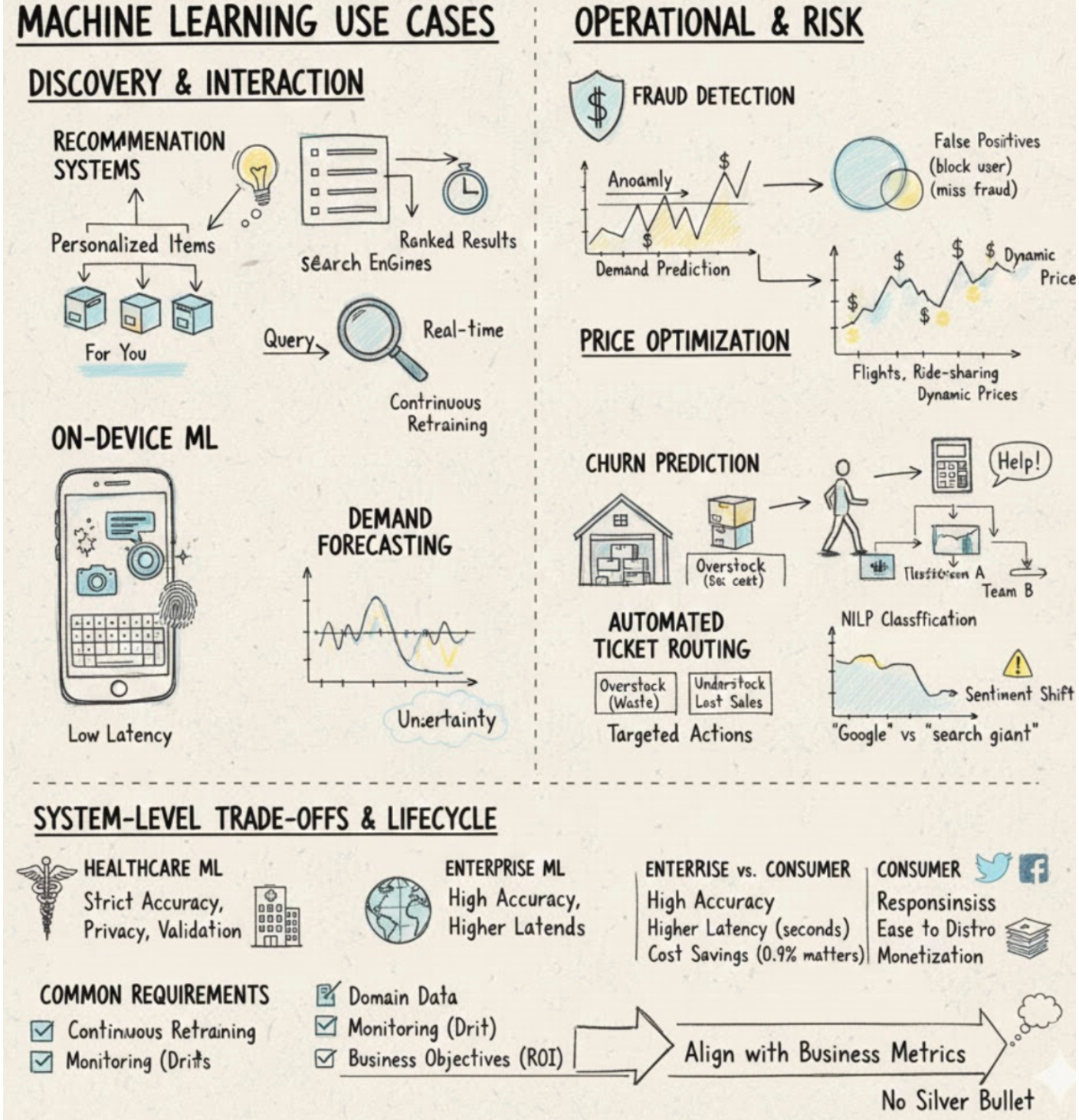
Organizations face two broad, recurring problems: how to help users find what they want amid overwhelming information, and how to make operational decisions that respond to changing demand and behavior. Machine learning addresses the discovery problem by powering recommendation systems and search engines that predict items or rank results to match user intent, reducing information overload and improving relevance. These are related but distinct applications: recommenders infer personalized items from behavioral signals, while search ranks content that matches a query. Both rely on large-scale user/item signals and real-time or near-real-time scoring pipelines to deliver timely, relevant experiences. In user-facing interfaces, on-device ML (examples: predictive typing, photo enhancement, fingerprint/face authentication) embeds models directly into UI/UX flows where low-latency inference and robustness to noisy input are required; this tight coupling with interaction design shapes constraints on model size, latency, and error tolerance.

Beyond discovery, ML tackles a range of operational and risk problems that require different modeling choices. Fraud detection typically blends anomaly detection with supervised classification over historical transactions; designers must trade off false positives (which block legitimate users) against false negatives (which miss fraud), and keep models resilient by continuously retraining on new fraud patterns. Price optimization uses demand predictions to set dynamic prices to maximize objectives like margin or revenue; it works best in high-volume, demand-fluctuating domains (ads, flights, accommodation, ride-sharing) and depends on throughput, accurate elasticity-of-demand modeling, and careful objective specification to avoid adverse business effects. Similarly, demand forecasting is a time-series problem used for stock and capacity planning: forecast errors lead to overstock (waste, perishables) or understock (lost sales), so models must quantify uncertainty and integrate tightly with inventory and budgeting systems. Customer lifecycle tasks are another common class: churn prediction estimates attrition likelihood to trigger targeted retention actions and can produce outsized financial gains because acquisition is expensive (for example, \$86.61 per paying app user or about \$158 per Lyft rider, and acquiring a new user costs 5–25× more than retaining one). Text-oriented problems such as automated ticket routing use classification and NLP to map support requests to teams, requiring labeled historical tickets, latency compatible with support workflows, and periodic updates for new issue types. For public-facing reputation monitoring, brand monitoring combines entity recognition and sentiment analysis to detect explicit and implicit mentions (for example, “Google” vs. “the search giant”) at scale over streaming social data and to alert on sudden sentiment shifts.

These use cases reveal recurring system-level trade-offs and lifecycle requirements. In regulated domains, healthcare ML demands stricter accuracy, privacy, and deployment constraints than many consumer apps; because failures carry safety and regulatory consequences, models are delivered via healthcare providers and require rigorous validation and privacy controls. More generally, enterprise customers often demand higher accuracy and can tolerate higher latency (where seconds may be acceptable), while consumer apps prioritize responsiveness and ease of distribution but face tougher monetization; as a result, even a small relative accuracy improvement (for example, 0.1%) can translate to large enterprise cost savings. Practically, most enterprise ML depends on domain-specific labeled or historical datasets (fraud logs, transaction volumes, support tickets, brand mentions), continuous retraining to adapt to distribution shifts, monitoring for drift and failures, and explicit integration with business objectives to measure ROI. Design decisions should therefore align latency, throughput, and model lifecycle practices with the specific business metric you intend to move—because the right technical trade-offs depend less on algorithmic novelty and more on fitting models into real operational and economic constraints.

Understanding Machine Learning Systems

Machine learning in production shifts the design conversation away from architectures alone and toward data as the primary design variable: the amount of data you collect, the quality and consistency of its labels, and the distribution it represents are often the levers that most strongly determine a model’s behavior. This matters because an ML system is not a single artifact but a pipeline where upstream choices feed downstream outcomes. To reason about that pipeline, it helps to decompose scope into data-centric stages (collection, labeling, validation), model-centric stages (training, evaluation), and system-centric stages (serving, monitoring, retraining). Each stage consumes the outputs of the previous one, so poor labeling or skewed collections propagate through training and surface as production failures. In contrast to academic ML, which optimizes for algorithmic novelty and benchmark scores, production ML must trade those research goals for operational constraints — latency, throughput, cost — and for robustness and maintainability. Likewise, unlike deterministic traditional software, ML components produce probabilistic outputs learned from data, which creates non-determinism, tight coupling to input distributions, and testing patterns that must be data-aware rather than purely unit-test driven.

Because model quality ties directly to the data pipeline and to serving infrastructure, responsibilities shift: data engineers and labelers, ML engineers, and SREs must collaborate closely. This leads to operational patterns and trade-offs you will make repeatedly. For example, you balance model accuracy against compute costs for both training and inference; you decide between replacing a model instantly (favoring consistency) or rolling it out gradually with canarying or A/B tests (favoring availability and risk control); and you weigh development speed against reproducibility and traceability, which drives data and model versioning. These lifecycle differences mean ML development is inherently iterative and continuous — collect data, retrain, redeploy — so you need automated retraining triggers, versioned datasets and models, and deployment practices that expect change. Without those practices, common ML failure modes emerge: dataset shift or concept drift where the input distribution moves over time; label noise that corrupts what the model learns; training-serving skew when features are computed differently in training versus production; and silent degradation, where performance erodes unnoticed. As a result, runtime monitoring, drift detection, and human-in-the-loop remediation become first-class operational requirements.

Performance and measurement considerations further separate ML systems from typical software projects. Training is largely compute- and IO-bound: throughput and distributed scaling determine how quickly you can iterate on large datasets. Serving, in contrast, is latency-sensitive — model size, batching behavior, and hardware choices directly affect P99 inference latency — so scaling strategies for training and serving diverge. Measurement also changes: research metrics and benchmark accuracy are necessary for model development but insufficient for production. You must instrument business-oriented metrics, run real-user experiments, and continuously monitor to detect regressions that static benchmarks miss. Taken together, these points motivate a systems-oriented treatment: production ML introduces system-level concerns — pipelines, monitoring, deployment patterns, and cross-functional roles — that mean traditional software engineering and ML research provide important tools but not a complete solution. Embracing that systems perspective lets you manage the trade-offs and operational risks that determine whether a model continues to deliver value after it leaves the lab.

Mind vs. Data

Machine learning teams routinely face a fundamental strategic choice: should they spend scarce engineering time encoding structure into models, or should they instead invest in collecting and computing on ever more data? Framing this as a choice between “mind” and “data” makes the trade-off explicit. “Mind” means deliberately building inductive structure into models — for example, using inductive biases, causal inference frameworks, or Bayesian networks — so systems can learn reliably from limited examples. “Data” means using simple, general-purpose learners and letting scale (more labeled examples plus more computation) discover patterns without heavy human encoding. This matters because, in realistic projects, neither time nor compute is infinite: where you allocate engineering effort determines whether your system will generalize efficiently from few examples or leverage massive data to outperform bespoke designs.

Understanding how these approaches work in practice requires looking at their resource and failure characteristics. A “mind”-first design increases sample efficiency: by constraining hypothesis space with structural priors or causal reasoning, you reduce the amount of data needed to generalize correctly. In contrast, a “data”-first strategy relies on sheer scale; as Richard Sutton argues, general methods that exploit compute and large datasets can win in the long run because they scale with available computation. But scale comes with costs: more data drives up storage, I/O, and compute demands and forces architecture choices such as distributed training and large-scale storage systems. Concrete benchmarks show how steep that scaling is: One Billion Words was roughly 0.8B tokens in 2013, GPT-2 about 10B tokens in 2019, and GPT-3 around 500B tokens in 2020. These numbers illustrate why a data-centric path requires substantial investments in pipelines and infrastructure.

From an engineering perspective, data work is foundational: advanced modeling is brittle without robust upstream systems. Monica Rogati’s Data Science Hierarchy of Needs — Collect → Move/Store → Explore/Transform → Aggregate/Label → Learn/Optimize → AI/Deep Learning — captures this dependency chain. Instrumentation, ETL, storage, cleaning, feature aggregation, and labeled datasets are prerequisites: if collection or labeling is poor, even the most capacious model produces garbage-in/garbage-out. Prioritizing data quality and quantity therefore implies heavy investments in logging, anomaly detection, labeling processes, and governance. Conversely, leaning toward structural modeling demands concentrated human effort to craft inductive biases and causal models, which reduces capacity to scale datasets and compute in the same time window. Christopher Manning warns of “bad learners” when algorithmic structure is too simple, while proponents of structural priors argue these designs outperform data-heavy approaches under finite-data regimes.

These trade-offs determine when each strategy is preferable and what risks you accept. When data is scarce or when safety and causal interpretability matter, favoring the “mind” — explicit structure and causal reasoning — improves sample efficiency and gives clearer failure modes. When large, high-quality datasets and ample compute are available and rapid empirical scaling is feasible, favoring the “data” approach can deliver superior performance but requires heavy investment in infrastructure and governance to avoid brittle systems. The debate also has temporal stakes: some predict structural methods will regain prominence quickly, others predict compute-leveraging general methods will eventually dominate, reflecting strategic uncertainty for where organizations should invest. In short, practical ML engineering is about balancing human design and data scale: choose structure to get more from less data, or choose scale and engineering to let general methods learn from abundance — but only after you’ve secured the foundational layers that make either path reliable.

Language model datasets over time (log scale)

Over the past decade the quantity of text used to train language models has not increased linearly but multiplicatively: on a log scale the exponential data growth is clear. This matters because larger training-data volumes are themselves a historical driver of progress in deep learning—many recent gains in model capability track closely with increased corpus size. In other words, feeding models much more data has been one of the principal levers for improving performance, and the dataset-size trend therefore shapes research choices and engineering priorities across model design, compute provisioning, and data collection.

At the same time, more data is not an unalloyed good. The relationship from raw data volume to accuracy is non-monotonic: simply adding examples does not guarantee better models. That arises from a classic quality-versus-quantity trade-off — when additional examples are lower quality they can actively harm learning rather than help. Two concrete failure modes illustrate why: outdated data, which creates a temporal mismatch between training and the current target distribution, and incorrect labels, which inject label noise into supervised signals. Outdated data produces a distribution mismatch that reduces generalization to present-day tasks, while incorrect labels produce noisy gradients that slow or misdirect optimization and corrupt the supervision the model needs to learn the right patterns.

These harms have practical consequences. Because training cost scales with dataset-size, ingesting large volumes of low-quality data increases compute, time, and monetary cost without commensurate gains and can reduce a model’s effective sample efficiency. As a result, exponential dataset growth forces stronger data engineering: freshness checks, label validation, filtering and deduplication become essential controls to prevent scale from producing regressions. Given limited compute and resources, the practical prioritization is clear—collecting and preserving high-quality, relevant data yields better returns than indiscriminate volume growth, and marginal low-quality examples can be net-negative to model performance.

Machine learning work in research and in production answers different questions, so they optimize for different outcomes. In research the priority is training throughput and experimental agility: you want fast training loops, many epochs, large batches, and tunable gradient-descent pipelines so you can compare algorithms on repeatable train/test splits. In production the priority flips to fast inference and low-latency, highly available responses for real users. As a result, architecture and resource allocation change: what looks like a distributed GPU/TPU cluster to maximize compute utilization in research becomes a highly responsive serving stack with horizontal replication, autoscaling, and tight latency SLOs in production. This mismatch also creates an evaluation gap—offline metrics that look good on a static test set often fail to predict real-world behavior when inputs are changing or models affect user behavior.

Thanks for reading! This post is public so feel free to share it.

To bridge that gap, production ML treats data and operations as first-class concerns. Because production data is non‑stationary, systems must continuously validate inputs, detect distributional changes, and keep features consistent across training and serving. This leads to a pipeline that connects ingestion → validation → feature materialization → training/serve, with components such as a feature store (for consistent feature materialization), data validators (schema and distribution checks), and drift detectors (statistical tests and thresholds). Production also integrates operational controls around fairness and interpretability—fairness audits, bias mitigation, and explainability tools become part of evaluation and monitoring, which adds latency and complexity but is operationally necessary. On the serving side, architects use model compression techniques (quantization, distillation, operator fusion, caching, sharding) to reduce inference cost and latency; these methods improve throughput but may degrade accuracy or interpretability, so they must be balanced against validation and rollback strategies. Similarly, batching incoming requests raises throughput at the cost of higher tail latency, forcing a trade-off between cost efficiency and SLA compliance.

Operational resilience and observability determine whether a deployed model stays useful. Production failure modes include dataset shift, train/serve skew (differences in feature computation between offline training and online serving), silent data corruption, feedback loops where the model changes the distribution it sees, and gradual model degradation. To mitigate those risks systems add end‑to‑end tests, feature validation, shadow or canary deployments, and automatic rollback procedures. Observability goes far beyond loss and accuracy: you must monitor latency and throughput, input feature distributions, label (ground‑truth) latency, model score distributions, fairness metrics, and relevant business KPIs, with tuned thresholds and alerting rules for drift sensitivity and degradation. Scaling strategies reflect different cost profiles: training is scaled out for throughput (data or model parallelism) and tends to be episodic and compute‑intensive, whereas serving is scaled out with replication and request routing and is a continuous cost-per-request. There is also a design choice between online learning (continual updates that reduce freshness lag but increase complexity and safety risks) and periodic retraining (simpler validation but slower adaptation). Finally, production ML embeds software-engineering practices missing from many research workflows — CI/CD for models, reproducible artifact storage and data lineage, controlled canary/A–B rollouts, and runbooks—to trade development velocity for governance and reliability. Taken together, these practices close the loop between offline research and live behavior, making ML systems maintainable, auditable, and robust in the face of real-world change.

Different stakeholders and requirements

Engineering teams rarely optimize for a single truth: product decisions sit at the intersection of many stakeholders with competing objectives. ML engineers want the best predictive accuracy, sales care about revenue per order, product owners impose strict latency targets, infrastructure teams demand reliability and maintainability, and management focuses on margins. These differing priorities create a situation where what looks like a better model on one axis can be objectively worse on another. For example, one approach (model A) might maximize click probability while another (model B) targets app revenue; because those objectives are orthogonal they produce different item rankings and even different model architectures. Without an explicit process to prioritize or reconcile objectives, teams will make deployment choices that satisfy some stakeholders while violating others.

A practical approach to this multi-objective tension is decoupling objectives: train specialized models for each stakeholder objective and combine their outputs downstream. That separation preserves interpretability — each model remains closely tied to a single business metric — and lets teams iterate independently. In practice, combining predictions then becomes a system-design problem: you must choose an aggregation strategy (for example, weighted scoring or constrained optimization), accept additional latency and complexity from multiple model calls, and maintain a clear contract about how trade-offs are resolved. This trade-off is particularly stark when product constraints are hard. If product requires a latency SLA of under 100 milliseconds and you know abandonment rises by 10% above that threshold, you must treat latency as a must-have constraint: higher-performing but slower models are effectively ineligible. If latency is only a nice-to-have, you can entertain slower models but only after quantifying the user impact.

Operational realities further constrain model design and rollout. Infrastructure teams who see nightly scaling alerts will prioritize platform stability and may freeze model updates to reduce operational risk; this creates a direct tension between model freshness/experimentation and reliability. Similarly, techniques that shine in research — ensembling being the canonical example — often increase prediction latency, system complexity, and maintenance cost. The Netflix Prize winners illustrate this: ensembling delivered better offline metrics but ensembles are rarely practical in production because of these operational costs. Deciding whether to accept that added complexity requires a cost–benefit judgment: a 0.2% lift in CTR might translate to millions of dollars and justify complex engineering, whereas a 0.2% absolute improvement in speech recognition from 95.0% to 95.2% is likely imperceptible to users and unlikely to justify extra latency, energy, or maintenance burden.

Finally, be wary of incentives and evaluation artifacts that mask true production value. Leaderboards and shared benchmarks invite multiple-hypothesis testing; when many teams evaluate on the same hold-out set, some reported gains are false positives and do not generalize to your production distribution. Benchmark-driven incentives (seen on platforms like GLUE and Kaggle and discussed in EMNLP 2020) push researchers to maximize single metrics—accuracy, for example—at the expense of deployability concerns such as compactness, fairness, or efficiency. The consequence is a catalog of production failure modes: increased latency, scalability breakdowns under traffic growth, harder debugging, higher energy consumption, and more frequent infrastructure interventions. To avoid these outcomes you must explicitly map stakeholder requirements to evaluation metrics, treat organizational incentives (including managerial cost-cutting or consolidation goals) as real constraints, and codify trade-offs so deployment decisions are defensible across teams.

Computational priorities

When you build machine learning systems, the dominant resource constraint shifts as the system moves from experimentation to production, and recognizing that shift is critical. In early development the bottleneck is development-phase bottleneck: you run many repeated training runs to tune hyperparameters and evaluate candidate architectures, so training wall-clock time and iteration throughput (how many complete training experiments you can run per day) directly govern developer productivity. To move faster you therefore optimize for metrics like time-per-epoch, convergence time, and the total number of experiments completed — improvements here shorten the feedback loop and increase experimentation velocity, which is the primary objective during model development.

This focus changes after deployment because serving predictions continuously becomes the dominant cost — the production-phase bottleneck. Production optimization targets are different: minimize inference latency, maximize throughput (requests/sec and concurrency), and reduce cost per million inferences while meeting SLAs. This lifecycle mismatch creates a real misprioritization risk: techniques that speed up development (for example, larger models that train better per experiment, expensive data augmentation that improves generalization, or heavy ensembling to boost validation scores) often increase inference compute, memory, and latency. As a result, a model tuned exclusively for fast training can become expensive or slow to serve, and conversely a model hand-optimized for minimal inference cost can slow down experimentation. To manage this trade-off, teams must treat serving efficiency — latency, memory footprint, and per-request compute — as first-class constraints during model selection rather than an afterthought.

Those different priorities imply concrete architecture, measurement, and CI choices. Resource provisioning should reflect phase: allocate cluster capacity and scheduling to support many concurrent or long-running training jobs in the experimentation environment, and provision latency-optimized, highly available serving infrastructure in the production environment to meet SLA requirements. Instrumentation must also follow the regime: development telemetry should emphasize time-per-epoch, convergence time, and experiments-per-day so you can detect slow feedback loops, while production telemetry should measure 95/99th percentile inference latency, throughput, request concurrency, and cost metrics to reveal serving bottlenecks. For reproducibility and CI, avoid re-running heavy training unnecessarily inside your continuous integration pipeline; instead scope automated tests to surface regressions cheaply, and design production CI/CD to validate inference performance (latency, memory, behavior under realistic load) not just accuracy on a test set. In practice this leads to an architectural pattern: treat the ML lifecycle as two distinct operating regimes — an experimentation environment optimized for fast training iterations and an isolated serving environment optimized for inference — so you don’t force a single design to serve two conflicting objectives.

Latency vs. throughput

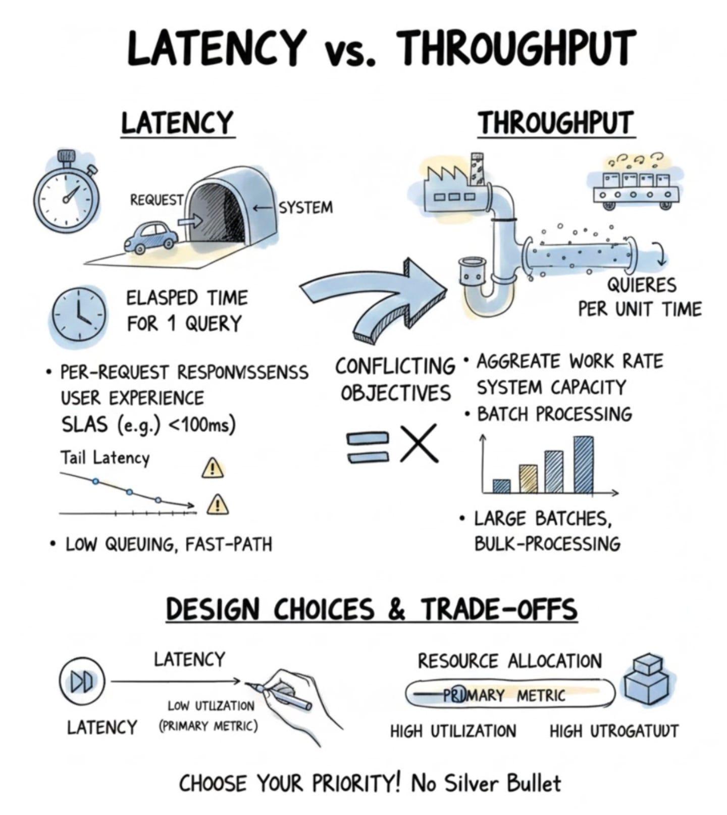
In distributed systems and services we care about two fundamentally different performance dimensions: Latency and Throughput. Latency measures the elapsed time for a single query — from when the system receives a request to when it returns a result — so it captures per-request responsiveness. Throughput measures the aggregate rate of work over time, i.e., how many queries the system processes per unit time, and therefore expresses capacity and volume. These two metrics answer different operational questions: latency tells you how quickly an individual user sees a response, while throughput tells you how much total work the system can absorb.

Because they answer different questions, systems optimize for one or the other in different contexts. Research systems and data-parallel experiments typically prioritize throughput: they want to process large volumes of data or drive high benchmark numbers, so designs emphasize batching and bulk-processing pipelines that maximize utilization. In contrast, production systems that serve real users prioritize latency and user-perceived responsiveness — often because of SLAs — so they favor low queuing, fast-path optimizations, and aggressive provisioning to keep per-request times down. This leads to divergent design choices: a throughput-oriented change (for example, introducing larger batches) increases aggregate work done per unit time but usually increases the per-request elapsed time; conversely, reducing queuing and over-provisioning lowers latency but reduces resource utilization and aggregate throughput.

Those divergent choices have clear resource-allocation and measurement consequences. Maximizing throughput typically raises utilization and amortizes fixed costs across many queries, which is economical for batch and benchmark workloads. Minimizing latency often requires accepting lower utilization: you may run more parallel, statically provisioned capacity or perform precomputation so individual requests see minimal delay. Correspondingly, the optimization targets differ: throughput tuning looks at aggregate rates and end-to-end capacity numbers, whereas latency tuning requires per-request timing, attention to tail-latency, and tight monitoring against SLAs. As a result, the instrumentation and feedback loops you build for each goal are different — one tracks average or sustained rates, the other tracks distributions and worst-case per-request times.

The practical takeaway is that you cannot generally maximize both simultaneously; they are often conflicting objectives. Therefore, when designing or tuning a system, explicitly choose which metric is primary and accept degradation in the other as a consequence. This means ranking objectives up front and letting that ranking drive architectural patterns (batch vs fast-path), resource allocation (high utilization vs reserved capacity), and which metrics you measure and optimize. Doing so makes trade-offs deliberate rather than accidental and aligns system behavior with the real priorities of research experiments or production user experience.

TERMINOLOGY CLASH

When engineers discuss performance they often run into a simple but consequential terminology clash: different authors define the same words differently. One common split contrasts Kleppmann’s usage, which separates response time (the client-observed, end-to-end interval that includes network, queueing, and service) from latency (just the service’s internal wait or processing time). This text instead collapses those terms and defines latency as the client-observed wall-clock interval from when a request is sent until a response is received — explicitly including network transfer, queueing, and processing — because that matches the machine-learning community’s usage and keeps discussions about user experience straightforward.

With that definition in place, the relationship between latency and throughput becomes easier to reason about. For a system that processes one request at a time, throughput is roughly the reciprocal of average latency: throughput ≈ 1 / average_latency, so 10ms average latency corresponds to about 100 queries/sec and 100ms to about 10 queries/sec. Introducing batching disrupts that simple inverse because the system processes multiple requests together. If a batch of 10 requests completes in 10ms, the average per-request latency remains 10ms while throughput jumps to about 1000 qps; if a batch of 100 takes 50ms, average latency becomes 50ms and throughput rises to 2000 qps. This gives a powerful lever to increase hardware utilization, but it comes with a key complication: online-batching requires the system to wait for enough arrivals to form batches, which adds queueing delay and raises client-observed latency. As a result, batching is a deliberate trade-off between raw throughput and the latency users experience.

Those trade-offs drive different priorities in research and production. Research work typically optimizes throughput — samples/sec — and will accept higher per-sample latency through aggressive batching to maximize hardware efficiency. Production systems, however, prioritize low user-observed latency because small increases in latency measurably hurt business metrics: studies show that 100ms extra delay can reduce conversions by about 7% (Akamai, 2017), modest latency increases can nudge conversion down (Booking.com, 2019), and page loads over 3s cause more than 50% mobile abandonment (Google, 2016). In practical terms, minimizing latency by processing single samples often underutilizes parallel hardware and raises cost per sample, while maximizing throughput with large batches improves utilization but can degrade user experience and therefore revenue.

Finally, it’s important to treat latency as a distribution, not a single scalar. Reporting only the arithmetic mean obscures tail behavior: a stream of requests that are mostly around 100ms plus one 3000ms outlier gives a misleading mean of 390ms even though most users see fast responses. For that reason, production teams prefer percentiles like p50/median, p90, p95, and p99 to describe what fraction of users see given latencies and to set SLOs (for example, p90 or p99.9 targets). Tail latency — the high-percentile behavior — matters because it affects a small fraction of users who are often disproportionately valuable, so engineering effort frequently targets those outliers. Operationally, percentiles help surface failure modes (sporadic network errors, transient delays) and guide remediation: if the mean rises because of systemic slowness you look for network or configuration fixes, whereas if the mean is high because of rare outliers you focus on identifying and eliminating those tail causes.

Data

Machine learning projects often start on tidy, well-understood benchmarks but run into trouble when they meet real users. Research datasets are static datasets: curated, cleaned, densely labeled, and packaged with preprocessing scripts that make model development fast and reproducible. Production data, by contrast, arrives as messy, unstructured, continuously generated inputs from users, systems, and third parties; it carries unknown biases, sparse or incorrect labels, and shifting distributions. This gap matters because models that perform well on clean benchmarks can fail unpredictably in the field, so teams must balance the short-term gains of reproducibility with the long-term need for representativeness.

Addressing that gap requires different data pipelines. Research workloads typically operate on historical or static repositories where quirks are known and preprocessing scripts suffice. Production systems must support both those historical stores and live streaming sources, which means building separate ingestion and processing paths for batch and real-time flows. Preprocessing in production must go beyond scripted transforms: it must clean malformed inputs, normalize unstructured formats, handle sparse/imbalanced/outdated labels, and support human-in-the-loop reannotation and label schema evolution. Because product-driven changes — for example adding or merging label classes — can happen after deployment, teams need coordinated schema/versioning strategies that cover label migration, dataset versioning, retraining, and downstream inference logic to preserve backward compatibility.

Operationalizing models against production data turns data issues into system failure modes. Unknown biases, noisy inputs, and sparse labels produce degraded or unpredictable model behavior unless you instrument for it: deploy continuous performance monitoring on live traffic, implement drift detection to identify distributional shifts, and define trigger conditions for retraining or human review so that newly labeled examples can flow back into training. These requirements interact with throughput and latency constraints: supporting high-throughput streaming and near-real-time model updates increases system complexity and cost, forcing trade-offs between processing expense and freshness of model updates. Data governance and privacy constraints further limit what can be collected, stored, annotated, or shared; they impose additional components such as access controls, anonymization, and legal review that shape the design of ingestion and debugging workflows.

In practice, follow an incremental strategy: use static benchmark datasets early for architecture search and controlled comparisons, then migrate to production-grade pipelines as you approach deployment so you expose the system to noise, bias, and streaming realities. Operational resilience comes from concrete investments: robust ingestion and validation to reject or flag malformed inputs, tooling for re-annotation and label merges, instrumentation to detect live degradation, and solid data/version management to enable rollbacks or retraining. As a result, teams move from evaluating models in the idealized loop dataset download → script-based preprocessing → offline training/evaluation to a production flow of streaming/historical ingestion → cleansing/normalization → sparse annotation/label management → monitoring and selective retraining → serving, with feedback loops for schema changes and privacy controls — a necessary evolution to make models reliable in the wild.

Fairness

Machine learning systems often inherit a structural bias: teams and research benchmarks reward improvements in narrow, measurable objectives such as accuracy or latency, so fairness becomes a secondary concern or an afterthought. This incentive structure — an incentive mismatch driven by a measurement gap — means researchers optimize what is measured, not what is equitable. As a result, models trained to minimize a global loss function will tend to underfit minority groups because errors affecting a small fraction of examples have little impact on aggregate metrics. This concentration of risk on underrepresented groups creates a predictable failure mode: a model can claim state-of-the-art performance while systematically disadvantaging people whose outcomes are invisible to the dominant optimization signal.

A core technical mechanism for that systematic harm is data bias and the related proxy-feature failure mode. Historical datasets encode social and systemic patterns — fields like zip_code, name spelling, or credit_score often act as proxies for protected attributes such as race or socio-economic status. Removing an explicit race field does not erase those correlations; unless you change the proxies or the data-generation process, models continue to reproduce and sometimes amplify discriminatory patterns. At scale this becomes scale amplification: what would have been isolated human errors now apply instantly to millions of cases, turning intermittent unfairness into pervasive, high-throughput discrimination.

Two practical consequences follow. First, aggregate metric blindness means that improving outcomes for a small subgroup can produce only a tiny change to global metrics, so organizations face a cost asymmetry: reducing misclassification for underrepresented groups typically requires expensive data collection, model adjustments, or constrained objectives while yielding marginal aggregate gains. This economic trade-off helps explain why many companies do not prioritize fairness — empirically reflected in cross-domain harms (loan and mortgage rejections, predictive policing, biased hiring tools, and skewed college rankings) and studies like the Berkeley estimate that roughly 1.3 million creditworthy Black and Latino applicants were denied mortgages between 2008–2015. Organizational readiness also lags: a McKinsey survey found only 13% of large firms actively addressing equity risks as of 2019.

Taken together, these points make a clear design imperative: fairness cannot be a retrofit. The aphorism “When it gets to production, it’s too late” captures why fairness must be embedded in data collection, objective specification, training pipelines, and evaluation from the start. Practically, that means adopting explicit fairness-aware objectives and benchmarks, evaluating targeted slices of the population rather than relying solely on global metrics, intervening in datasets to reduce proxy leakage, and documenting outcomes so external auditability and public evidence (as argued by critics like Cathy O’Neil and by academic case studies) can surface harms. These changes introduce trade-offs in cost and complexity, but they are the mechanisms available to convert fairness from an abstract ideal into measurable engineering practice.

Interpretability

Deciding whether to prioritize raw predictive performance or understandable explanations is a core engineering and policy problem for deployed ML. Geoffrey Hinton’s thought experiment — choosing between a higher-accuracy but opaque black-box system that achieves 90% cure versus a lower-accuracy but interpretable human at 80%—highlights this tension: optimizing for aggregate outcomes can conflict with the need for explanations that stakeholders trust, consent to, and can use to spot harms. Acceptance of opacity is not universal; a small survey of thirty technology executives split roughly half-and-half on whether they would accept the opaque, higher-performing system, showing that willingness to trade explainability for accuracy depends on human risk preferences and trust rather than raw metrics. This tension is also domain-dependent: like a microwave that users tolerate as an opaque appliance, life-critical settings such as surgery demand explainability for moral, legal, and psychological reasons.

Understanding what interpretability does helps resolve how to design systems around it. At a functional level, interpretability serves two complementary roles: for business leaders and end users it establishes trust and enables detection of biased decisions, while for developers it provides diagnostic signals to debug, find root causes, and iteratively improve models. In practice this means treat explanations not as cosmetic UI text but as an operational feedback channel: explanations feed audits and user trust upstream and provide actionable diagnostics downstream that close the loop between deployment and model updates. As a result, product and engineering teams must bake explainability into system requirements rather than leaving it optional — adding explicit interpretability objectives and evaluation criteria alongside traditional accuracy metrics prevents misalignment between research benchmarks and product needs.

Deploying that design choice has practical and governance consequences. Current incentives in ML research favor single-objective optimization for performance, so interpretability techniques remain underdeveloped relative to predictive gains; this incentive misalignment helps explain why only 19% of large companies were actively working to improve algorithmic explainability as of 2019, creating an adoption gap that raises operational and reputational risk. Choosing opaque, higher-performing models can increase aggregate utility but simultaneously reduce individual-level consent, obscure biases, and hide failure modes—preventing detection and remediation of harms even when aggregated metrics look strong. Because these trade-offs touch legal and policy questions (for example, whether opaque but effective systems should be permitted), engineers must treat interpretability as a cross-cutting requirement that influences architecture, evaluation, compliance, and stakeholder communication.

Discussion

Companies need machine learning to deliver near-term business impact, not just novel results on academic benchmarks. This creates a systemic gap between academic ML and industry needs: academic work often prioritizes novelty and long-term exploration, while businesses must justify investment with products, features, or measurable ROI. At the same time, modern research trends push toward “bigger, better” models that require massive quantities of data and, often, “tens of millions of dollars in compute.” That massive compute/data barrier raises a high fixed cost for anyone trying to produce state-of-the-art base models from scratch, making pure research an expensive proposition inside commercially constrained organizations.

As a result, the ecosystem splits into two complementary roles. Large, well-funded research labs concentrate on producing new base models because they can absorb the fixed costs, while downstream teams within companies focus on integrating and adapting those models for product use. This creates a practical pipeline: research produces pretrained/off-the-shelf models, organizations consume those models rather than re‑training, and production teams integrate them into systems. Because off-the-shelf models materially lower the entry cost, they shift investment away from reinventing cutting-edge training towards building the engineering that makes models useful in context.

That shift is a deliberate trade-off. Re-implementing cutting‑edge research internally can yield novelty but incurs high monetary and time costs; adopting pretrained/off-the-shelf models sacrifices some novelty in exchange for faster time-to-value and much lower training expense. For companies, the math favors adoption: short-term ROI pressures and budget constraints make production integration the more sustainable option. Consequently, the labor market follows—demand concentrates on productionizing ML: deployment, monitoring, reliable data pipelines, and adaptation of pretrained models into business workflows. These operational skills produce measurable outcomes and therefore align better with hiring needs than purely academic specialization.

This architecture has implicit consequences and failure modes. The “bigger” research strategy scales capability via compute and data but centralizes power among well-funded actors, reducing inclusivity for smaller teams and making in-house pure research financially risky. Attempting to run open-ended research inside a commercial team without a near-term product hook often becomes unsustainable and prone to cancellation. Therefore, a practical resilience strategy is to lean on the growing availability of off-the-shelf models and to prioritize engineering work that extracts business value through integration, reliability, and adaptation. For practitioners and organizations, that means allocating skills and effort toward deployment, observability, data infrastructure, and model adaptation — the areas that deliver industry relevance and keep ML investments aligned with business goals.

Machine learning systems introduce a fundamentally different engineering problem than traditional software because they are not just code — they are an interdependent bundle of code, data, and artifacts (the trained models) that together determine behavior. This tight coupling breaks the usual separation of concerns that software engineers rely on: you cannot reproduce or reason about a prediction by inspecting code alone if the training dataset and the specific model artifacts are not versioned and available. As a result, pipelines become workflows of code+data+artifact: trained models must be versioned, tested, and deployed alongside code, which complicates reproducibility, deployment, and maintenance in ways that go beyond traditional CI for source files.

Because business value often comes more from having the “most/best data” than from marginal algorithmic gains, system architecture shifts to treat data as a first-class component. Teams must prioritize data collection, storage, instrumentation, and fast integration into retraining pipelines so models can improve and adapt. That shift creates practical engineering questions: how do you version very large datasets, what test strategies validate data quality, and which samples deserve retention? Not all data points are equal — a rare cancerous scan is far more valuable than many normal scans — so blind accumulation can dilute signal or even enable attacks. This leads to explicit mechanisms for sample weighting, selection, curation, and strict ingestion policies. Without those controls, pipelines remain vulnerable to targeted backdoor or data-poisoning attacks (for example, poisoning a face recognition dataset to enable impersonation), so defenses such as data validation, anomaly detection, and controlled acceptance policies become part of the security surface.

The need for rapid adaptivity compounds these challenges. Data distributions change in production, so models require shorter retrain-and-rollout loops and CI/CD tailored to models; faster cycles keep accuracy but increase the risk of insufficient testing and instability. Operational constraints further shape design choices: modern models commonly span hundreds of millions to billions of parameters and require gigabytes of RAM to load, which constrains serving infrastructure and pushes trade-offs between accuracy and latency. Latency often acts as a hard correctness constraint for user experience — an autocompletion system that suggests answers slower than a user’s typing is effectively useless — so teams balance model size, resource allocation, and runtime optimizations to meet latency budgets. Pushing large models to edge devices is a massive engineering challenge: limited memory and compute, variable networks, and privacy considerations force choices among on-device inference, cloud serving, model compression, or split execution, each with distinct operational complexity.

These realities change what tooling and processes are necessary. Traditional software tools remain useful, but ML systems require additional capabilities: dataset versioning, data validation, model artifact registries, drift detection, richer telemetry (feature distributions, data-drift signals, model confidence), and model-serving orchestration. Observability and debugging become harder because learned behavior is less transparent than control flow; effective monitoring must expose data and model signals, not just logs and traces. The good news is that engineering investment can shift feasibility — models once thought too big for production (for example, BERT base at 340M parameters, ~1.35GB) are now deployed at scale through system-level optimizations — but that progress comes from integrating code, data, and artifact lifecycle concerns into architecture, tooling, and processes from the start.

Designing ML Systems in Production

Designing machine learning systems in production begins with a simple truth: this is a requirements-driven engineering activity. You are not picking models or servers in isolation — you are translating specified functional and non‑functional requirements into a concrete set of components and interactions that together implement an ML capability. To do that reliably you must treat the design surface as composed of five explicit component categories — interface, algorithms, data, infrastructure, and hardware — and map requirements (performance, latency, cost, safety, etc.) to concrete decisions for each category.

Each component has distinct responsibilities and downstream effects, so understanding those roles clarifies why design choices matter. The interface defines the boundary and contracts for inputs and outputs (for example APIs and data schemas) and is responsible for validating and transforming incoming signals and exposing model outputs in a usable form for downstream systems or users. The algorithms include the model and learning procedures; choices like architecture, training objective, and update cadence determine accuracy, latency, and resource demands, which in turn constrain infrastructure and hardware choices. Data is both training and serving data — its availability, quality, labeling strategy, and lifecycle (collection, validation, storage, versioning) directly influence model performance and repeatability. Infrastructure is the software stack for training/serving — orchestration, pipelines, storage, and monitoring — and its purpose is to connect interface, data, and algorithms reliably while providing operational properties such as throughput and scalability. Finally, hardware is the physical execution layer (CPUs/GPUs/TPUs/network/storage); selecting and configuring it is a cross‑cutting decision driven by algorithmic compute patterns and infrastructure throughput/latency targets. These components interact in a unidirectional logical flow — interface → data ingestion/validation → algorithms (training/serving) → outputs — with infrastructure and hardware supplying runtime, orchestration, and persistence; therefore you must specify both the components and the contracts between them explicitly.

Design is iterative because empirical behavior often violates initial assumptions. You validate an initial design against measurable requirements (for example throughput, latency, accuracy, data freshness) and then refine it: data drift, model generalization gaps, or unexpected cost/latency trade‑offs force changes to algorithms, data practices, or infrastructure. Improving one axis — say increasing model accuracy by using a larger model — has consequences on other axes (higher compute cost, increased latency, greater data needs), so designers must balance algorithmic choices, investments in data quality, and infrastructure/hardware budgets to meet the full set of requirements. A comprehensive design therefore produces concrete artifacts — interfaces/contracts, algorithm specs, data schemas and versioning policies, infra topology, and hardware profiles — and attaches measurable acceptance criteria to each artifact so teams can implement, test, and iterate objectively. Operational considerations such as deployment cadence, monitoring and retraining triggers, and failure/recovery behaviors are part of the design, not afterthoughts, because they determine whether the system can sustainably satisfy requirements once deployed.

Requirements for ML Systems

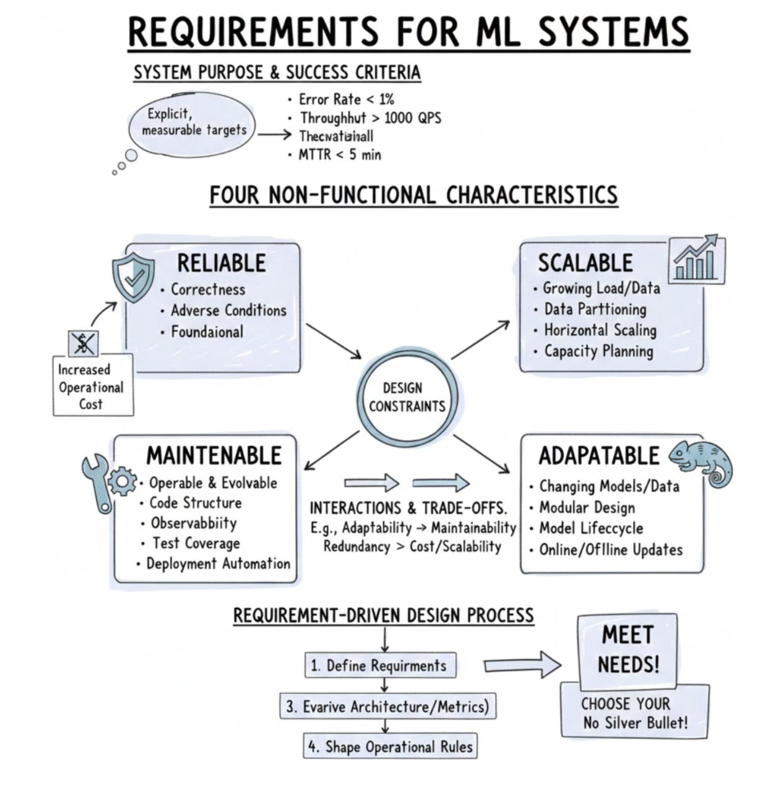
Before writing a single line of code, you must make the system purpose and success criteria explicit: clear requirements tell you what the architecture, implementation, and operations must deliver. Because different applications demand different behaviors, these requirements are use-case dependent — the acceptable trade-offs and numerical targets (for example, acceptable error rates, throughput, or MTTR) should be determined up front rather than assumed. Stating success criteria early forces your team to treat these targets as constraints that guide every subsequent decision, from component interfaces to runbook design.

To reason about those constraints, adopt a minimal baseline of four non‑functional characteristics you will evaluate your design against: reliable, scalable, maintainable, and adaptable. Reliability — the system’s ability to behave correctly under normal and adverse conditions — is foundational: if an ML service cannot be depended on, improvements in other areas are of limited value. Scalability captures the requirement to handle growing load or data volume and therefore drives concrete choices such as data partitioning, horizontal scaling strategies, and capacity planning. Maintainability focuses attention on making the system operable and evolvable over time; it manifests in code structure, observability, test coverage, and deployment automation. Adaptability prepares the system for changing models, data distributions, and requirements, which influences modular designs, explicit model lifecycle management, and whether you support online or offline update mechanisms. These axes interact: for example, designing for adaptability often improves maintainability, while adding redundancy to increase reliability can affect cost and scalability.

Making these requirements explicit up front also makes trade-offs visible. Prioritizing reliable behavior may increase operational cost or reduce development agility; conversely, optimizing purely for low cost can reduce resilience. Because of that, follow an ordered, requirement-driven design process: analyze each characteristic in turn (the document suggests walking through reliability first) and derive the concrete architectural patterns, metrics, and failure‑mode mitigations that meet your stated targets. The key takeaway is simple but powerful: define tailored, measurable requirements before construction, evaluate designs along the four baseline axes, and let those constraints shape architecture and operational rules so your ML system meets the real needs of its use case.

Reliability

Reliability means a system continues to perform the correct function at the desired level of performance despite adversity — and that adversity explicitly includes hardware faults, software faults, and human error. Framing reliability this way makes it a compound property: it’s not enough for a service to be “up” or to avoid crashes; it must both behave functionally correctly and meet performance or quality metrics that define acceptable behavior. For example, a call to model.predict() can complete without throwing an exception yet still produce outputs that fail to meet the system’s correctness or quality requirements, so runtime success by itself does not imply reliability.

This distinction becomes critical for machine learning systems because correctness is epistemically hard: in production there often are no ground-truth labels available to tell you whether a prediction is right or wrong. Traditional software failures tend to be explicit and observable — a crash, a runtime error, or an HTTP 404 provides an immediate signal you can detect and act on. In contrast, ML systems frequently suffer from silent failures: outputs degrade or become incorrect without any explicit error signal. As a result, naive monitoring that only checks availability or exception rates — standard health checks — can report a healthy service even when prediction quality has fallen below acceptable levels. This is compounded by the fact that API-level success (the API returning a response) is orthogonal to prediction accuracy, so common uptime-focused checks are insufficient for assessing ML reliability. Silent failures therefore carry high operational risk because end users may unknowingly accept and act on incorrect outputs — for example, receiving a flawed translation into a language they do not speak and thus cannot validate.

Because human error is a first-class failure mode alongside hardware and software faults, operational practices and humans-in-the-loop must be considered part of any reliability strategy. This leads to the need for production-focused analyses and strategies that go beyond conventional software reliability approaches: you must explicitly address how to detect and measure correctness when ground truth is absent, and how to mitigate the risk that incorrect outputs propagate unnoticed. In short, achieving reliability for ML systems requires treating correctness and quality as first-order outcomes, acknowledging the unique epistemic limits of predictions in production, and adapting monitoring and operational practices accordingly.

Scalability

Modern ML systems face a multi-dimensional scaling problem: they do not simply need “more servers” — they can grow along at least three orthogonal axes that demand different engineering responses. The first axis is model complexity: a system might evolve from a 1M-parameter logistic model to a 100M-parameter neural network, or from 1GB to 16GB of RAM per model. The second is traffic volume, where daily requests can move from 10k to 1M–10M. The third is model count, where a single model gives way to thousands of per-customer or per-feature models (for example, 8,000 models for 8,000 customers). Each axis changes the resource profile, orchestration demands, and operational practices in different ways — so understanding which axis is the primary pressure determines the correct investments.

At serving time you manage capacity with two basic resource actions: up‑scaling (allocating more compute/memory/GPUs) and down‑scaling (releasing resources when demand falls). The design goal is to match capacity to workload while meeting latency and throughput targets and minimizing cost. This trade-off is blunt: permanently provisioning peak capacity (for instance, keeping 100 GPUs always on) wastes money, whereas aggressive down‑scaling can leave you unable to absorb short spikes. Autoscaling exists to navigate that trade-off by sensing demand and adjusting capacity, but it introduces complexity and a critical failure surface. If the autoscaler is misconfigured, reacts to the wrong metrics, or scales up too slowly, the result can be downtime during peak events — as illustrated by Amazon’s Prime Day outage and its massive estimated cost — so autoscaling requires careful instrumentation, testing, and operational safeguards.

Model growth and traffic characteristics also change performance engineering choices. As model size increases, inference latency, memory footprint, and per-request throughput all shift, often pushing you to different instance types (GPU vs CPU), to batching strategies, or to model optimizations to meet SLAs. How you scale — the granularity of scaling — matters: scaling at the machine/VM/GPU level affects cold‑start time, billing granularity, and resource utilization. Fine-grained scaling reduces wasted capacity but increases orchestration overhead and potential instability. Likewise, autoscaling policies must be tuned for traffic-driven behavior: they should account for the rate of change, burst tolerance, scale-up speed, and cooldown windows; otherwise you either overspend or suffer dropped requests and high latency.

When the number of models grows, operational complexity multiplies. Moving from one model to N models makes ad‑hoc scripts and manual workflows untenable — you need automated lifecycle management for deployment, monitoring, retraining, and reproducibility. That requires deterministic artifact-management: track code, checkpoints, environment, and hyperparameters so models can be reproduced; experiment tracking and versioning become non‑optional when hundreds or thousands of artifacts exist. Monitoring and retraining must be automated too, with pipelines that detect drift, trigger retraining, and perform safe rollouts; without this automation mean time to recovery and operational cost rise sharply. Different scalability problems therefore map to different solutions: distributed training and model optimization address large-model and training-time pressure, autoscaling and resource management address serving-time capacity, and experiment tracking/versioning address artifact-scale. Finally, build resilience into each layer: conservative capacity buffers, canary rollouts, reliable artifact/version metadata, and end‑to‑end testing of autoscaling behavior mitigate key failure modes like autoscaler misbehavior, resource exhaustion during spikes, unreproducible artifacts, and monitoring blind spots.

Maintainability

Machine learning systems bring together people with different backgrounds — ML engineers, DevOps engineers, and subject-matter experts (SMEs) — who prefer different languages, tools, and workflows. This heterogeneity is a core maintainability problem because when each contributor tightly couples their preferred tools into a single pipeline, the result is brittle ownership, slow ramp-up for others, and painful incident response. To avoid that, you design the project and infrastructure so contributors can keep using familiar toolchains; letting people work in the environments where they are most productive reduces resistance to collaboration and raises velocity.

Achieving that flexibility in practice depends on providing tool-agnostic interfaces — stable, well-documented contracts that let different tools interoperate without tight coupling. Concretely, that means defining clear APIs, data formats, and integration points so components can be owned and developed in parallel. Paired with an explicit ownership model that assigns clear component and process responsibilities, these contracts prevent duplicated work, accelerate fixes by directing who should act during incidents, and make it easier to reason about cross-team dependencies. To diagnose problems across disparate components you also need consistent observability: standardized logs, metrics, traces, and error contexts that surface the same kinds of diagnostic signals regardless of the underlying toolchain. Standardizing telemetry has an implementation cost, but it pays off because teams can jointly investigate failures without guessing what to instrument next.

Allowing multiple toolsets buys autonomy at the cost of greater integration and testing complexity. Each additional tool requires connectors and increases the number of edge cases you must validate, so you balance freedom with a minimal set of mandatory shared contracts — enough to keep systems interoperable but not so many that you recreate a single monolithic toolchain. If an organization instead centralizes tooling or fails to provide shared interfaces, the architecture and culture encourage friction: slower incident response, blame cycles, and higher operational risk. To avoid that failure mode you need both the technical interoperability described above and social/process safeguards that steer collaboration away from fingerpointing toward joint diagnosis and remediation.

Finally, maintainability is as much about process as it is about APIs. As the number of contributors and toolsets grows, maintenance and integration testing costs rise nonlinearly, so pragmatic limits and minimal standards help contain operational overhead. Investing early in collaboration workflows, shared documentation, and post-incident collaboration norms reduces time-to-resolution and mitigates single-point-of-expertise (bus-factor) risks. In short, clear interfaces, defined ownership, standardized observability, and disciplined processes together turn a heterogeneous contributor base from a liability into a sustainable source of velocity.

Thanks for reading! This post is public so feel free to share it.

Adaptability

Machine-learned systems operate in a world where inputs and requirements shift quickly: changing customer behavior, upstream data schema changes, or new business goals can all erode model quality. If the system cannot detect those shifts and respond, model performance drifts silently and business metrics suffer. To avoid that, adaptability must combine two things: continuous discovery (detecting distribution drift, diagnosing bottlenecks, and surfacing problematic data slices or features) and the ability to apply fixes without interrupting service.

At the heart of this is the recognition that ML systems are part code, part data. Adapting a model therefore means more than swapping binaries — it requires managing changes to model code, the training_pipeline, and data artifacts such as feature encodings and data_contracts. This is why maintainability—modular code, clear data contracts, and reproducible pipelines—directly reduces time-to-adapt: cleaner modules let you iterate on a model component without touching serving infrastructure, and reproducible training artifacts let you validate fixes confidently before they leave the lab. Architecturally, this leads to a decoupled model lifecycle: separate training/validation from serving so teams can iterate on models and pipelines independently and shorten deployment cycles without increasing risk to live traffic.

Practically, non-disruptive updates rely on proven deployment patterns and strong instrumentation. Support for zero-downtime deployment means model versioning (model_version), and rollout strategies such as rolling updates, canary slices, or blue-green-like approaches, coupled with robust rollback_policys so regressions have low customer impact. Continuous monitoring and instrumentation surface what to update — whether a particular feature, a data slice, or a model component — and feed automated pipelines that can retrain and validate candidates. You must design for performance: minimize update latency (time from detection to deployed fix) while preserving serving throughput and latency, and scale ingestion and retraining capacity to match the rate of data change.

These choices have trade-offs. Pursuing rapid, zero-downtime updates increases operational complexity: orchestration, compatibility testing, and richer monitoring are necessary, and automation becomes essential to keep rollback and validation reliable. Configuration levers such as update cadence, detection thresholds for distribution shift, model validation acceptance criteria, and rollback policies determine where your system sits on the spectrum between agility and stability. In short, adaptability requires continuous discovery, a decoupled lifecycle that treats models and data as first-class artifacts, and investment in deployment patterns and tooling that make fast, safe updates possible.

Iterative Process

Machine learning development is inherently an iterative process rather than a linear project you finish once and forget. Because model behavior depends on choices across metric selection, data collection and labeling, feature engineering, training, evaluation/error analysis, and deployment, a change in any one area — for example a shift in labels, the data distribution, or business objectives — frequently forces you to revisit earlier steps. This matters because early design decisions, especially which metric you optimize, shape everything downstream: picking impressions as an objective will drive very different model behavior than optimizing CTR, and that choice can easily misalign with business outcomes such as revenue. As a result, teams should treat objective selection as a design decision with systemic consequences, and anticipate that business stakeholders may later demand a change in optimization target (for example moving from impressions to CTR), which cascades into data, features, model architecture, and evaluation criteria.

A disciplined loop relies on error analysis as the primary diagnostic layer: rather than blindly retraining, you investigate whether errors stem from label noise, class imbalance, feature gaps, or distribution shift, and then apply targeted fixes. Label quality is a first-class failure mode; discovered incorrect labels require relabeling and retraining because label noise biases learning and corrupts evaluation. Introducing human-in-the-loop relabeling reduces label noise but introduces cost and latency trade-offs. Severe class imbalance (for example, a dataset that is 99.99% no-show) systematically biases predictions toward the majority class; remedies include collecting more minority examples, resampling, reweighting the loss, or changing evaluation metrics — each option trades off data collection cost, training stability, and residual bias. Temporal issues are equally important: temporal distribution shift or concept drift (a model trained on “two months ago” data failing on “yesterday” data) means your evaluation sets must be recent and representative. Addressing drift requires fresher data, online or periodic retraining, or domain adaptation strategies, and each choice carries costs in compute, retraining frequency, and potential instability. In particular, test-set staleness produces overoptimistic metrics, so maintaining a rolling or held-out recent test set is required to measure real generalization to production.

Because deployment is not an endpoint, production introduces new observability and feedback requirements: you must continuously monitor both predictive performance and downstream business KPIs (for example impressions, CTR, revenue) so you can trigger retraining, adjust metrics, or make product decisions. The practical resilience strategies implied by this cycle include automated monitoring and alerts for performance degradation, pipelines for rapid data ingestion and labeling, retraining schedules or triggered retraining driven by drift detectors, and human-in-the-loop processes for label correction — all of which add operational cost but increase robustness. Importantly, error diagnoses map to concrete remediation actions: wrong labels → relabel and retrain; class skew → collect more positives or rebalance; recent degradation → collect fresh data and retrain; business metric change → redefine the loss/metric and retrain. Architecturally, supporting this loop requires orchestration layers — a data pipeline, labeling service, training pipeline, and deployment/monitoring stack — that enable frequent iteration. Design trade-offs here include how much to automate (fully automated retraining versus manual gating), update latency, reproducibility, and rollback capability. The key takeaway is that reliable ML systems treat iteration and diagnostic-driven fixes as core features: they are designed to detect problems quickly, map errors to targeted remedies, and accept the operational costs necessary to keep models aligned with changing data and business goals.

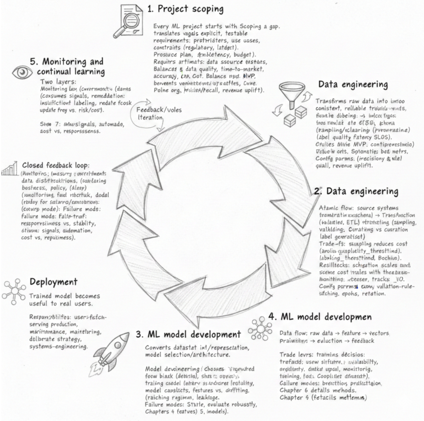
Step 1. Project scoping

Every ML project starts with a gap between a high-level business desire and the concrete engineering work needed to deliver it. Project scoping closes that gap by translating vague goals into explicit, testable requirements: measurable success criteria, prioritized use cases, and a clear list of constraints (regulatory, latency, budget, privacy). As a result, teams can size and prioritize downstream activities — data collection, model design, and engineering — because scoping produces the artifacts decision-makers actually act on: a resource plan (personnel, compute, storage, labeling), a stakeholder map assigning responsibilities and authority, and the KPIs/SLOs that define go/no-go decisions.

Turning a scope into an implementable plan requires concrete estimates and architectural choices. Scoping identifies expected data sources, ETL complexity, and labeling workflows, and measures data volume and freshness, storage needs, and compute costs (including FLOPs for training and inference). Those estimates directly shape model selection (a simple model vs. heavy deep learning), infrastructure patterns (batch ETL vs. streaming), and deployment location (on-prem vs. cloud), because decisions like using an online feature store or building real-time inference depend on captured constraints such as latency SLOs, data availability, and retention policies. In practice this also surfaces operational requirements—throughput targets, model update cadence, acceptable downtime—and the monitoring, provenance tracking, and capacity planning needed to meet them.

Scoping makes trade-offs explicit so teams can manage risk instead of reacting to surprises. Balancing business value and time-to-market against accuracy and cost leads naturally to an iterative path: define an MVP with minimal technical scope, include contingency buffers in budget and schedule, and set clear KPI-linked go/no-go criteria and timeline checkpoints. Poor scoping commonly produces underestimated data quality problems, missed legal constraints, insufficient labeling budgets, ambiguous ownership, or unclear KPIs — outcomes that delay delivery or produce models that don’t meet business needs. To prevent that, scoping should prescribe team organization (centralized ML teams versus embedded cross-functional squads), enumerate roles (data engineers, ML engineers, annotators, product owners), and set measurable configuration parameters — target precision/recall, revenue uplift, compute budget, dataset coverage, and labeling throughput—so procurement, staffing, and architecture follow from requirements rather than guesswork. In short, rigorous scoping converts business intent into verifiable engineering commitments and creates the guardrails needed to prioritize effort and surface risk early.

Data engineering

Machine learning development starts with a practical problem: raw, heterogeneous data from many systems is useless to a model until it is transformed into a consistent, reliable training dataset. This is the role of Data engineering — it solves ingestion, normalization, sampling, and labeling so models can learn from examples that are both meaningful and reproducible. In practice you move data along an atomic flow: source systems feed into ingestion connectors, those streams undergo format normalization and schema alignment, then validation and cleaning remove obvious errors, sampling and subsampling reduce volume, and finally label generation (manual or programmatic) produces the curated training set that goes into model training.

To make that flow manageable and auditable, teams adopt a pipeline-oriented ETL/ELT architecture that explicitly separates concerns. The first layer — extraction — relies on modular ingestion connectors that handle different source protocols and formats so you can plug in databases, logs, or object stores without changing downstream logic. The second layer performs transformation: schema mapping, type conversions, and validation rules detect and correct incompatible formats or missing metadata. The third layer focuses on curation and labeling: sampling policies, filtering rules, and label-generation logic (human tasks or heuristics) decide which examples are promoted into training datasets. This layered separation produces repeatability and provenance: when something goes wrong you can trace whether the issue originated in the connector, the normalization step, or the labeling step.

Design choices in each layer create explicit trade-offs you must manage. Sampling reduces storage, compute, and labeling cost, but it also introduces selection bias and increases variance; treating sampling_rate as a primary configuration knob makes that trade-off direct and observable. Labeling is another key trade-off: manual labeling yields higher quality at higher cost and latency, while programmatic or heuristic labeling lowers cost but raises label noise; this choice drives what validation and quality-control mechanisms you need and where to set label_quality_threshold for promoting examples to training. Performance bottlenecks commonly appear at ingestion throughput and storage I/O, while labeling speed (human throughput or compute for programmatic labelers) and transformation compute determine end-to-end dataset freshness and pipeline latency. To scale, you parallelize connectors, use distributed storage, choose batch versus streaming pipelines depending on freshness needs, and horizontally scale transformation and validation tasks to handle varied formats and higher volume.

Real systems also need resilience against typical failure modes: corrupted or incompatible formats, missing schema metadata, label noise, and sampling bias. Mitigations are practical: strict schema validation and typed conversions catch incompatible inputs early; provenance tracking records where each example came from and which transformations it underwent; label quality monitoring detects drift and data-quality regressions so you can retrain or relabel proactively. Configuration parameters — sampling rate, validation-rule strictness, label quality thresholds, and retention/partitioning policies — tie directly to cost, robustness, and recomputation overhead, so choose them with the pipeline’s operational goals in mind. The result is a data-engineering pipeline that explicitly balances representativeness, cost, and freshness while providing the repeatability and auditability required for reliable model training.

ML model development

At this stage you convert the raw training dataset into actual predictive capability: you extract informative inputs from the data and build first-pass models that can be evaluated and iterated. The minimal pipeline you implement here consists of feature extraction/representation, model selection and architecture, the training procedure, and evaluation. These stages form a tight data flow — raw data becomes feature vectors, those vectors feed training, the resulting predictors are assessed by evaluation, and the evaluation signals guide further work — so designing clear interfaces between stages makes iteration practical.

Two activities dominate the work and the decisions you make. First, feature engineering turns raw signals into the structured inputs that determine the signal available to models: feature quality directly constrains achievable performance and even the kinds of models that will succeed. Second, model development chooses model families and initial architectures and capacities that can leverage those engineered features; this produces the first working predictors you will analyze. Together these components expose the main configuration levers you will tune: which variables and transformations to include (feature choices and dimensionality), model hyperparameters like capacity and regularization, and the training regimen (batching, epochs). Because these choices interact — richer features can shift what model families perform well, and different regularization or capacity settings alter generalization — this stage demands substantial ML judgment rather than mechanical tool-running.

These decisions involve clear trade-offs and predictable bottlenecks. You must balance feature complexity against data sparsity because richer, high-dimensional features can overfit when data are limited; likewise, increasing model capacity can improve fit but also fits noise and harms generalization. Computationally, model training cost and convergence time scale with dataset size and feature dimensionality, and feature extraction itself can dominate preprocessing latency and memory/IO during training. Anticipate failure modes such as systematically biased predictions from poor features, underfitting or overfitting relative to available data, and leakage between training and evaluation stages that produces misleading metrics. Practically, be resilient by building simple baseline models first, evaluating them robustly, and using evaluation feedback to prioritize targeted feature changes or a shift in model class rather than rewriting everything. Finally, treat this stage as a signpost: it points toward deeper work — chapter 4 will dive into feature engineering detail and chapter 5 will cover model selection, training, and evaluation — reflecting a separation of concerns and a staged deepening of the development effort.

Deployment

Deployment answers a straightforward but critical question: how does the trained model become useful to real users? At this stage the primary technical goal shifts from improving model quality to providing operational access — making predictions, serving results, and exposing interfaces that users or downstream systems can call. Treating deployment as a release milestone helps clarify intent: launching the system is a deliberate decision point that separates the development phase from ongoing production operation, not a signal that the work is finished.

Because machine-learned systems are inherently iterative, deciding when to deploy involves a clear trade-off. You can ship a working but imperfect system to gather real-world feedback more quickly, or delay release to pursue further improvements offline. This leads to different risk profiles: early release accelerates learning through production telemetry and user feedback, while later release can reduce obvious failure modes at the cost of slower insight into real usage. As a result, deployment planning must include mechanisms for continuous updates, feedback loops, and change management so that the model can evolve after it goes live.

Choosing how to deploy is a systems-engineering decision that extends well beyond model training. There are different deployment patterns and strategies, each with distinct properties and trade-offs, and selecting among them requires deliberate evaluation against operational goals. Making a model accessible creates concrete responsibilities: user-facing interfaces must be designed, availability and uptime must be assured, and ongoing maintenance processes must be established. In other words, deployment is about integrating the model into production infrastructure and workflows — things like monitoring, rollback procedures, and update mechanisms become part of the engineering surface area even if the specific methods are addressed elsewhere.

Deployment has enough complexity that detailed technical approaches deserve a focused treatment; those methods are deferred to Chapter 6, which will dig into dimensions such as performance, reliability, integration, and update mechanisms. For now, the key takeaways are clear: view deployment as a milestone that enables real use and real feedback, plan explicitly for the continuous lifecycle that follows, choose your deployment strategy deliberately based on operational trade-offs, and accept the systems-engineering responsibilities that come with putting a model into production.

Monitoring and continual learning

Machine-learned systems in production face a persistent problem: performance decay. Models that once met accuracy, latency, or fairness targets often degrade over time because the world they operate in changes. These degradations come from two distinct root causes that require different responses: changing environments — for example, shifts in input or data distributions — and changing requirements — such as new business metrics or policy/regulatory shifts that redefine what “good” behavior means. Recognizing which cause is responsible matters because correcting for a transient distributional shift differs from re-aligning a model to new business priorities.

To address this, you need two tightly integrated but conceptually separate layers. The first is a monitoring or observation layer that continuously measures runtime performance and produces actionable signals — not just raw metrics, but alerts and contextualized indicators that a specific problem exists. The second is a maintenance or continual learning layer that consumes those signals and decides on remediation: retrain on fresh data, fine-tune model weights, roll back to a previous version, or change model behavior or thresholds. This separation between detection and remediation logic helps keep monitoring focused on reliable, explainable signals while allowing remediation policies to encode cost, risk tolerance, and business priorities.

Architecturally, the pattern that emerges is a closed feedback loop: production -> monitor -> update -> deploy. This loop enforces continuous validation and remediation instead of treating deployment as a one-time event. As a result, systems can adapt to both environmental drift and evolving requirements through iterative updates. However, this adaptivity introduces a trade-off between responsiveness and stability: updating frequently reduces the window during which performance drifts, but it increases the risk of overfitting to transient noise and raises operational costs; intervening seldom preserves stability and reduces false alarms but lets degradation persist longer. A common and dangerous failure mode is undetected drift — without effective monitoring, latent decay can propagate incorrect outputs into downstream decision-making. Therefore, monitoring must surface actionable, contextualized signals, and the maintenance pipeline must apply clear decision logic about when and how to act.

Continual learning in production is not a one-off patch; it is an ongoing element of model lifecycle management that iterates as environments and requirements change. This step therefore sits within the broader lifecycle: expect to formalize policies, thresholds, and automation patterns that govern detection and remediation. Those operational and technical specifics — how to set thresholds, when to automate retraining, and how to balance cost versus responsiveness — are treated in detail in chapter 7. In the meantime, the essential takeaway is that effective production safety and performance rely on a monitored, closed-loop process that turns observations into disciplined, repeatable maintenance actions.

Business analysis

Models can be technically excellent but still fail to move the business needle; Business analysis exists to bridge that gap by evaluating model performance against explicit business goals. This step translates raw, model‑centric metrics — things like accuracy, latency, or AUC — into meaningful business KPIs such as revenue lift, cost reduction, or churn reduction so stakeholders can interpret model behavior in value terms. By framing evaluation around the outcomes the company cares about, teams generate actionable insights that inform strategic decisions rather than producing isolated technical scores.

To make those insights operational, the analysis converts evaluation results into clear decision endpoints that act as go/no‑go signals: continue, scope further work, or kill the project. Those endpoints arise from quantified expectations of impact and feasibility, so prioritization and scoping follow directly from estimated value, required resources, and technical readiness derived from the model evaluation. This requires formal governance thresholds — numeric accept/continue/kill rules — that remove subjectivity and ensure portfolio actions are repeatable. Because business priorities and success criteria evolve, Business analysis establishes a bi‑directional feedback loop with Step 1: findings from model evaluations refine problem definitions and success metrics, and revised goals change how models are built and assessed. As a result, this step is not a one‑time audit but part of an iterative lifecycle (see chapter 9) that recurs as models and business objectives change.

Implementing this step has practical and managerial implications. Teams must capture both model performance data and corresponding business outcome data, and maintain tooling and processes that reliably compare those streams over time — enabling reproducible decisions and trend tracking. The analysis also forces explicit trade‑offs: should you invest to eke out marginal model improvements, or redeploy resources to higher‑value initiatives? Making those opportunity costs visible prevents continuing low‑value models by default. Without this alignment, projects risk remaining technically sound but business‑irrelevant; with robust measurement, governance, and a feedback loop, Business analysis turns model results into portfolio decisions that drive measurable business impact.

Summary

Deploying machine learning in the real world is not just about choosing the best algorithm; it is about engineering a multi-component system that reliably transforms raw data into business value. In practice, success requires coordinating distinct responsibilities: data engineering (ingestion, cleaning, and feature pipelines) prepares and shapes inputs; online vs. batch prediction defines serving modes — online prediction answers individual, low-latency requests while batch prediction processes large volumes periodically; deployment handles integration and rollout into existing services; monitoring watches model performance and detects data or concept drift; and maintenance manages model updates and lifecycle tasks. Each component matters because it addresses a specific failure mode or operational need that pure algorithmic work does not cover.

Those operational needs change the trade-offs engineers make. Production environments involve different stakeholders, different computational priorities, different data properties, more acute fairness concerns, and stricter interpretability requirements than academic research — five axes that push architectures and processes in different directions. Moreover, most production ML is enterprise rather than consumer-facing, which increases stakeholder diversity and operational constraints and often demands hybrid solutions where ML complements business logic rather than replacing it. Because ML is not a universal solution, systems should be designed to allow partial or mixed approaches where models provide probabilistic inputs to broader decision workflows.

A central practical debate — the data-versus-algorithm trade-off — has shifted toward data in recent years: high-profile wins such as AlexNet, BERT, and GPT illustrate how scaling data and training infrastructure can drive large gains. As a result, much of the engineering effort in production systems focuses on concrete data questions: how to acquire, validate, version, and pipeline large datasets so models can realize their potential. This perspective motivates an architectural style based on modular composition: building complex ML systems from simpler, well-scoped blocks so teams can separate concerns, iterate incrementally, and apply targeted operational practices to each block. Following this overview, the material proceeds into those building blocks beginning with data engineering, signaling that robust data infrastructure is the foundational layer for reliable production ML.

Download Source code usig the button below:

$ \mathbb{U} \int \varepsilon \quad \left[ \frac{ \tau \hbar e }{ \beta \cup \tau \tau \odot \eta } \right]_{\mathbf{b} \epsilon \ell \odot \omega} $

Beyond the Model: The Hard Truths of Deploying ML in Production

Why Algorithms Are Not Enough: A Guide to the ML Pipeline

This is only the first chapter. To access the complete book, download the full PDF using the button provided at the end of this article.

When to Use Machine Learning

Complex: the patterns are complex

When to Use Machine Learning

Complex: the patterns are complex

Patterns: there are patterns to learn

Predictions: it’s a predictive problem

Unseen data: Unseen data shares patterns with the training data

It’s repetitive

The cost of wrong predictions is cheap

It’s at scale

The patterns are constantly changing

Machine Learning Use Cases

Understanding Machine Learning Systems

Mind vs. Data

Language model datasets over time (log scale)

Different stakeholders and requirements

Computational priorities

Latency vs. throughput

TERMINOLOGY CLASH

Data

Fairness

Interpretability

Discussion

Designing ML Systems in Production

Requirements for ML Systems

Reliability

Scalability

Maintainability

Adaptability

Iterative Process

Step 1. Project scoping

Data engineering

ML model development

Deployment

Monitoring and continual learning

Business analysis

Summary

Download Source code usig the button below:

This post is for paid subscribers