


Build Your Own Image Classifier- Train a CNN on CIFAR-10
Build Your Own Image Classifier- Train a CNN on CIFAR-10
A Comprehensive Guide to Building and Optimizing CNNs with CIFAR-10 Dataset

Dive into the world of Convolutional Neural Networks (CNNs) with our detailed guide on building and optimizing your own image classifier using the CIFAR-10 dataset. This journey will take you through the nuances of setting up your coding environment in Google Colab, understanding the intricacies of implementing convolutional and pooling layers, and the significance of batch normalization in enhancing network performance. Whether you’re a beginner or an experienced practitioner, this guide offers a step-by-step approach to mastering CNNs, from basic layer implementation to fine-tuning and debugging for optimal results. Get ready to harness the power of CNNs and unlock the potential of image classification with hands-on examples and practical insights.
# this mounts your Google Drive to the Colab VM.
from google.colab import drive
drive.mount('/content/drive', force_remount=True)

# enter the foldername in your Drive where you have saved the unzipped
# assignment folder, e.g. 'cs231n/assignments/assignment3/'
FOLDERNAME = 'cs231n/assignments/assignment2/'
assert FOLDERNAME is not None, "[!] Enter the foldername."

# now that we've mounted your Drive, this ensures that
# the Python interpreter of the Colab VM can load
# python files from within it.
import sys
sys.path.append('/content/drive/My Drive/{}'.format(FOLDERNAME))

# this downloads the CIFAR-10 dataset to your Drive
# if it doesn't already exist.
%cd drive/My\ Drive/$FOLDERNAME/cs231n/datasets/
!bash get_datasets.sh
%cd /content
It imports the Google Drive module from the google.colab library. In the second line, the Google Drive is mounted to the Colab virtual machine VM and forced to be remounted if it is already mounted. Colab can access files and folders from the user’s Google Drive using this code. As part of the code, the user must enter the folder name in their Google Drive where they have saved the unzipped assignment folder. If the foldername is empty, it raises an error. For the next step, the correct folder is accessed. Afterward, the code imports the sys module and adds the user’s Google Drive path to the system path. Colab VM’s Python interpreter is able to access and load Python files within the specified folder. Following that, the code downloads the CIFAR-10 dataset to the user’s Google Drive if it doesn’t already exist. It is commonly used in computer vision tasks, and the code downloads it to the specified location. Lastly, the code sets the current working directory to the specified folder in the Google Drive so it can access files in that folder and work with them within Colab.
Download the source code from the link in comment section. If the link is not there that means I working I will post it till 5 Jan 2024.
Implementing Convolutional Networks
We’ve previously delved into deep fully-connected networks, utilizing them to delve into various optimization techniques and architectural designs. While fully-connected networks provide an efficient platform for experimental purposes due to their computational simplicity, the cutting-edge achievements in the field are predominantly achieved through convolutional networks.
Your initial task will be to develop a series of layer types commonly employed in convolutional networks. Subsequently, you will apply these custom layers to construct and train a convolutional network, specifically targeting the CIFAR-10 dataset for practical application and testing.
# As usual, a bit of setup
import numpy as np
import matplotlib.pyplot as plt
from cs231n.classifiers.cnn import *
from cs231n.data_utils import get_CIFAR10_data
from cs231n.gradient_check import eval_numerical_gradient_array, eval_numerical_gradient
from cs231n.layers import *
from cs231n.fast_layers import *
from cs231n.solver import Solver

%matplotlib inline
plt.rcParams['figure.figsize'] = (10.0, 8.0) # set default size of plots
plt.rcParams['image.interpolation'] = 'nearest'
plt.rcParams['image.cmap'] = 'gray'

# for auto-reloading external modules
# see http://stackoverflow.com/questions/1907993/autoreload-of-modules-in-ipython
%load_ext autoreload
%autoreload 2

def rel_error(x, y):
  """ returns relative error """
  return np.max(np.abs(x - y) / (np.maximum(1e-8, np.abs(x) + np.abs(y))))
To begin, we import the necessary libraries such as numpy and matplotlib, as well as various custom functions from the cs231n package. In addition, it allows external modules to be loaded automatically and sets some default plot configurations. After defining rel_error, we define a function. Using this function, you take two arrays, calculate their absolute difference, and then divide it by their maximum absolute value. The reason for this is to handle the case where one of the arrays or both arrays contain values that may result in a division by zero.
This value is the relative error between the two arrays, which can be useful for comparing calculation accuracy. It’s likely that the main purpose of this code is to set up and configure a convolutional neural network CNN for use with the CIFAR-10 dataset. In this dataset, there are 10 categories of images. As an example, the code may be used to train and test a CNN on subsets of the CIFAR-10 dataset for image classification. The Solver class is responsible for optimizing the CNN training process, while the eval_numerical_gradient and eval_numerical_gradient_array functions are used to evaluate gradient calculations. For tasks such as image classification, this code serves as a foundation for building and training a CNN on the CIFAR-10 dataset. It imports the necessary libraries, sets some default configurations, defines helpful functions, and imports custom code.
# Load the (preprocessed) CIFAR10 data.

data = get_CIFAR10_data()
for k, v in data.items():
  print('%s: ' % k, v.shape)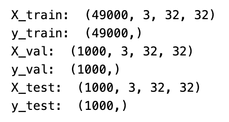
Data is loaded from the CIFAR10 data variable, which has already been preprocessed. There are various keys and values in the data variable, where each key represents a different aspect of the data, such as training images, training labels, test images, test labels, etc. Each key-value pair in the data dictionary is iterated through using the for loop, and the key and the shape of the corresponding value are printed on each iteration. Since the values are arrays, the shape refers to their size and dimensions. It simply displays information about the data loaded, such as the number of images and labels in the training and test sets.
Implementing Convolution: Basic Forward Pass
At the heart of a convolutional network lies the pivotal convolution operation. Within the cs231n/layers.py file, your task is to code the forward pass for the convolution layer in the conv_forward_naive function.
Focus on clarity and understanding in your implementation, rather than efficiency. This is an initial step, so it’s more important that your code is comprehensible and accurate.
To verify the functionality of your implementation, you can execute a test run as follows:
x_shape = (2, 3, 4, 4)
w_shape = (3, 3, 4, 4)
x = np.linspace(-0.1, 0.5, num=np.prod(x_shape)).reshape(x_shape)
w = np.linspace(-0.2, 0.3, num=np.prod(w_shape)).reshape(w_shape)
b = np.linspace(-0.1, 0.2, num=3)

conv_param = {'stride': 2, 'pad': 1}
out, _ = conv_forward_naive(x, w, b, conv_param)
correct_out = np.array([[[[-0.08759809, -0.10987781],
                           [-0.18387192, -0.2109216 ]],
                          [[ 0.21027089,  0.21661097],
                           [ 0.22847626,  0.23004637]],
                          [[ 0.50813986,  0.54309974],
                           [ 0.64082444,  0.67101435]]],
                         [[[-0.98053589, -1.03143541],
                           [-1.19128892, -1.24695841]],
                          [[ 0.69108355,  0.66880383],
                           [ 0.59480972,  0.56776003]],
                          [[ 2.36270298,  2.36904306],
                           [ 2.38090835,  2.38247847]]]])

# Compare your output to ours; difference should be around e-8
print('Testing conv_forward_naive')
print('difference: ', rel_error(out, correct_out))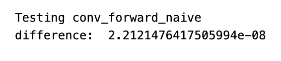
A convolutional neural network is created by creating the necessary variables, inputs, and parameters. X_shape describes the shape of the input data 2 examples, 3 channels, 4 rows, 4 columns; w_shape describes the shape of the filter weights 3 filters, 3 channels, 4 rows, 4 columns. With numpy’s linspace function, numbers are generated evenly spaced and assigned to x and w variables. Each filter has a b variable that represents the bias terms. In the conv_param variable, the stride and padding parameters are stored as a dictionary. A step is defined as how many pixels the filter moves at a time, and a padding is defined as how many rows and columns of zeros are added to the input data to allow more movement beyond the boundaries.
This code does not show the conv_forward_naive function, which convolutions the input data with weights, bias terms, and parameters. In the following code, the out variable holds the output of the function, and the underscore indicates the second output will not be used. This variable is used to test whether the function is correct by comparing the expected output to the actual output. Using rel_error, you can calculate how close the outputs are by calculating their relative error between two arrays. A convolutional neural network is setup and tested using Numpy in this code. Using these variables and inputs, it uses the convolution operation and compares the output to a manually calculated value to ensure that the function is correct.
Exploratory Activity: Image Processing Using Convolutions
In a blend of verification and learning, we’ll embark on an engaging task to explore the capabilities of convolutional layers. This involves preparing an input consisting of two images, and then manually configuring filters to execute standard image processing tasks, such as converting to grayscale and detecting edges. These filters will be applied to each image through the forward pass of the convolution. The outcome can then be visualized, serving as a practical and insightful sanity check.
Colab Users Only
# Colab users only!
%mkdir -p cs231n/notebook_images
%cd drive/My\ Drive/$FOLDERNAME/cs231n
%cp -r notebook_images/ /content/cs231n/
%cd /content/
Using this code, this notebook performs the following steps: 1. It creates a new directory called cs231n in the current directory and its parent directories, if any are missing. In reply to It will change the current working directory to Drive/My Drive/$FOLDERNAME/cs231n. In addition. Creates a new folder called cs231n from the notebook_images folder. I. IV. The current working directory is changed to the root directory of the Google Colab instance /content/. Machine learning tasks commonly use Google Colab notebooks to organize and organize images.
from imageio import imread
from PIL import Image

kitten = imread('cs231n/notebook_images/kitten.jpg')
puppy = imread('cs231n/notebook_images/puppy.jpg')
# kitten is wide, and puppy is already square
d = kitten.shape[1] - kitten.shape[0]
kitten_cropped = kitten[:, d//2:-d//2, :]

img_size = 200   # Make this smaller if it runs too slow
resized_puppy = np.array(Image.fromarray(puppy).resize((img_size, img_size)))
resized_kitten = np.array(Image.fromarray(kitten_cropped).resize((img_size, img_size)))
x = np.zeros((2, 3, img_size, img_size))
x[0, :, :, :] = resized_puppy.transpose((2, 0, 1))
x[1, :, :, :] = resized_kitten.transpose((2, 0, 1))

# Set up a convolutional weights holding 2 filters, each 3x3
w = np.zeros((2, 3, 3, 3))

# The first filter converts the image to grayscale.
# Set up the red, green, and blue channels of the filter.
w[0, 0, :, :] = [[0, 0, 0], [0, 0.3, 0], [0, 0, 0]]
w[0, 1, :, :] = [[0, 0, 0], [0, 0.6, 0], [0, 0, 0]]
w[0, 2, :, :] = [[0, 0, 0], [0, 0.1, 0], [0, 0, 0]]

# Second filter detects horizontal edges in the blue channel.
w[1, 2, :, :] = [[1, 2, 1], [0, 0, 0], [-1, -2, -1]]

# Vector of biases. We don't need any bias for the grayscale
# filter, but for the edge detection filter we want to add 128
# to each output so that nothing is negative.
b = np.array([0, 128])

# Compute the result of convolving each input in x with each filter in w,
# offsetting by b, and storing the results in out.
out, _ = conv_forward_naive(x, w, b, {'stride': 1, 'pad': 1})

def imshow_no_ax(img, normalize=True):
    """ Tiny helper to show images as uint8 and remove axis labels """
    if normalize:
        img_max, img_min = np.max(img), np.min(img)
        img = 255.0 * (img - img_min) / (img_max - img_min)
    plt.imshow(img.astype('uint8'))
    plt.gca().axis('off')

# Show the original images and the results of the conv operation
plt.subplot(2, 3, 1)
imshow_no_ax(puppy, normalize=False)
plt.title('Original image')
plt.subplot(2, 3, 2)
imshow_no_ax(out[0, 0])
plt.title('Grayscale')
plt.subplot(2, 3, 3)
imshow_no_ax(out[0, 1])
plt.title('Edges')
plt.subplot(2, 3, 4)
imshow_no_ax(kitten_cropped, normalize=False)
plt.subplot(2, 3, 5)
imshow_no_ax(out[1, 0])
plt.subplot(2, 3, 6)
imshow_no_ax(out[1, 1])
plt.show()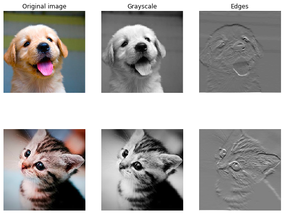
In this code snippet, Python is used to perform simple convolutions. First, imageio and PIL libraries are imported, followed by the two images of a kitten and puppy. After resizing the images, the arrays are stored in array format. In the next step, two filters are applied, one to convert the image to grayscale and the other to detect horizontal edges. In the next step, we apply these filters to the input images using the conv_forward_naive function, and then store the results in the Out variable. The imshow_no_ax function is then defined, which displays images as uint8 and removes axis labels. A side-by-side comparison between the original images and the convolution results is then made using the plt library. The following code snippet shows how to perform a simple convolution operation on images in Python, and how to visualize the results.