Building a Linear Factor Model for Asset Pricing Analysis : Chapter 8

Utilizing Python and Financial Datasets to Estimate Risk and Return Factors

Oct 05, 2024

∙ Paid

This article walks through the process of constructing a linear factor model using Python to analyze asset pricing. The model is based on factors from the Fama-French database and industry portfolio returns, allowing for a deep dive into how different financial variables influence returns. By incorporating various libraries such as pandas, statsmodels, and linearmodels, the analysis efficiently handles data manipulation, regression, and visualization to estimate the risk premia associated with each factor.

The linear factor model helps to uncover the relationships between market returns and risk factors such as size, value, profitability, and investment strategies. This approach is crucial for understanding portfolio performance, guiding investment decisions, and explaining variations in asset returns.

from pprint import pprint
from pandas_datareader.famafrench import get_available_datasets
import pandas as pd
import numpy as np
import matplotlib.pyplot as plt
import seaborn as sns
from statsmodels.api import OLS, add_constant
from pathlib import Path
import warnings
from linearmodels.asset_pricing import TradedFactorModel, LinearFactorModel, LinearFactorModelGMM

This code sets up the environment for building a linear factor model using several libraries. It begins by importing pprint for formatting data structures for better readability, followed by fetching available datasets from Fama/French using get_available_datasets from pandas_datareader, which supplies key financial data for asset pricing models.

Standard libraries such as pandas, numpy, matplotlib, and seaborn are imported for data manipulation, numerical operations, and visualization. Pandas handles data in DataFrame format, while numpy provides efficient array computations. Matplotlib and seaborn are used to create plots for data analysis.

The statsmodels library is included for performing ordinary least squares regression and adding an intercept to the model. Path handling is managed by pathlib.Path for consistency across operating systems. The warnings module is imported to suppress unnecessary warnings in the output.

Lastly, the linearmodels library is incorporated for the TradedFactorModel, LinearFactorModel, and LinearFactorModelGMM classes, which are essential for implementing and estimating the factor model and conducting asset pricing analysis. This code establishes a solid foundation for data handling and analysis in constructing a linear factor model.

Thanks for reading Onepagecode! This post is public so feel free to share it.

# due to https://stackoverflow.com/questions/50394873/import-pandas-datareader-gives-importerror-cannot-import-name-is-list-like
# may become obsolete when fixed
pd.core.common.is_list_like = pd.api.types.is_list_like
import pandas_datareader.data as web

This code addresses an issue with pandas_datareader where the function is_list_like may not be imported correctly, potentially leading to an ImportError. To resolve this, the code redefines is_list_like from the pandas.api.types module to the pd.core.common module, providing a temporary fix for compatibility problems. It then imports the data submodule from pandas_datareader, enabling access to financial datasets for analysis. This allows the retrieval of financial data directly into the Python environment, which is essential for developing and testing the linear factor model in the project. This adjustment ensures the code functions properly without encountering compatibility issues with library versions.

ff_factor = 'F-F_Research_Data_5_Factors_2x3'
ff_factor_data = web.DataReader(ff_factor, 'famafrench', start='2010', end='2017-12')[0]
ff_factor_data.info()

The code retrieves financial data related to a linear factor model from the Fama-French database using the web.DataReader function. The variable ff_factor is assigned the identifier for the ‘F-F_Research_Data_5_Factors_2x3’ dataset, which includes five common factors in asset pricing models: Market risk premium, Size, Value, Profitability, and Investment. The start and end parameters define the data range from January 2010 to December 2017.

Upon execution, the code outputs a summary as a pandas DataFrame with 96 monthly data entries within the specified range. The DataFrame comprises six columns: Mkt-RF, SMB, HML, RMW, CMA, and RF, all containing 96 non-null entries, indicating no missing values. All columns have a float64 data type, suitable for quantitative analysis, and the DataFrame usage is efficient at 5.2 KB. This structured output facilitates further analysis and modeling, providing the necessary factors that influence asset returns in building a linear factor model in finance.

ff_factor_data.describe()

The code snippet ff_factor_data.describe() generates descriptive statistics for a DataFrame in Python that contains financial factor data related to a linear factor model. This function summarizes the central tendency, dispersion, and distribution of the dataset while excluding any NaN values. The output includes key statistics for six columns, which represent different financial metrics: Mk-RF, SMB, HML, RMW, CMA, and RF. Each factor has 96 observations, confirming dataset completeness. The mean values indicate the average return for each factor, with Mk-RF approximately at 1.16, showing a positive average return. The standard deviation values reflect the variability of returns, with Mk-RF exhibiting the highest variability at about 3.58, indicating significant fluctuations.

The minimum and maximum values reveal the range of returns, with Mk-RF showing a minimum of -7.89 and a maximum of 11.35, highlighting a wide performance range. The quartiles provide insights into return distribution, with Mk-RF’s median at approximately 1.24, indicating a right-skewed distribution due to a few high returns elevating the average. This descriptive analysis aids in understanding the characteristics of the financial factors, forming a basis for further analysis or modeling in building a linear factor model. These statistics highlight both average performance and associated risks, which are essential for informed decision-making by investors and analysts.

ff_portfolio = '17_Industry_Portfolios'
ff_portfolio_data = web.DataReader(ff_portfolio, 'famafrench', start='2010', end='2017-12')[0]
ff_portfolio_data = ff_portfolio_data.sub(ff_factor_data.RF, axis=0)
ff_portfolio_data.info()

The code retrieves financial data from the Fama-French database, specifically the 17 Industry Portfolios dataset, using the web.DataReader function for the period from January 2010 to December 2017. It adjusts the portfolio returns by subtracting the risk-free rate, allowing for an analysis of excess returns compared to risk-free investments. The resulting DataFrame contains 96 monthly entries and is structured as a PeriodIndex, indicating monthly organization. There are 17 columns representing various industry sectors, with each column containing 96 non-null float64 values, confirming no missing data points. The DataFrame has a memory usage of 13.5 KB, which is efficient for this dataset. This output validates that the data is well-organized and complete, making it reliable for further financial modeling and analysis, such as constructing a linear factor model.

ff_portfolio_data.describe()

The code snippet ff_portfolio_data.describe() generates descriptive statistics for a DataFrame in Python using the pandas library. This function summarizes the central tendency, dispersion, and distribution shape of the dataset, excluding NaN values. The output includes several important statistics for each column, such as the count of non-null entries, mean, standard deviation, minimum, maximum, and quartiles.

For instance, the Food column has a mean of approximately 1.05 and a standard deviation of about 1.51, indicating the average value and variability of the data. The minimum value for this column is -5.17, and the maximum is 6.67, suggesting significant data variation. Similar statistics apply to other columns like Mines, Oil, and Clths. The Mines column has a mean of 0.20 and a standard deviation of 0.55, indicating a low average with some variability. The quartiles provide additional insight into data distribution, with the 25th percentile for Cars at -1.25 and the 75th percentile at 4.80, showing half of the data points fall within this range.

Overall, the descriptive statistics from describe() are essential for understanding the dataset’s characteristics and support further analysis and modeling, such as building a linear factor model. This summary aids in identifying trends, outliers, and data distribution, which are vital for informed financial modeling and analysis decisions.

with pd.HDFStore('../../data/assets.h5') as store:
    prices = store['/quandl/wiki/prices'].adj_close.unstack().loc['2010':'2017']
    equities = store['/us_equities/stocks'].drop_duplicates()

This code snippet utilizes the Pandas library to manage data in HDF5 format. It opens the HDF5 file named assets.h5, located two directories up from the current working directory. Within the file, it accesses two datasets. The first dataset contains adjusted closing prices of assets from the Quandl database. By using store[‘/quandl/wiki/prices’].adj_close.unstack(), it retrieves and transforms the adjusted closing prices into a flat structure, filtering the rows to include only data from 2010 to 2017. This results in a table of adjusted closing prices for each asset across those years. The second dataset consists of U.S. equities, accessed via store[‘/us_equities/stocks’]. The drop_duplicates() method is applied to remove any duplicate entries. Consequently, there are two structured datasets: one with price information for the specified years and another with a clean list of equities.

sectors = equities.filter(prices.columns, axis=0).sector.to_dict()
prices = prices.filter(sectors.keys()).dropna(how='all', axis=1)

This code snippet works with two data structures, equities and prices. It first extracts the sectors for each equity in the equities DataFrame by using the filter method to select relevant columns based on the index labels in prices. The code then accesses the sector attribute and converts the resulting series into a dictionary, mapping equity identifiers to their corresponding sector assignments.

Next, the code processes the prices DataFrame by again using the filter method to retain only the columns that match the equity tickers in the sectors dictionary. This filtering removes any irrelevant columns, followed by a dropna method call that removes columns from prices containing only NaN values. The result is a cleaned prices DataFrame that includes only the equities in relevant sectors and eliminates any columns lacking price data.

returns = prices.resample('M').last().pct_change().mul(100).to_period('M')
returns = returns.dropna(how='all').dropna(axis=1)
returns.info()

The code processes a DataFrame containing price data, transforming it to analyze returns over time. It resamples the data on a monthly basis, capturing the last price of each month, which is essential for calculating monthly returns. The percentage change in prices is then calculated, representing the difference between the current month’s price and the previous month’s price as a percentage. The index is converted to a monthly period format for clarity.

After calculating the returns, the code cleans the DataFrame by dropping rows and columns that contain only NaN values, ensuring a clean dataset for analysis. The resulting DataFrame has 95 entries, covering the period from February 2010 to December 2017, with a monthly frequency. It includes 1,936 entries across multiple columns, indicating various assets or factors under analysis. The data is stored as floating-point numbers, which is standard for financial data, and the overall memory usage is 1.4 MB, making it manageable for further analysis. This approach to calculating and organizing returns is foundational for developing a linear factor model to understand asset performance over time.

ff_factor_data = ff_factor_data.loc[returns.index]
ff_portfolio_data = ff_portfolio_data.loc[returns.index]

This code filters the ff_factor_data and ff_portfolio_data DataFrames to include only the rows with indices present in the returns DataFrame, aligning the datasets with available return data. By slicing both DataFrames with the index from the returns DataFrame, entries that do not match are removed. This results in cleaner DataFrames better suited for subsequent analysis related to returns, ensuring that any future computations or model fittings align with the time periods of the returns data and avoid misalignment issues.

ff_factor_data.describe()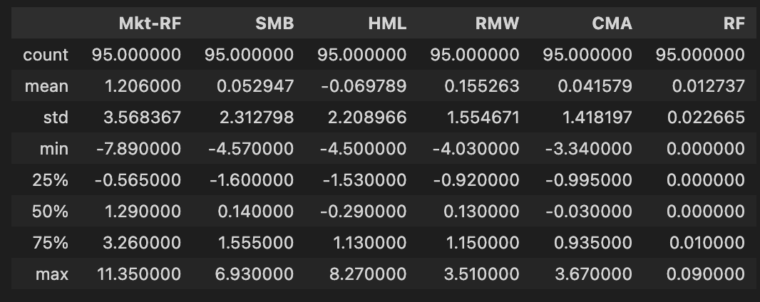

The code snippet ff_factor_data.describe() generates descriptive statistics for a DataFrame in Python that contains financial factor data related to a linear factor model. It summarizes key aspects of the dataset’s distribution, excluding NaN values. The output includes statistics for five columns: Mk-RF, SMB, HML, RMW, CMA, and RF, with 95 observations for each factor, indicating dataset completeness. The mean values reveal that Mk-RF has an average of approximately 1.206, indicative of a positive average excess return over the risk-free rate, while the other factors have means close to zero, signaling relatively neutral average returns.

Standard deviation values indicate variability, with Mk-RF showing about 3.568, reflecting significant fluctuations in its returns. In contrast, SMB and HML exhibit lower standard deviations, suggesting more stable performances. The range of returns is highlighted by the minimum and maximum values, with Mk-RF ranging from -7.89 to 11.35, suggesting potential for substantial losses and gains. Percentile values further illustrate data distribution, with the median of Mk-RF at 1.29, higher than those of the other factors, emphasizing its stronger performance.

This descriptive analysis is essential for understanding the behavior of the factors in the linear model, aiding researchers and analysts in assessing risk and return characteristics necessary for informed investment decisions.

excess_returns = returns.sub(ff_factor_data.RF, axis=0)
excess_returns.info()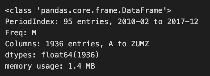

The code calculates excess returns by subtracting the risk-free rate from a DataFrame of returns using the sub method from the pandas library for element-wise subtraction. The risk-free rate data is aligned with the returns data by their indices, ensuring accurate subtraction for each entry.

The output of the excess_returns.info() method summarizes the resulting DataFrame, which is a two-dimensional structure with an index ranging from February 2010 to December 2017 and containing 95 entries organized monthly. It has 1,936 columns, representing different assets or factors involved in the analysis.

Entries are specified as float64, indicating that values are stored as 64-bit floating-point numbers, suitable for financial data with decimal values. The DataFrame uses 1.4 MB of memory, reflecting the resource requirements for processing. This code snippet and its output are essential for establishing a linear factor model, forming the basis for analyzing asset performance relative to the risk-free rate.

excess_returns = excess_returns.clip(lower=np.percentile(excess_returns, 1),
                                     upper=np.percentile(excess_returns, 99))

This code adjusts the excess_returns data to limit extreme values by using the clip method to constrain it within specific thresholds. It sets a lower bound at the 1st percentile and an upper bound at the 99th percentile. Any values below the 1st percentile are replaced with the 1st percentile value, and any values above the 99th percentile are replaced with the 99th percentile value. This clipping reduces the impact of outliers on the dataset, allowing for a more accurate analysis of performance by focusing on the central range of values.

ff_portfolio_data.info()

The method call ff_portfolio_data.info() is part of the Pandas library in Python and summarizes a DataFrame named ff_portfolio_data, which contains financial data related to a linear factor model. The output shows that ff_portfolio_data is a Pandas DataFrame with 95 entries, indicating 95 rows of data for specific time periods. The index is a PeriodIndex that spans from February 2010 to December 2017, with monthly frequency, which is relevant for time series analysis often used in financial modeling.

The DataFrame has 17 columns, each representing different financial variables or factors, with names such as Food, Oil, Mines, and Cnsum. All columns contain 95 non-null entries of type float64, confirming that all values are numeric and there are no missing entries, which is important for the integrity of data analysis.

Its memory usage is reported as 15.9 KB, indicating that the dataset is relatively small and manageable. The presence of 17 data types, all being float64, suggests the data is continuous and suitable for quantitative analysis like regression modeling. This summary offers a clear overview of the dataset’s structure, which is essential for any subsequent analysis in building a linear factor model.

ff_factor_data.info()

The code ff_factor_data.info() displays a summary of a DataFrame in pandas, a widely used data manipulation library in Python. This DataFrame, ff_factor_data, likely contains financial factor data related to the Fama-French model, which explains stock returns.

The output indicates that the DataFrame is of type pandas.core.frame.DataFrame and contains 95 entries, covering a time frame from February 2010 to December 2017 with monthly data frequency. It lists several columns representing essential factors in the Fama-French model, including Mkt-RF, SMB, HML, RMW, CMA, and RF. Each of these columns contains 95 non-null entries of data type float64, indicating numerical values for returns or factors. The total memory usage is 5.2 KB, providing insight into the dataset’s size.

This output offers a clear overview of the structure and contents of the ff_factor_data DataFrame, making it suitable for financial analysis or modeling using this data. Understanding this structure is important for those involved in financial analysis.

betas = []
for industry in ff_portfolio_data:
    step1 = OLS(endog=ff_portfolio_data.loc[ff_factor_data.index, industry], 
                exog=add_constant(ff_factor_data)).fit()
    betas.append(step1.params.drop('const'))

This code snippet calculates betas for various industries using a linear regression model based on the ordinary least squares method. It initializes an empty list to store the regression coefficients for each industry and iterates through each industry in ff_portfolio_data. For each industry, it performs regression analysis where the endogenous variable is the industry’s returns matched with the indices from ff_factor_data. The independent variables consist of factors from ff_factor_data, including a constant term for the regression intercept. After fitting the model, it extracts the parameters while removing the constant term and appends the resulting betas, which indicate the sensitivity of the industry’s returns to the factors, to the list. The final output is a list of betas for each industry for further analysis or modeling tasks.

Thanks for reading Onepagecode! This post is public so feel free to share it.

betas = pd.DataFrame(betas, 
                     columns=ff_factor_data.columns, 
                     index=ff_portfolio_data.columns)
betas.info()

The code creates a Pandas DataFrame named betas that organizes beta coefficients from a linear factor model. It uses the betas variable for construction, with columns representing factors from ff_factor_data and the index set to portfolios from ff_portfolio_data. This setup clearly shows how portfolio returns are influenced by various factors.

The output of the betas.info method summarizes the DataFrame’s structure, indicating it contains 17 entries, likely representing different portfolios or assets, and 6 columns for the model’s factors, which include market return minus risk-free rate, small minus big, high minus low, robust minus weak, conservative minus aggressive, and risk-free rate. These factors are essential for understanding the risk and return characteristics of the portfolios.

Additionally, the output confirms that all entries are non-null, indicating there are no missing values, which is crucial for accurate analysis. The columns are all float64 data types, meaning the values are numerical and suitable for mathematical operations. The DataFrame has a memory usage of 1.6 KB, indicating a manageable dataset size. Overall, this code offers a structured view of the relationship between portfolios and factors, which is fundamental for analyzing performance and risk in the context of the linear factor model.

lambdas = []
for period in ff_portfolio_data.index:
    step2 = OLS(endog=ff_portfolio_data.loc[period, betas.index], 
                exog=betas).fit()
    lambdas.append(step2.params)

This code snippet estimates the factor loadings, known as lambdas, from portfolio returns over various periods. It initializes an empty list called lambdas and iterates through each period in the ff_portfolio_data DataFrame index. For each period, it fits an Ordinary Least Squares regression model. The dependent variable, endog, represents the portfolio returns for that period, accessed via ff_portfolio_data.loc[period, betas.index]. The independent variables, exog, consist of the factors defined in the betas DataFrame. After fitting the model, the resulting parameters, including the estimated lambdas, are appended to the lambdas list. By the end of the loop, all estimated lambdas for each period are accumulated for further analysis of the relationship between the factors and asset returns.

lambdas = pd.DataFrame(lambdas, 
                       index=ff_portfolio_data.index,
                       columns=betas.columns.tolist())
lambdas.info()

The code snippet creates a Pandas DataFrame named lambdas to store data related to a linear factor model. It is initialized with values representing the estimated factor loadings of a portfolio to various risk factors. The index of this DataFrame aligns with the index of ff_portfolio_data to ensure proper time series consistency. The columns are based on the names from the betas DataFrame, which contains the names of the analyzed factors.

The output of the lambdas.info() method summarizes the DataFrame’s structure, showing 95 entries of monthly data from February 2010 to December 2017, with a monthly frequency. There are six columns representing different factors: Mkt-RF, SMB, HML, RMW, CMA, and RF. Each column contains 95 non-null float64 values, confirming there are no missing data points. The DataFrame uses 7.7 KB of memory, indicating efficient data storage.

This structure is crucial for analyzing the contributions of different factors to portfolio returns, enabling a better understanding of associated risk exposures. The alignment of indices and completeness of data allow for seamless subsequent analyses, such as regression modeling or performance evaluation, without concerns related to missing values or misaligned time series.

lambdas.mean()

The code snippet lambdas.mean() calculates the mean of values stored in the variable lambdas, which likely includes estimated coefficients from a linear factor model used in finance to explain asset returns based on risk factors. The output presents mean values for factors such as Mkt-RF, SMB, HML, RMW, CMA, and RF.

Mkt-RF, representing the market risk premium, indicates a strong expectation that the market will outperform the risk-free rate with a value of 1.244610. The SMB factor has a mean of 0.007380, showing a slight positive return associated with small-cap stocks compared to large-cap stocks, although this effect is minimal. The HML factor, with a mean of -0.696972, suggests value stocks are underperforming growth stocks. The RMW factor, at -0.265768, indicates that firms with strong profitability are underperforming those with weak profitability. Similarly, the CMA factor shows a mean of -0.308635, pointing to lower returns from conservative investment strategies compared to aggressive ones. Lastly, the RF value of -0.013344 suggests a negative risk-free rate, which may reflect unusual market conditions. The values are stored as float64, ensuring high precision in calculations. This output summarizes the relationships between market returns and various risk factors in the linear factor model.

t = lambdas.mean().div(lambdas.std())
t

The code snippet calculates a standardized measure of the mean of a dataset represented by lambdas by dividing the mean of the lambdas values by their standard deviation. This results in a variable t that indicates how many standard deviations the mean is from zero. The output presents the standardized means for several factors, including Mkt-RF, SMB, HML, RMW, CMA, and RF, each accompanied by a value. For example, Mkt-RF has a value of approximately 0.347, indicating that its mean is about 0.347 standard deviations above zero, while RF is approximately -0.160, suggesting its mean is 0.160 standard deviations below zero. These standardized values are beneficial in a linear factor model, as they enable the comparison of different factors on a common scale, making it easier to assess their relative influence in the model. The output values are stored as floating-point numbers, standard for numerical computations in Python. This code snippet and its output provide insights into the behavior of various financial factors, enhancing understanding of their relationships in the model.

ax1 = plt.subplot2grid((1, 3), (0, 0))
ax2 = plt.subplot2grid((1, 3), (0, 1), colspan=2)
lambdas.mean().plot.barh(ax=ax1)
lambdas.rolling(60).mean().plot(lw=2, figsize=(14,10), sharey=True, ax=ax2);

The code snippet uses Matplotlib to create a visual representation of financial data centered on a linear factor model. It features two subplots: the first subplot displays a horizontal bar chart showing the mean values of various factors, and the second subplot presents a line plot of the rolling mean of these factors over time.

Building a Linear Factor Model for Asset Pricing Analysis : Chapter 8

Utilizing Python and Financial Datasets to Estimate Risk and Return Factors

This post is for paid subscribers