Building a Robust LSTM Stock Price Prediction Pipeline: Overcoming Overfitting and Normalization Bias

A complete walk-through on building a reliable forecasting pipeline, fixing common normalization errors, and comparing simple baselines on historical GE stock data.

Onepagecode

May 28, 2026

∙ Paid

Download the entire source code using the button at the end of this article.

Overfitting that stems from having too little effective data.

Excessive and unnecessary feature engineering that likely increased noise.

Incorrect choice of normalization that led to poor predictions.

Lack of systematic hyperparameter tuning.

Note: instead of directly forecasting raw prices, the project focuses on predicting price movement (average of high and low), since LSTM models often perform better at learning directional or smoothed signals than noisy raw quotes.

What this notebook will do (high-level steps)

Acquire historical price data and prepare the Colab environment.

Visualize the price series to understand the signal.

Apply a more appropriate normalization strategy to the data.

Explore simple baselines such as moving averages and exponential moving averages for one-step-ahead prediction.

Tune model hyperparameters and compare configurations.

Compute a daily average price from high and low, then split the series into training and test sets.

Train a multilayer LSTM network on the prepared data.

Plot model outputs alongside the reference series for qualitative comparison.

Run experiments varying hyperparameters and training settings to detect overfitting or underfitting.

Summarize findings and draw conclusions.

Part 1 — Prepare the Google Colab environment

This section gets the Colab runtime ready for the notebook: mount Google Drive, verify that a GPU is present, and import the Python packages and libraries needed for the rest of the analysis.

#import libraries
from pandas_datareader import data
import matplotlib.pyplot as plt
import pandas as pd
import datetime as dt
import urllib.request, json 
import os
import numpy as np
import tensorflow as tf 
from sklearn.preprocessing import MinMaxScaler

The cell pulls together the Python libraries the rest of the notebook will rely on, so that data acquisition, manipulation, plotting, numerical work, model building, and preprocessing utilities are available under convenient names. Importing a module loads its code into the interpreter and binds it to a local name or alias, making functions and classes from that library callable in later cells.

The data reader module provides helpers to fetch financial time series from online sources and return them as tabular objects; the plotting library gives access to a stateful plotting interface for visualization; the data frame library offers efficient tabular structures and I/O for CSVs and similar files; the datetime module helps create and manipulate date objects for indexing and slicing time series. The urllib and json modules are present to make HTTP requests and parse JSON responses when needed, while the operating-system interface lets the notebook inspect or construct file paths. The numerical array library supplies fast array storage and vectorized operations used throughout preprocessing and model input construction, and the machine-learning framework provides the computational graph, tensor operations, and training primitives for building and fitting the LSTM. Finally, the scaler from the preprocessing subpackage will be used to map raw price values into a stable numeric range for training.

There is no printed output from running these imports, which simply prepares the environment; any messages that sometimes appear (library version warnings or device initialization logs) are not present here, so the cell’s effect is limited to making these modules available under the chosen aliases for use by later steps.

#declare name of your device and drive location select GPU
device_name = tf.test.gpu_device_name()
if device_name != '/device:GPU:0':
  raise SystemError('GPU device not found')
print('Found GPU at: {}'.format(device_name))

Found GPU at: /device:GPU:0

Its purpose is to make sure TensorFlow can see and use a GPU before the notebook proceeds to GPU-dependent work. The cell asks TensorFlow for the name of the GPU device it detects, compares that result to the expected device path for the primary GPU, and halts execution with a clear error if no suitable GPU is found. Doing this early prevents later code from running under the wrong assumptions (for example, trying to allocate large models on CPU and failing or being extremely slow) and gives an explicit, easy-to-understand failure mode instead of a cascade of obscure errors.

The printed confirmation shown in the saved output, "Found GPU at: /device:GPU:0", indicates that TensorFlow reported the primary GPU device and the check succeeded. The specific path denotes GPU number zero in the runtime; it tells you that the environment exposes at least one GPU and that subsequent TensorFlow operations can target it. If the check had failed, the notebook would have raised an error and stopped, but because the message appears, the rest of the GPU-accelerated training and model work can proceed with confidence.

from google.colab import drive
drive.mount("/content/drive", force_remount=True)

Mounted at /content/drive

The cell establishes a connection between the Colab runtime and the user's Google Drive so files stored in Drive become part of the notebook's filesystem and can be read from or written to by later cells. Behind the scenes Colab runs an authentication and mount routine that grants the session access to the Drive contents and exposes them at a standard mount point inside the container.

The mount was requested with a force-remount behavior, which refreshes the mount even if Drive was already mounted in this session; that is helpful when rerunning cells or when a previous mount may be stale. The printed message "Mounted at /content/drive" in the saved output confirms the operation succeeded and that the Drive contents are now available under that path. Subsequent cells can therefore reference files inside the Drive (for example the notebook's dataset) using paths beneath that mount point; if mounting had failed you would instead see an authentication prompt or an error rather than this confirmation.

Choosing General Electric (GE) as the dataset instead of Amazon

I switched to GE because its historical record gives more observations over a longer span, which makes it easier to study extended trends. Amazon’s recent rapid growth covers only a few years, so the available daily records are relatively concentrated and make it harder to align training and test periods for this experiment.

For example, if the model requires around nine hundred samples for training and we reserve roughly one hundred eighty days for testing, that consumes a substantial portion of the shorter Amazon history. Amazon’s major rise is concentrated in about four years of trading days, which is only around twelve hundred daily points in total, so there is less room to hold out test data while still having a robust training set for one-day-ahead and pattern-based forecasting.

With GE’s larger series we have more headroom to split the data without starving the model, which reduces concerns about overfitting and lets us concentrate on improving the training procedure.

#name of your google path
googlepath = "/content/drive/My Drive"

A variable is assigned the standard Colab Google Drive mount path (/content/drive/My Drive) so later file operations can build full filesystem paths by joining that base location with filenames. Storing the drive root in a single variable makes the rest of the notebook cleaner and easier to adjust if the mount point changes or if you want to run the notebook in a different environment.

There is no visible output from this step because it only creates an in-memory string and does not perform any file I/O or validation. Before attempting to read or write files using that path, the Drive must be mounted in the runtime; otherwise subsequent file access calls that rely on this variable will fail because the directory does not exist.

#Get your API data
df = pd.read_csv(os.path.join(f'{googlepath}','ge.us.txt'),delimiter=',',usecols=['Date','Open','High','Low','Close'])

It reads the CSV file named ge.us.txt from the Google Drive path and loads the selected columns into a pandas DataFrame assigned to the variable df. The file path is constructed with a path-joining call so the filename is combined with the previously defined googlepath; the read function is told explicitly that values are comma-separated and to keep only the Date, Open, High, Low and Close columns, which reduces memory and parsing work by ignoring any other columns in the file.

Behind the scenes pandas opens and parses the file, infers numeric types for the price columns and leaves the Date values as strings unless a date-parsing option is supplied. If the file is not present at the given location or cannot be opened, pandas will raise an error at this step. There is no printed or displayed output saved from this cell; the effect is to prepare and store the loaded table in df so subsequent cells can compute averages, split train/test, and run further processing.

df = df.sort_values('Date')
df.head()

         Date     Open     High      Low    Close
0  1970-01-02  0.30627  0.30627  0.30627  0.30627
1  1970-01-05  0.30627  0.31768  0.30627  0.31385
2  1970-01-06  0.31385  0.31385  0.30996  0.30996
3  1970-01-07  0.31385  0.31385  0.31385  0.31385
4  1970-01-08  0.31385  0.31768  0.31385  0.31385

The DataFrame has been ordered by the Date column so the rows follow chronological order, and then the first five rows are shown to give a quick sanity check. Sorting by Date with the default ascending option places the earliest timestamps at the top, and because the dates are in ISO format (YYYY-MM-DD) a lexicographic sort produces the same chronological order whether the Date column is a string or a datetime type. Note that sorting does not automatically change the row labels, so the original index values are preserved rather than being reset to 0, 1, 2, …

The printed table shows the earliest five trading days: 1970-01-02 through 1970-01-08, with the usual OHLC columns. The numeric values are small decimals (for example 0.30627), and you can see cases where Open, High, Low and Close are identical on a day, which simply means there was no intra-day price movement recorded at the precision shown. On 1970-01-05 the High is larger (0.31768), illustrating a one-day uptick compared with neighboring rows.

Jupyter provides both a plain-text and an HTML tabular representation of the output; the head display is useful here to confirm that sorting had the intended effect and to inspect the earliest records for any obvious anomalies. Ensuring the rows are in chronological order is important for subsequent time-series computations such as windowed scaling, moving averages, or sequential model training.

Compute the per-day midpoint of High and Low prices and display the resulting time series

plt.figure(figsize = (18,9))
plt.plot(range(df.shape[0]),(df['Low']+df['High'])/2.0)
plt.xticks(range(0,df.shape[0],500),df['Date'].loc[::500],rotation=45)
plt.xlabel('Date',fontsize=18)
plt.ylabel('avg Price',fontsize=18)
plt.show()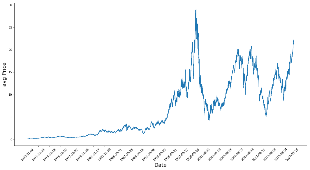

The figure plots a single time series built from the average of the daily High and Low prices, so each point represents the midpoint of that day's trading range rather than a single price like Close. Using the midpoint smooths out some of the intraday bid-ask spread noise and gives a clearer view of the underlying longer-term price movement.

To keep the plot readable for a long history, the x-axis shows only every 500th date label and those labels are rotated so they don't overlap; the axes are labeled so you know the horizontal axis is calendar Date and the vertical axis is the average price. The plot itself is drawn at a wide aspect ratio so the daily fluctuations form a continuous, dense line rather than individual dots, making trends and regime changes easy to see.

The saved output shows what you would expect from that procedure: the series starts at very low values, rises gradually for many years, then exhibits a very large spike followed by a sharp decline and then several large oscillations. That dramatic peak and collapse are immediately visible because the y-axis is scaled to include the peak, which makes smaller fluctuations earlier in the history appear relatively muted. The dense trace near the end of the plot reflects many closely spaced daily samples, and the sampled x-tick labels explain the rotated date strings you see along the bottom. The notebook's textual figure summary confirms a single figure object with one axes and the full image is attached as the visual output.

Viewed from a modeling perspective, this visualization highlights non-stationarity and multi-scale volatility in the series: long periods of slow growth, sudden large moves, and later high-amplitude oscillations. Those features explain why it’s useful to apply careful normalization and smoothing before training predictive models, and why any baseline or LSTM will need to handle both gradual trends and abrupt shifts.

# First calculate the average prices from the highest and lowest 
high_prices = df.loc[:,'High'].as_matrix()
low_prices = df.loc[:,'Low'].as_matrix()
avg_prices = (high_prices+low_prices)/2.0

/usr/local/lib/python3.6/dist-packages/ipykernel_launcher.py:1: FutureWarning: Method .as_matrix will be removed in a future version. Use .values instead.
  """Entry point for launching an IPython kernel.
/usr/local/lib/python3.6/dist-packages/ipykernel_launcher.py:2: FutureWarning: Method .as_matrix will be removed in a future version. Use .values instead.

The three lines extract the per-row high and low prices from the DataFrame and convert them into plain numeric arrays, then compute a simple central price for each day by averaging the high and low. Converting the DataFrame columns to arrays gives two one-dimensional NumPy arrays of the same length, the element-wise addition produces a new array of summed highs and lows, and dividing by two yields a floating-point array named avg_prices that holds the daily midpoint price for every row; that array is what later plotting, normalization, and modeling steps will consume.

The printed messages are FutureWarning notices emitted because the column-to-array conversion used a deprecated pandas method; the operation still succeeded, but pandas is telling you that asmatrix will be removed and that the modern alternative is to use the .values attribute. Functionally nothing else changed by these warnings: the arrays were created and avgprices computed, but to future-proof the notebook you should replace the deprecated call with the recommended approach.

Observations from the plot

The price series shows a peak near 1983, followed by an overall upward trend that is interrupted by two major declines: one occurring around 2001 (close to the events of September 11) and another during the period of the 2009 financial market crash. These drops are clearly visible in the long-term trace.

Representing each day by the average of the High and Low reduces short-term volatility and yields a clearer view of daily behavior than looking at High or Close values alone. The averaged series better captures activity across the entire trading day rather than a single moment.

The dataset comprises roughly twelve thousand records.

The series is partitioned so that the first eleven thousand records form the training set and the remainder is reserved for testing.

The training portion is normalized before any downstream processing.

train = avg_prices[:11000]
test = avg_prices[11000:]
len(avg_prices)

Two simple assignments carve the average-price series into a training segment and a test segment by slicing the sequence at index 11,000. The slice that becomes the training set takes every entry from the start up to, but not including, index 11,000, so it contains the chronologically earlier 11,000 observations. The test set takes every entry from index 11,000 to the end, so it contains the later observations that will be held out for evaluation; because Python slicing uses a zero-based index and an exclusive end bound, the split cleanly separates the first 11,000 points from the remainder.

The length query that follows reports the total number of observations in the full series; the saved output shows 12,075, which means the held-out test portion contains 12,075 minus 11,000, or 1,075, observations. Because the split is chronological rather than random, the training data represents earlier history and the test data represents later unseen periods, which is the appropriate arrangement for time-series forecasting to avoid look-ahead bias.

Normalize the series by scaling it

What we'll do

Break the full price sequence into consecutive blocks and scale each block independently.
For example, using a block length of 2500 on a series of 10000 points will produce four separate blocks to normalize.
Any leftover samples at the end are handled by fitting and applying the scaler to that final fragment.
Use a MinMaxScaler so that transformed values fall between zero and one.

Note: before fitting the scaler, reshape the train and test arrays into a column shape (number of samples by one feature) so scikit-learn expects the correct input dimensions.

Why use windowed scaling

Market data has changing amplitude over time. If you fit a single global scaler to the entire historical series, early periods with much smaller values can be compressed near zero and contribute little to model learning. By normalizing each time window separately, each segment keeps useful dynamic range for training. In this notebook we use a window size of 2500 for that reason.

scaler = MinMaxScaler() #use mimaxscaler from scikitlearn to normalize data
train = train.reshape(-1,1)
test = test.reshape(-1,1)

The cell prepares the normalization tools and the data shape that the scaler expects. A MinMaxScaler object is created so that later numerical values can be rescaled into a fixed range, and both the training and test arrays are converted from one-dimensional sequences into two-dimensional column arrays with shape (numberofsamples, 1).

Behind the scenes, scikit‑learn’s transformers require a 2D array where rows are samples and columns are features; reshaping with a single column satisfies that requirement. Instantiating the scaler does not yet compute any statistics — it only constructs the scaler object — and the reshape operation simply changes the arrays’ view/shape in memory so subsequent fit or transform calls will accept them. There is no printed output from these assignments, so nothing appears in the saved output.

Normalize the average-price series and forecast it directly rather than creating many engineered features

The dataset contains roughly 12,075 daily observations. Instead of expanding the input with numerous derived indicators, we will work directly with the per-day average price and prepare that series for modeling by applying a sliding-window normalization scheme. This keeps the input simple and stabilizes the scale across time before training predictive models.

window_size = 2500
for x in range(0,10000,window_size):
    scaler.fit(train[x:x+window_size,:])
    train[x:x+window_size,:] = scaler.transform(train[x:x+window_size,:])

scaler.fit(train[x+window_size:,:])
train[x+window_size:,:] = scaler.transform(train[x+window_size:,:])

A sliding-window MinMax normalization is applied to the training series using a window length of 2,500 samples. The loop steps through the training array in non-overlapping blocks and, for each block, fits the scaler to that block’s values and immediately replaces the block with its scaled version. Because the loop variable remains set to the last iterated start index after the loop finishes, an extra fit/transform call follows that operates on whatever portion of the training array remains after the final full window; that final fit leaves the scaler object configured to the last chunk processed.

Behind the scenes, each fit computes the minimum and maximum for the single feature column in that block, and each transform linearly rescales values into the 0–1 range relative to that block’s min and max. The net effect is that training values are normalized locally within each time window rather than globally across the entire training set, which adapts scaling to changing ranges over time and avoids using future data to rescale earlier samples. There is no printed or returned output from this cell; the visible result is the in-memory replacement of the training array with its per-window scaled values and a scaler instance fitted to the final chunk that can be used later to transform other data.

# Reshape both train and test data
train = train.reshape(-1)

The single operation converts the train array into a one-dimensional sequence by collapsing any existing extra dimension into a flat vector. Using a reshape parameter of -1 tells NumPy to compute the appropriate length automatically so the result contains the same number of elements but as a 1-D array instead of a column or 2-D structure.

No printed output is produced by this reassignment; the cell simply prepares the train data for subsequent steps where a flat sequence is easier to index, iterate over, or pass to functions that expect a one-dimensional input. Making train a 1-D array avoids extra indexing like [:,0] later and ensures downstream code that treats the series as a simple sequence will work as intended.

Convert the input into a two-dimensional array suitable for training

# Normalize test data
test = scaler.transform(test).reshape(-1)

The previously fitted scaler is applied to the test series so the test values are expressed on the same normalized scale that the model and any baseline calculations expect. Behind the scenes the scaler uses the min and max (or whatever parameters it learned during fitting) to linearly rescale each test sample, so values that were at the training minimum map near the lower bound and values at the training maximum map near the upper bound; values outside the training range will be mapped outside the usual 0–1 interval because the transform is a linear extrapolation based on the fitted parameters.

The transformed data is then flattened into a one-dimensional array: the scaler treats inputs and outputs as two-dimensional column vectors (samples by features), so the reshape step removes that single-feature column dimension to produce a simple sequence vector that downstream code can index and iterate over. Because the result is assigned back to the test variable, subsequent operations in the notebook will see the normalized test series rather than the original raw values. There is no printed or displayed output from this operation because it only performs an in-memory assignment; to inspect the result one would need an explicit display or print after the transformation.

Note that the test partition is not refit with a new scaler. Instead, the scaler trained on the final training window is applied to the test set and the transformed values are reshaped to match the training data layout. In other words, we do not refit the normalization on test data; we only transform it with the scaler obtained from training.

After normalization you can apply exponential moving average smoothing to reduce short-term jitter in the price series. This smoothing operation produces a cleaner trend line by dampening the high-frequency fluctuations that are typical in intraday and daily stock price data.

Important: perform the EMA smoothing only on the training data. Do not smooth the test set.

Reference: https://datascience.stackexchange.com/questions/27615/should-we-apply-normalization-to-test-data-as-well

Smoothing with an exponential moving average

EMA = 0.0 # keep EMA 0.0
ema2 = 0.1 # gamma is a variabe that can be multiplied with train 
for i in range(11000):
  EMA = ema2*train[i] + (1-ema2)*EMA
  train[i] = EMA

An exponential moving average filter is being applied across the first 11,000 entries of the training series to smooth short-term fluctuations. The smoothing state is stored in a single scalar named EMA that starts at zero, and the smoothing factor (alpha) is set to 0.1. For each index from 0 up to 10,999 the scalar EMA is updated to a weighted blend of the current recorded value at that index and the previous EMA: the new EMA is 10% of the current raw value plus 90% of the previous EMA. After computing that blended value it overwrites the training series at the same index with the EMA value, so the stored sequence becomes the running exponential average up to that point.

Because EMA begins at zero, the very first updated entry becomes 0.1 times the original first value, which slightly biases the start downward compared with initializing EMA to the first data point; subsequent steps quickly ramp the EMA toward the series’ level. Using alpha = 0.1 makes the filter relatively sluggish: it smooths out fast spikes and high-frequency noise but introduces a short lag behind sudden changes. The filter is applied in place only to those first 11,000 samples, so after this loop the training array has been permanently replaced by its smoothed version while later entries remain unchanged. There is no printed or plotted output from this cell; its effect is the modified, smoothed training data that later code will use.

# Used for visualization and test purposes
all_avg_data = np.concatenate([train,test],axis=0)

The cell produces a single continuous time series called allavgdata by joining the preprocessed training and testing arrays end-to-end. Behind the scenes, the array-concatenation routine allocates a new NumPy array large enough to hold both pieces and copies the training rows first, then the testing rows, so the original chronological order is preserved. Because the inputs being joined were already prepared (scaled and smoothed as appropriate earlier), the resulting array contains the exact values you want to use for plotting and for aligning model predictions with the true series.

There is no printed output from this assignment; the effect is to create and store the allavgdata variable in the session namespace so later cells can index, slice, plot, or compute errors against the full series. Notice that concatenation duplicates the data into a new buffer, so it uses additional memory equal to the sum of the two parts, but it simplifies downstream operations by keeping a single array that spans both train and test periods.

One-Step-Ahead Forecasts Using Average-Based Baselines

In this section we build straightforward reference models that predict the next time-step by summarizing recent values. Two variants are tested: a simple moving average computed over a fixed window of past observations, and an exponential moving average that assigns greater weight to more recent points. For each method we produce one-step-ahead predictions, evaluate their mean squared error on the held-out portion of the series, and visualize the predicted sequence alongside the true average-price series.

What is one-step-ahead prediction?

One-step-ahead forecasting means using past observations of a time series to produce a single prediction for the next time point. In practice this task asks: given the history up to today, what will tomorrow look like?

How we apply it here

We reduce each trading day to a single value by averaging the day's High and Low prices. The goal is to train a model on these historical daily averages so it can output a predicted value for the following day. Once trained, the same procedure can be repeated to continue generating one-day-ahead forecasts for as long as desired.

Simple averaging baselines

A straightforward way to guess the next value is to summarize recent observations and use that summary as the prediction. Two common approaches of this kind are:

a simple moving average computed over a fixed recent window of days, and
an exponential moving average that weights recent days more heavily than older ones.

These methods are easy to compute but tend to lose accuracy when extended to predict many steps into the future. In this notebook we compare both visually (by plotting predictions against the true series) and numerically using an error metric.

How we measure error

We quantify forecast quality with mean squared error. For each one-step-ahead prediction, we take the difference between the true next-day value and the predicted value, square that difference, and then average those squared values across all predictions. This average provides a single number summarizing how far the predictions deviate from the truth.

Simple Averaging:

Start with a very basic approach to gauge how hard the forecasting task is: predict the next data point by taking an average of a fixed number of recent observations. For example, to estimate tomorrow's price you might compute the arithmetic mean of the last one hundred days of observed average prices. After testing this straightforward moving-window mean, we will try a slightly more sophisticated baseline that weights recent observations more heavily using an exponential moving average. These two simple strategies provide a point of comparison before moving on to a recurrent neural network solution based on Long Short-Term Memory units, which aims to learn more complex temporal patterns.

Concretely, the simple baseline uses the mean of the values inside the chosen window as the forecast for the following day. The exponential moving average baseline then replaces the uniform weights with exponentially decaying weights so that recent days influence the prediction more than older days.

Reference: https://data36.com/statistical-averages-mean-median-mode/

window_size = 100 # chose standard window size of 100
N = train.size
mse_err = []
_avg_pred = [] #create a list for average x, predictions and mse errors
_avg_x = []

for idx1 in range(window_size,N): #make a for loop where if the value is greater than size then use timedelta function for that 1 day
    
    if idx1 >= N:
        date = dt.datetime.strptime(k, '%Y-%m-%d').date() + dt.timedelta(days=1)
    else:
        date = df.loc[idx1,'Date']  #if not just find that value in the dataframe for the data and put it in date
        
    _avg_pred.append(np.mean(train[idx1-window_size:idx1])) #Keep apending values into into the lists
    mse_err.append((_avg_pred[-1]-train[idx1])**2)   #calculate mse errors
    _avg_x.append(date) #this is the x train for averages we will use to train 

print('MSE error for standard averaging: %.5f'%(0.5*np.mean(mse_err)))

MSE error for standard averaging: 0.00418

The cell evaluates a simple moving-average baseline by predicting each training-day value as the arithmetic mean of the preceding 100 samples. It sets the window length to 100, records the number of training samples, and prepares three lists: one to hold the rolling predictions, one to collect the corresponding dates for plotting, and one to accumulate squared errors for later scoring.

Execution steps proceed inside a loop that starts at the first index where a full 100-sample window is available and runs to the end of the training sequence. For each index, it decides a date to associate with the prediction; the branch that would compute a date past the end of the DataFrame is never reached here because the loop stops before that point, so the date is taken directly from the DataFrame row matching the current index. The prediction is the mean of the 100 values immediately preceding the current index; that predicted scalar is appended to the predictions list. The squared difference between that prediction and the true training value at the current index is appended to the error list, and the chosen date is appended to the x-values list so the predictions can later be plotted against time.

After the loop finishes, the code prints a single performance number labeled as the mean-squared error for the standard averaging baseline, but scaled by a factor of 0.5. The printed line in the saved output, "MSE error for standard averaging: 0.00418", is that quantity: half the mean of all squared prediction errors collected during the loop. That 0.5 factor mirrors the loss convention used elsewhere in the notebook (half the mean squared error), so this printed value is directly comparable to similarly-scaled losses from other models and baselines. The small numeric value reflects that the data being evaluated are on a normalized scale; without that normalization context the magnitude alone would not indicate good or bad performance. The stored lists of prediction values and their dates provide the aligned series necessary for plotting the baseline prediction against the original price series or for later comparison with EMA and LSTM predictions.

For each index starting at 100 and continuing up to the end of the training segment (which here is 11000 samples), build the window of dates that constitutes the training input, compute the mean value for that window, and append that mean to the list of average predictions.
For indices that fall outside that range, form entries for the test set and append their values to the standard-average collection for all dates.
After assembling predictions and targets, compute the mean squared error and store it in mse_err.

This routine implements a straightforward rolling or fixed-window averaging baseline. It relies on the timedelta utility to shift dates backward by one day when forming windows, and on datetime operations to normalize timestamps by removing the time-of-day portion so comparisons and grouping are done on dates only.

The branch that handles test data runs only when the variable idx1 is greater than the size threshold, ensuring that training and testing examples are collected into separate containers.

The mean squared error is small, which aligns with our expectations.

plt.figure(figsize = (18,9))
plt.plot(range(df.shape[0]),all_avg_data,color='y',label='True')
plt.plot(range(window_size,N),_avg_pred,color='b',label='Prediction')
plt.xlabel('Date')
plt.ylabel('avg Price')
plt.legend(fontsize=18)
plt.show()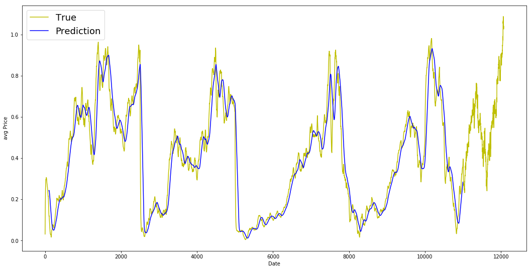

A wide figure is prepared and two time series are drawn on the same axes so their agreement can be inspected visually: the full measured average-price series is plotted across the entire dataset in a yellow line, and the prediction series is plotted in blue beginning at the index where predictions are available. The prediction trace starts later because the forecasting routine only produces values after a certain history window has been seen, so the plotted prediction array aligns with the true series starting at that window boundary rather than from the absolute start.

Axis labels are added to mark the horizontal axis as a date index and the vertical axis as the average price, and a legend identifies which line is the true series versus the prediction. The saved output shows the generated Matplotlib figure (noted as a 1296x648 figure with one axes) and the attached image displays these two overlaid curves across roughly twelve thousand time steps.

Visually, the blue prediction line tracks the yellow true line closely for long stretches, capturing the major rises and falls and the general shape of the series. Where the series makes abrupt spikes or very sharp reversals the prediction sometimes smooths over or slightly lags those extremes, so the blue trace can under- or overshoot briefly; otherwise the peaks and valleys line up well, indicating the predictor reproduces the dominant patterns. The plot therefore provides a quick qualitative assessment: predictions are broadly accurate at the trend level and follow short-term fluctuations reasonably, but occasional sharp deviations remain.

Success — the first prediction from this pipeline looks very good. Contrast this with the earlier notebook, where a different normalization scheme together with a simple averaging baseline was used; the current approach gives a clearly stronger one-step forecast.

Reference: https://www.learndatasci.com/tutorials/python-finance-part-3-moving-average-trading-strategy/

Exponential moving average

We will use an exponential moving average as a simple baseline for one-step-ahead forecasting.

The EMA produces the prediction for the next time step by maintaining a running average that blends the previous EMA value and the current observation. Concretely, at each update the EMA is computed by taking a fraction, called gamma, of the previous EMA and adding the remainder, that is one minus gamma, times the current price. The initial EMA value is set to zero.

Intuitively, gamma controls how quickly the average responds to recent changes: a small value given to the newest observation places more emphasis on the long-run history and yields smoother, more stable predictions. Below we apply this EMA update to generate one-step forecasts and evaluate how well it performs.

window_size = 100
N = train.size
mse_err = []
_avg_predictions_run = []
_avg_x_run = []



running_mean = 0.0 #the mean tat is calculates
_avg_predictions_run.append(running_mean) 

decay = 0.5 # use this to average the running mean again; 

for idx1 in range(1,N): #range from 1 to N-1
     
    running_mean = running_mean*decay + (1.0-decay)*train[idx1-1] #the remaining prob multiplied by the train sets data points
    _avg_predictions_run.append(running_mean)
    mse_err.append((_avg_predictions_run[-1]-train[idx1])**2) #make mse error with the help of train set
    _avg_x_run.append(date) #append the dates into the list

print('MSE error for EMA averaging: %.5f'%(0.5*np.mean(mse_err))) #Calculate MSE

MSE error for EMA averaging: 0.00003

A simple exponential moving average (EMA) is being used as a one-step-ahead forecasting baseline for the training series, and the cell computes the corresponding mean squared error (reported with a 0.5 scaling factor). It begins by preparing a few containers: one to hold squared errors, one to record the EMA predictions as they evolve, and another intended to hold x-values or dates for plotting. The running mean that represents the EMA is initialized to zero and immediately appended to the predictions list so the predictions list has an entry before any updates.

The EMA update uses a decay weight of 0.5, so each new running mean is a 50/50 blend of the previous EMA and the most recent observed training value. Concretely, at each time step t the running mean is multiplied by the decay and then the new observation from t−1 is added in with weight (1 − decay). That running mean is the one-step-ahead prediction for time t, so after updating the running mean the code appends that value to the predictions list and computes the squared error between this prediction and the actual training value at the current time. Those squared errors accumulate in the mse_err list. The date-list append happens every iteration as well, but it simply adds the same date object repeatedly rather than advancing along a time index, so it does not produce a meaningful time axis in its current form.

When the loop finishes, the cell prints half the mean of the accumulated squared errors, which the author labels as the MSE metric. The printed output shows a very small value, 0.00003, because the training series has been scaled to small numeric values and the EMA with a moderate smoothing weight tracks short-term fluctuations reasonably well; both factors make the average squared deviations tiny. Note also that the initial running mean of zero is only present in the predictions list before any update and does not contribute to the first calculated error, because error accumulation starts from the first updated running mean.

Mean squared error shows the exponential moving average substantially outperforms the simple moving average

plt.figure(figsize = (18,9))
plt.plot(range(df.shape[0]),all_avg_data,color='y',label='True Price Stock')
plt.plot(range(0,N),_avg_predictions_run,color='r', label='Prediction')
plt.xlabel('Date')
plt.ylabel('avg Price')
plt.legend(fontsize=18)
plt.show()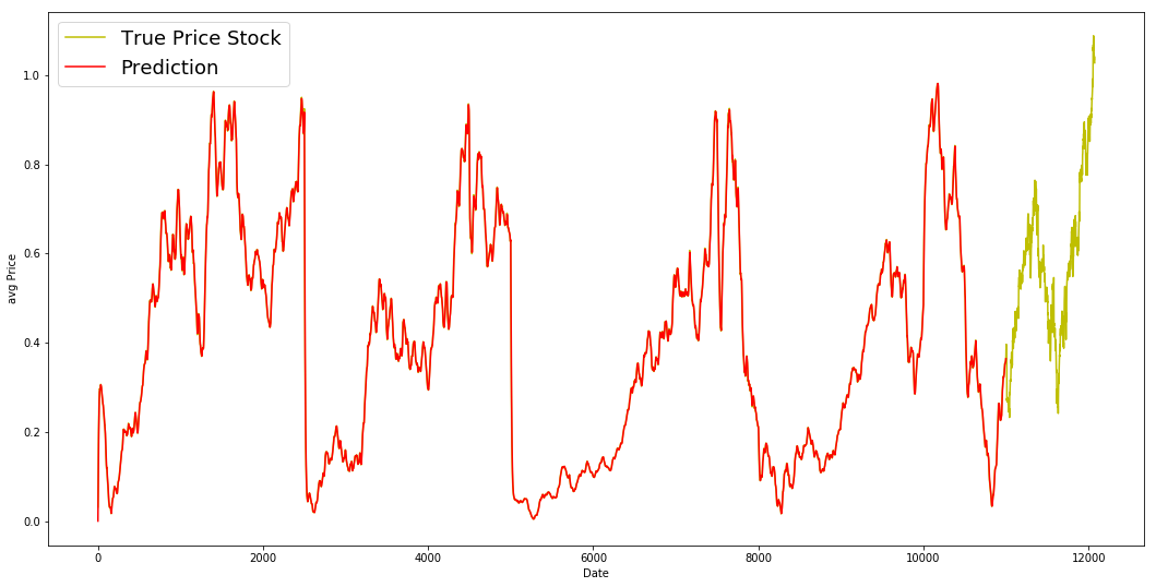

A figure canvas is prepared with a wide rectangular aspect so the time series are easy to inspect along the horizontal axis. Two series are drawn on that canvas: the complete averaged stock price for every day in the dataset is plotted in yellow across the full date range, and a predicted sequence from the model is plotted in red over a shorter prefix of the same timeline. The horizontal axis uses integer positions for days while the vertical axis shows the normalized average price, so values sit roughly between zero and about one on the y scale. Labels for the x and y axes are added and a legend identifies the yellow line as the true, observed average price and the red line as the model prediction, then the figure is rendered to the output.

The textual output line saying the figure size simply reflects that Matplotlib created a 1296 by 648 pixel figure; the attached image is the actual plot. Visually, the red prediction line closely follows the shape of the observed series over the region where predictions were produced, confirming that the model captures many of the ups and downs in that interval. The prediction trace stops short of the far right edge because predictions were generated only for the first N time steps, while the yellow true-price series continues beyond that point for the remainder of the dataset. Where both lines overlap early on the red trace often obscures the yellow one because they are drawn on top of each other. Small abrupt drops or near-zero segments in the red trace correspond to regions where the predicted values differ markedly from the observed series or where the predictor produced low normalized values; these features are a direct consequence of how the model outputs were scaled and where the prediction sequence begins and ends. Overall, the plot provides a straightforward visual comparison: the red curve shows the model’s forecasted path up to N, and the yellow curve shows the ground-truth path across the entire available date range.

The exponential moving average works very well as a baseline for this series. Ideally, a predictive method should reproduce the same overall shape and short-term fluctuations seen in the true data.

Implementation notes. In our code we looped through the time series starting at the second observation and progressing to the end, updating a single running mean by incorporating the per-step averaged value at each iteration. The smoothing weight we applied was one half, so each update blended the new averaged observation with the previous running mean using that coefficient.

See the reference below for a practical discussion of moving-average trading rules.

Reference: https://traderhq.com/moving-average-trading-strategies-do-they-work/

Now we move on to building and training the LSTM model.

Long short-term memory network

In this section we construct and train a recurrent neural network using long short-term memory cells to perform the one-step-ahead forecasting described earlier.

Steps for training and evaluating the LSTM

Prepare the training targets so the model can learn to forecast short-term stock moves.

Apply data augmentation and smoothing procedures to the training series as needed.

Choose model hyperparameters such as batch size, number of unrolled time steps, number of LSTM layers and units, learning rate, and number of epochs.

Construct the model inputs and corresponding target outputs for each unrolled time step.

Specify the LSTM cell configuration and the parameters for the final regression head that maps LSTM outputs to predictions.

Run the LSTM forward pass to obtain the sequence of hidden outputs for each unrolled step.

Convert the LSTM outputs into scalar forecasts using the regression head.

Define the loss function comparing predictions to targets and set up the optimizer (including any gradient clipping or learning-rate schedule).

Train the network by iterating over unrolled batches, updating parameters according to the optimizer.

Produce multi-step predictions on held-out data and plot the predicted sequences against the true series for visual evaluation.

1 : Prepare sequential batches of stock movements for the LSTM

This routine converts the price series into minibatches and matching targets so they can be fed into the LSTM training loop.

What the procedure does

Produce the feature sequences and their corresponding target values.
Build full-length arrays for the sequences and targets, and create an index array drawn from the closing price series.
Break those long sequences into smaller, rolled-out minibatches.
Provide the minibatches as inputs to the LSTM, where each input sequence is paired with its price-based label.

How it works, conceptually

Decide on a minibatch size that will partition the time series into parallel streams.
Divide the sequence into segments according to that batch size and slide through the series to extract shorter sequence chunks.
Implement the rolling extraction inside the unroll method so that multiple time steps are emitted in sequence for each batch.
Treat the extracted sequence chunks as the model inputs and the corresponding future price values as the labels.

class Generator(object):   
    
    def __init__(self,prices,batch_size,num_unroll): #helps to generate data 
        self._prices = prices
        self._prices_length = len(self._prices) - num_unroll
        self._batch_size = batch_size
        self._num_unroll = num_unroll
        self._segments = self._prices_length //self._batch_size
        self._cursor = [offset * self._segments for offset in range(self._batch_size)]

    def next(self):   #which will output a set of num_unrollings batches of input data obtained sequentially, where a batch of data is of size [batch_size, 1]. 
        
        batch_data = np.zeros((self._batch_size),dtype=np.float32)  #Then each batch of input data will have a corresponding output batch of data.
        batch_labels = np.zeros((self._batch_size),dtype=np.float32)
        
        for b in range(self._batch_size):   #create batches 
            if self._cursor[b]+1>=self._prices_length:
                self._cursor[b] = np.random.randint(0,(b+1)*self._segments)
                
            batch_data[b] = self._prices[self._cursor[b]]
            batch_labels[b]= self._prices[self._cursor[b]+np.random.randint(1,5)]
            
            self._cursor[b] = (self._cursor[b]+1)%self._prices_length
            
        return batch_data,batch_labels
    
    def unroll(self):   #roll out the batches generated in form of data and labels 
            
        unroll_data,unroll_labels = [],[]
        init_data, init_label = None,None
        for ui in range(self._num_unroll):
            
            data, labels = self.next()    

            unroll_data.append(data)
            unroll_labels.append(labels)

        return unroll_data, unroll_labels
    
    def reset_indices(self): #get prices length 
        for b in range(self._batch_size):
            self._cursor[b] = np.random.randint(0,min((b+1)*self._segments,self._prices_length-1))
        


dg = Generator(train,5,5)
u_data, u_labels = dg.unroll()

for ui,(dat,lbl) in enumerate(zip(u_data,u_labels)):   
    print('\n\nUnrolled index %d'%ui)
    dat_ind = dat
    lbl_ind = lbl
    print('\tInputs: ',dat )
    print('\n\tOutput:',lbl)



Unrolled index 0
	Inputs:  [0.03143791 0.6904868  0.82829314 0.32585657 0.11600105]

	Output: [0.11098009 0.6848606  0.83294916 0.33355275 0.12106793]


Unrolled index 1
	Inputs:  [0.06067836 0.6890754  0.8325337  0.32857886 0.11785509]

	Output: [0.132895   0.6848606  0.833369   0.33421066 0.12192084]


Unrolled index 2
	Inputs:  [0.08698314 0.68685144 0.8329321  0.33078218 0.11946969]

	Output: [0.132895   0.6848606  0.833141   0.33355275 0.12158521]


Unrolled index 3
	Inputs:  [0.11098009 0.6858036  0.83294916 0.33219692 0.12106793]

	Output: [0.17132245 0.6820074  0.833369   0.33355275 0.12230608]


Unrolled index 4
	Inputs:  [0.132895   0.6848606  0.833369   0.33355275 0.12158521]

	Output: [0.17132245 0.6836884  0.83387965 0.33650374 0.12358698]

A small data-generator class is being implemented to produce sequential training batches for an RNN and then a short demonstration is run to show what those batches look like. The generator takes a one-dimensional price series and parameters that control how many parallel sequences (the batch size) and how many time steps to return in an unrolled chunk. It partitions the available time series into contiguous segments so each batch slot walks through a different portion of the series, and it keeps a cursor for each batch slot that marks the current position inside its segment.

When asked for the next batch, the generator prepares two flat arrays: one for the inputs and one for the labels, each with one entry per parallel sequence. For every batch slot it checks the cursor and, if necessary, reinitializes it randomly within the slot’s segment to avoid wandering past the available data. The input value for a slot is just the price at the cursor position. The associated label is not the immediately next price but a short-future value chosen randomly between one and four steps ahead, so the network is trained to predict a small random lookahead rather than always a fixed one-step target. After producing input and label for a slot the cursor is advanced by one (wrapping inside the allowed range), so subsequent calls naturally move forward along the series.

The unroll method repeatedly calls next the requested number of times and collects the successive batches into two lists: one list of input arrays and one list of label arrays, representing a temporal sequence of batch-sized slices. The reset method (shown but not used in the printout) re-randomizes the cursors within their segments, which is useful to reshuffle where each parallel sequence begins.

The demonstration constructs a generator over the training series with batch size five and unroll length five, asks for a full unrolled chunk, and prints each time slice. The printed “Inputs” lines are the five parallel input values at that time step and the “Output” lines are the corresponding five labels. Because the price data were scaled earlier, these numbers lie between 0 and 1; they look like small decimals for the same reason. Reading across the unrolled indices reveals the sequential behavior: values in the inputs shift gradually from one unrolled index to the next because each cursor advances by one, and some values that appeared as labels in an earlier unroll show up as inputs in a later unroll once the cursor reaches them. The repeated identical numbers in some label slots across different unrolls reflect either that the random lookahead happened to pick the same future index multiple times or that different batch slots happen to reference the same future value due to how segments and randomization were set up.

Overall, the cell prepares a stream of temporally coherent, parallel training examples suitable for truncated backpropagation through time: each call to unroll returns a short time window of batch-sized inputs and corresponding short-horizon targets, and the printed output simply illustrates how those windows move forward through the normalized price series and how the random short lookahead produces slightly offset label values.

2: Hyperparameter tuning

We now adjust model hyperparameters to try and improve the LSTM's performance.

D specifies the input dimensionality. For this notebook it is one, since each time step is represented by a single scalar value and the model predicts a scalar output.
num_unrollings is the number of time steps the network is unrolled during backpropagation through time. This parameter determines how far back in the sequence the model can propagate gradients when updating weights.
batch_size controls how many examples are processed together in a single training update.
num_nodes indicates the number of hidden units inside each LSTM cell. The term layers refers to the architecture’s depth or the list of unit counts for each LSTM layer, i.e., how many layers are stacked and how many units each layer contains.

Refer to the TensorFlow documentation for details on layer construction and related options: https://www.tensorflow.org/api_docs/python/tf/layers/Dense

D = 1 # Dimensionality of the data. Since our data is 1-D this would be 1
num_unrollings = 50 # Number of time steps you look into the future.
batch_size = 500 # Number of samples in a batch
num_nodes = [200,200,150] # Number of hidden nodes in each layer of the deep LSTM stack we're using
n_layers = len(num_nodes) # number of layers
dropout = 0.2 # dropout amount

tf.reset_default_graph() # This is important in case you run this multiple times

Several key hyperparameters for the LSTM experiment are being established: the input dimensionality is set to one, reflecting a single time series value per step; the number of unrolled time steps is set to fifty, which determines how many sequential steps the training graph will backpropagate through at each update; and the batch size is set to five hundred, which controls how many parallel sequences are processed in each training iteration. The network architecture is specified by a list of hidden layer sizes — two hundred units, two hundred units, and one hundred fifty units — and the number of layers is computed from that list. A dropout rate of twenty percent is chosen to regularize the network by randomly omitting a fraction of hidden activations during training.

The TensorFlow default graph is reset so that any previously defined variables, ops, or graphs are cleared before the new model is built; this prevents name collisions and accidental reuse of tensors if the notebook is rerun with different hyperparameters. Because the cell only assigns configuration values and clears the graph, no output is produced or saved. The variables and reset prepare the environment for the subsequent cells that will construct the model, allocate placeholders and state tensors sized according to these choices, and build the training and prediction operations.

Prepare inputs and targets for the model

Partition the training sequence into two arrays: one that will serve as the model inputs and another that will serve as the target outputs. Specify that the input feature dimension is one and that the output feature dimension is also one. Represent the batch size as a one-element tuple. When you construct the tensors to feed the LSTM, provide a shape that describes the batch size followed by the feature dimension; in the notebook this shape is represented using three fields in the code.

train_inputs, train_outputs = [],[]

# You unroll the input over time defining placeholders for each time step
for ui in range(num_unrollings):
    train_inputs.append(tf.placeholder(tf.float32, shape=[batch_size,D],name='train_inputs_%d'%ui))
    train_outputs.append(tf.placeholder(tf.float32, shape=[batch_size,1], name = 'train_outputs_%d'%ui))

Two empty lists are set up to hold placeholders that represent the network inputs and targets at each time step of an unrolled sequence. The loop runs for the configured number of unrollings and, on each iteration, appends one input placeholder and one output placeholder: the input placeholder expects a mini-batch of examples with shape batchsize by D (so the graph will accept batchsize parallel examples, each with D features), and the output placeholder expects the corresponding targets with shape batch_size by 1 (a single scalar target per example). Each placeholder is given a name that includes the time-step index, which helps when inspecting the graph or debugging.

These placeholders do not contain data themselves; they declare the types and shapes of tensors the session must be fed later. During training the code will build a feed dictionary that maps each time-step placeholder to the appropriate slice of the unrolled mini-batch so the model can compute per-step predictions and accumulate loss across the unrolled steps. Using separate placeholders per time step is a typical TF1.x pattern for manual unrolling and for summing losses over time. There is no printed or saved output from this cell — it only prepares the placeholder objects that the subsequent graph construction and training loop will use.

Create one LSTM cell (follow the TensorFlow API reference for exact usage)

lstm_cells = [
    tf.contrib.rnn.LSTMCell(num_units=num_nodes[li],
                            state_is_tuple=True,
                            initializer= tf.contrib.layers.xavier_initializer()
                           )
 for li in range(n_layers)]

drop_lstm_cells = [tf.contrib.rnn.DropoutWrapper(
    lstm, input_keep_prob=1.0,output_keep_prob=1.0-dropout, state_keep_prob=1.0-dropout
) for lstm in lstm_cells]
drop_multi_cell = tf.contrib.rnn.MultiRNNCell(drop_lstm_cells)
multi_cell = tf.contrib.rnn.MultiRNNCell(lstm_cells)

w = tf.get_variable('w',shape=[num_nodes[-1], 1], initializer=tf.contrib.layers.xavier_initializer())
b = tf.get_variable('b',initializer=tf.random_uniform([1],-0.1,0.1))

Here the RNN building blocks and the final projection layer are created so the graph has a stack of LSTM layers and the variables that will turn the last LSTM output into a scalar prediction. The code iterates over the configured number of layers and, for each layer, constructs an LSTM cell object with the layer’s specified number of hidden units. Each cell is told to represent its state as a tuple of (c, h) which keeps the cell state and hidden state separate, and the cell’s internal weights are initialized with a Xavier initializer to help keep gradients and activations well-scaled at the start of training.

After the raw LSTM cells are made, dropout wrappers are applied to them. The wrappers are configured so that the cell inputs are not dropped but the cell outputs and the recurrent state can be dropped according to the dropout hyperparameter; concretely, outputkeepprob and statekeepprob are set to one minus the dropout rate. Wrapping each layer this way yields a dropout-enabled stack which is then combined into a single multi-layer recurrent unit using a MultiRNNCell. A second MultiRNNCell is also constructed from the original, non-dropped LSTM cells; having both versions is a common pattern so the training-time cell with dropout and the evaluation/inference-time cell without dropout are both available in the graph.

The final affine transformation that maps from the top LSTM layer’s hidden dimension down to a single prediction is prepared by creating two variables: a weight matrix whose number of rows matches the last layer’s hidden size and whose single column produces the scalar output, and a bias scalar initialized uniformly in a small range. The weight uses a Xavier initializer to promote stable learning, while the bias is given a small random start. Executing these operations does not print anything; it instantiates the cell objects and registers the variables in the TensorFlow graph so later operations (unrolling the network, computing outputs and losses, or restoring states) can use them.

Next steps

The remaining work is to prepare the inputs for the network, implement how the model measures its error, wire that error into an optimization step, and then run the training loop for the LSTM. In practice that means: transform and shape the sequence inputs appropriately, compute the training loss, connect an optimizer to minimize that loss, and execute the training iterations.

Relevant TensorFlow documentation pages:

Dynamic RNN: https://www.tensorflow.org/apidocs/python/tf/nn/dynamicrnn — reference for running recurrent cells over time series inputs.
Optimizer base class and implementations: https://www.tensorflow.org/api_docs/python/tf/train/Optimizer — details on optimization algorithms and applying gradients.
Reshape operation: https://www.tensorflow.org/api_docs/python/tf/reshape — how to change tensor shapes when preparing batched sequences or model outputs.
Control dependencies: https://www.tensorflow.org/apidocs/python/tf/controldependencies — ensuring correct execution order for state updates and grouped operations.

# Create cell state and hidden state variables to maintain the state of the LSTM
a1, b1 = [],[]
initial_state = []
for li in range(n_layers):
  a1.append(tf.Variable(tf.zeros([batch_size, num_nodes[li]]), trainable=False))
  b1.append(tf.Variable(tf.zeros([batch_size, num_nodes[li]]), trainable=False))
  initial_state.append(tf.contrib.rnn.LSTMStateTuple(a1[li], b1[li]))

# Do several tensor transofmations, because the function dynamic_rnn requires the output to be of
# a specific format. 
all_inputs = tf.concat([tf.expand_dims(t,0) for t in train_inputs],axis=0)

# all_outputs is [seq_length, batch_size, num_nodes]
all_lstm_outputs, state = tf.nn.dynamic_rnn(
    drop_multi_cell, all_inputs, initial_state=tuple(initial_state),
    time_major = True, dtype=tf.float32)

all_lstm_outputs = tf.reshape(all_lstm_outputs, [batch_size*num_unrollings,num_nodes[-1]])

all_outputs = tf.nn.xw_plus_b(all_lstm_outputs,w,b)

split_outputs = tf.split(all_outputs,num_unrollings,axis=0)

Several per-layer tensors are allocated to hold the LSTM's internal state across batches so the network can carry memory from one minibatch to the next during truncated backpropagation through time. For each layer, a pair of zero-initialized variables is created to represent the LSTM's cell state and hidden state; these variables are marked non-trainable so they are not adjusted by the optimizer but can be updated explicitly between training steps. Those per-layer pairs are wrapped into the framework's LSTM state tuple format and collected into an initial_state structure that will be supplied to the recurrent network when it runs.

The next step prepares the sequence input in the specific layout expected by the dynamic RNN implementation. The collection of inputs that represent each unrolled time step is converted into a single three-dimensional tensor with time as the first dimension, batch as the second, and features as the third (a time-major layout). That transformation is necessary because the dynamic RNN routine is designed to process a time-major tensor so it can iterate efficiently over timesteps.

Calling the dynamic RNN executes the stacked, dropout-wrapped LSTM across the full unrolled sequence starting from the provided initial state. The call returns two things: the sequence of hidden outputs at every timestep for every batch element, and the final LSTM state after running through the whole unrolled window. The output tensor coming back has the shape [sequencelength, batchsize, numberofunitsinlast_layer], reflecting one vector per timestep and per batch entry.

Because the following prediction layer expects a two-dimensional input where each row is a single feature vector to be linearly projected to a scalar prediction, the time-major 3D output is reshaped so that the time and batch axes are merged into one first axis, producing a two-dimensional tensor with rows equal to batchsize times numberof_unrollings and columns equal to the size of the final LSTM layer. A linear affine transformation (matrix multiply plus bias) is applied to every row to produce raw output values for every timestep and batch element.

Finally, those flattened outputs are split back into a list of tensors, one per unrolled timestep, so they line up with the corresponding target tensors used to compute the loss. There is no printed or saved result from running this cell; instead it constructs and wires up the variables and tensors needed for training and evaluation: the persistent LSTM states, the input-to-RNN formatting, the recurrent computation itself, the projection to predictions, and the organization of outputs into per-timestep slices that downstream loss and optimizer operations will consume.

# When calculating the loss you need to be careful about the exact form, because you calculate
# loss of all the unrolled steps at the same time
# Therefore, take the mean error or each batch and get the sum of that over all the unrolled steps
print('Loss for the input train while converting prices into movements')
loss = 0.0
with tf.control_dependencies([tf.assign(a1[li], state[li][0]) for li in range(n_layers)]+
                             [tf.assign(b1[li], state[li][1]) for li in range(n_layers)]):
  for ui in range(num_unrollings):
    loss += tf.reduce_mean(0.5*(split_outputs[ui]-train_outputs[ui])**2)

print('Learning rate decay operations')
global_step = tf.Variable(0, trainable=False)
inc_gstep = tf.assign(global_step,global_step + 1)
tf_learning_rate = tf.placeholder(shape=None,dtype=tf.float32)
tf_min_learning_rate = tf.placeholder(shape=None,dtype=tf.float32)

learning_rate = tf.maximum(
    tf.train.exponential_decay(tf_learning_rate, global_step, decay_steps=1, decay_rate=0.5, staircase=True),
    tf_min_learning_rate)

# Optimizer.
print('TF Optimization operations')
optimizer = tf.train.AdamOptimizer(learning_rate)
gradients, v = zip(*optimizer.compute_gradients(loss))
gradients, _ =  tf.clip_by_global_norm(gradients, 5.0)
optimizer = optimizer.apply_gradients(
    zip(gradients, v))

Loss for the input train while converting prices into movements
Learning rate decay operations
TF Optimization operations

The cell sets up how the model will measure error over an unrolled sequence and how it will be optimized, including learning-rate scheduling and gradient clipping. It first declares a loss tensor that accumulates the mean squared error across the unrolled time steps: for each time step the mean over the batch of 0.5 times the squared difference between the model's prediction and the target is computed, and those per-step means are added together. Wrapping the loss construction in a control-dependency block forces the graph to assign the current LSTM state variables from the provided state tensors for every layer before any of the loss computations run, ensuring that the loss is always evaluated with the intended hidden and cell states in place rather than with stale state values.

Next, the cell prepares learning-rate control logic by creating a non-trainable global step variable and an increment operation for it, plus two placeholders that let the training loop feed a starting learning rate and a minimum allowable learning rate at run time. The effective learning rate used by the optimizer is defined as an exponential decay of the fed initial rate (with a halving behavior due to the chosen decay settings) but floored at the provided minimum, so the training loop can both decay the rate automatically and guarantee it never falls below a safety threshold.

For optimization, an adaptive Adam optimizer is constructed using that computed learning rate. Gradients of the previously built loss with respect to trainable variables are computed, then globally clipped by norm to 5.0 to prevent exploding gradients that are common in recurrent networks. After clipping, those gradients are applied back to their variables to produce the optimizer operation that will be executed during training.

The three printed lines that appear in the saved output correspond to the three print statements interleaved with these graph-construction steps; they are emitted immediately during graph building and indicate the phases that were just set up ("Loss for the input...", "Learning rate decay operations", and "TF Optimization operations"). Because this cell only builds TensorFlow graph nodes and not a session execution, the printed lines are the only runtime output here; the loss and optimizer are now defined as tensors and ops that will be evaluated and executed later inside a training session.

Generate example predictions from the trained network

To produce single-step outputs and updated recurrent states from the LSTM, consult the TensorFlow documentation for the recurrent helper that runs the RNN and returns both the sequence outputs and the final state: https://www.tensorflow.org/apidocs/python/tf/nn/dynamicrnn. Use that behavior to obtain the network output tensor and the new cell and hidden states you will carry forward for iterative prediction.

After obtaining RNN outputs, apply a linear projection to map the hidden activations to prediction values. The small utility that performs a matrix multiply plus a bias term is documented here: https://www.tensorflow.org/apidocs/python/tf/nn/xwplus_b. Use it (or an equivalent dense layer) to convert each time-step output into a scalar forecast.

For implementation examples and additional context on assembling these pieces into a time-series predictor, see this reference repository which I consulted during development: https://github.com/jaungiers/LSTM-Neural-Network-for-Time-Series-Prediction/blob/master/core/model.py

 print('Defining prediction related TF functions')

sample_inputs = tf.placeholder(tf.float32, shape=[1,D])

# Maintaining LSTM state for prediction stage
sample_c, sample_h, initial_sample_state = [],[],[]
for li in range(n_layers):
  sample_c.append(tf.Variable(tf.zeros([1, num_nodes[li]]), trainable=False))
  sample_h.append(tf.Variable(tf.zeros([1, num_nodes[li]]), trainable=False))
  initial_sample_state.append(tf.contrib.rnn.LSTMStateTuple(sample_c[li],sample_h[li]))

reset_sample_states = tf.group(*[tf.assign(sample_c[li],tf.zeros([1, num_nodes[li]])) for li in range(n_layers)],
                               *[tf.assign(sample_h[li],tf.zeros([1, num_nodes[li]])) for li in range(n_layers)])

sample_outputs, sample_state = tf.nn.dynamic_rnn(multi_cell, tf.expand_dims(sample_inputs,0),
                                   initial_state=tuple(initial_sample_state),
                                   time_major = True,
                                   dtype=tf.float32)

with tf.control_dependencies([tf.assign(sample_c[li],sample_state[li][0]) for li in range(n_layers)]+
                              [tf.assign(sample_h[li],sample_state[li][1]) for li in range(n_layers)]):  
  sample_prediction = tf.nn.xw_plus_b(tf.reshape(sample_outputs,[1,-1]), w, b)

print('\tAll done')

Defining prediction related TF functions
	All done

The cell sets up the TensorFlow pieces used to run the trained LSTM one step at a time during inference and to carry its internal recurrent state forward from one prediction to the next. It begins by declaring a single-sample input placeholder with the shape of one example (one batch row with D features), because inference will feed the network one time step at a time rather than whole batches of training data.

To hold the LSTM’s internal state between calls, the code creates per-layer state variables for the cell state and hidden state. Each layer gets two non-trainable variables initialized to zeros: one for the c vector and one for the h vector. Those pairs are wrapped into LSTM state structures so they can be supplied to the RNN as an initial state. Marking these as non-trainable makes it clear they are only used for carrying state during prediction and are not optimized by the training process.

A grouped reset operation is also prepared that assigns zeros into every layer’s state variables. That grouped op provides a convenient single call to clear the LSTM state whenever inference should start from a fresh sequence.

For producing a single-step prediction the LSTM is run with a dynamic RNN call. The single-sample placeholder is given an extra leading dimension so the RNN receives a tensor with explicit time and batch axes; with time-major ordering this corresponds to one time step and one batch element. The RNN invocation uses the per-layer variables created earlier as its initial state, and it returns both the output at that time step and the new state for every layer.

Immediately after the RNN run, the newly produced per-layer states are written back into the non-trainable state variables so that the next call will pick up where this one left off. This update is wired into the graph via a control dependency, ensuring the state assignments complete before the final prediction value is computed. The prediction itself is produced by flattening the RNN’s time-step output and applying the trained linear layer (the saved weight and bias) to produce the scalar forecast for the next value.

Because the state variables are continually updated by these assignments, repeated execution of the prediction operation implements an autoregressive loop: give the network one input, get a prediction, feed that prediction back as the input on the next call, and the LSTM will use its persisted c/h variables to maintain temporal context across steps. When a new independent prediction sequence is desired, running the grouped reset operation clears all states to zeros first.

The two printed lines shown in the saved output simply confirm that these prediction-related operations were defined: the first line appears before building the graph nodes and the second prints after all the state variables, reset op, dynamic RNN call, state-updates, and prediction node have been created, indicating successful construction of the inference machinery.

Define and train the model, then run validation and evaluation and produce forecasts. The implementation follows examples and patterns from the TensorFlow documentation.

epochs = 50
valid_summary = 1 # Interval you make test predictions

n_predict_once = 50 # Number of steps you continously predict for

train_seq_length = train.size # Full length of the training data

train_mse_ot = [] # Accumulate Train losses
test_mse_ot = [] # Accumulate Test loss
predictions_over_time = [] # Accumulate predictions

session = tf.InteractiveSession()

tf.global_variables_initializer().run()

# Used for decaying learning rate
loss_nondecrease_count = 0
loss_nondecrease_threshold = 2 # If the test error hasn't increased in this many steps, decrease learning rate

print('Initialized')
average_loss = 0

# Define data generator
data_gen = Generator(train,batch_size,num_unrollings) 

x_axis_seq = []

# Points you start our test predictions from
test_points_seq = np.arange(11000,12000,50).tolist() 

for ep in range(epochs):       
    
    #Training
    for step in range(train_seq_length//batch_size):
        
        u_data, u_labels = data_gen.unroll()

        feed_dict = {}
        for ui,(dat,lbl) in enumerate(zip(u_data,u_labels)):            
            feed_dict[train_inputs[ui]] = dat.reshape(-1,1)
            feed_dict[train_outputs[ui]] = lbl.reshape(-1,1)
        
        feed_dict.update({tf_learning_rate: 0.0001, tf_min_learning_rate:0.000001})

        _, l = session.run([optimizer, loss], feed_dict=feed_dict)

        average_loss += l
    
    #Validation
    if (ep+1) % valid_summary == 0:

      average_loss = average_loss/(valid_summary*(train_seq_length//batch_size))
      
      # The average loss
      if (ep+1)%valid_summary==0:
        print('Average loss at step %d: %f' % (ep+1, average_loss))
      
      train_mse_ot.append(average_loss)
            
      average_loss = 0 # reset loss
      
      predictions_seq = []
      
      mse_test_loss_seq = []
      
      #Updating State and Making Predicitons
      for w_i in test_points_seq:
        mse_test_loss = 0.0
        our_predictions = []
        
        if (ep+1)-valid_summary==0:
          # Only calculate x_axis values in the first validation epoch
          x_axis=[]
        
        # Feed in the recent past behavior of stock prices
        # to make predictions from that point onwards
        for tr_i in range(w_i-num_unrollings+1,w_i-1):
          current_price = all_avg_data[tr_i]
          feed_dict[sample_inputs] = np.array(current_price).reshape(1,1)    
          _ = session.run(sample_prediction,feed_dict=feed_dict)
        
        feed_dict = {}
        
        current_price = all_avg_data[w_i-1]
        
        feed_dict[sample_inputs] = np.array(current_price).reshape(1,1)
        
        # Make predictions for this many steps
        # Each prediction uses previous prediciton as it's current input
        for pred_i in range(n_predict_once):

          pred = session.run(sample_prediction,feed_dict=feed_dict)
        
          our_predictions.append(np.asscalar(pred))
        
          feed_dict[sample_inputs] = np.asarray(pred).reshape(-1,1)

          if (ep+1)-valid_summary==0:
            # Only calculate x_axis values in the first validation epoch
            x_axis.append(w_i+pred_i)

          mse_test_loss += 0.5*(pred-all_avg_data[w_i+pred_i])**2
        
        session.run(reset_sample_states)
        
        predictions_seq.append(np.array(our_predictions))
        
        mse_test_loss /= n_predict_once
        mse_test_loss_seq.append(mse_test_loss)
        
        if (ep+1)-valid_summary==0:
          x_axis_seq.append(x_axis)
        
      current_test_mse = np.mean(mse_test_loss_seq)
      
      # Learning rate decay logic
      if len(test_mse_ot)>0 and current_test_mse > min(test_mse_ot):
          loss_nondecrease_count += 1
      else:
          loss_nondecrease_count = 0
      
      if loss_nondecrease_count > loss_nondecrease_threshold :
            session.run(inc_gstep)
            loss_nondecrease_count = 0
            print('\tDecreasing learning rate by 0.5')
      
      test_mse_ot.append(current_test_mse)
      print('\tTest MSE: %.5f'%np.mean(mse_test_loss_seq))
      predictions_over_time.append(predictions_seq)
      print('\tFinished Predictions')

/usr/local/lib/python3.6/dist-packages/tensorflow/python/client/session.py:1735: UserWarning: An interactive session is already active. This can cause out-of-memory errors in some cases. You must explicitly call `InteractiveSession.close()` to release resources held by the other session(s).
  warnings.warn('An interactive session is already active. This can '

Initialized
Average loss at step 1: 1.606525
	Test MSE: 0.01014
	Finished Predictions
Average loss at step 2: 0.176963
	Test MSE: 0.00842
	Finished Predictions
Average loss at step 3: 0.080844
	Test MSE: 0.00311
	Finished Predictions
Average loss at step 4: 0.066810
	Test MSE: 0.00270
	Finished Predictions
Average loss at step 5: 0.055696
	Test MSE: 0.00270
	Finished Predictions
Average loss at step 6: 0.052513
	Test MSE: 0.00345
	Finished Predictions
Average loss at step 7: 0.052445
	Test MSE: 0.00243
	Finished Predictions
Average loss at step 8: 0.046246
	Test MSE: 0.00242
	Finished Predictions
Average loss at step 9: 0.050750
	Test MSE: 0.00241
	Finished Predictions
Average loss at step 10: 0.043253
	Test MSE: 0.00240
	Finished Predictions
Average loss at step 11: 0.040725
	Test MSE: 0.00273
	Finished Predictions
Average loss at step 12: 0.039212
	Test MSE: 0.00238
	Finished Predictions
Average loss at step 13: 0.036308
	Test MSE: 0.00239
	Finished Predictions
Average loss at step 14: 0.035945
	Test MSE: 0.00315
	Finished Predictions
Average loss at step 15: 0.031898
	Decreasing learning rate by 0.5
	Test MSE: 0.00240
	Finished Predictions
Average loss at step 16: 0.034355
	Test MSE: 0.00250
	Finished Predictions
Average loss at step 17: 0.034596
	Test MSE: 0.00260
	Finished Predictions
Average loss at step 18: 0.033832
	Decreasing learning rate by 0.5
	Test MSE: 0.00242
	Finished Predictions
Average loss at step 19: 0.035760
	Test MSE: 0.00275
	Finished Predictions
Average loss at step 20: 0.033869
	Test MSE: 0.00264
	Finished Predictions
Average loss at step 21: 0.034513
	Decreasing learning rate by 0.5
	Test MSE: 0.00240
	Finished Predictions
Average loss at step 22: 0.035446
	Test MSE: 0.00243
	Finished Predictions
Average loss at step 23: 0.031067
	Test MSE: 0.00241
	Finished Predictions
Average loss at step 24: 0.029816
	Decreasing learning rate by 0.5
	Test MSE: 0.00248
	Finished Predictions
Average loss at step 25: 0.032785
	Test MSE: 0.00245
	Finished Predictions
Average loss at step 26: 0.030762
	Test MSE: 0.00249
	Finished Predictions
Average loss at step 27: 0.033554
	Decreasing learning rate by 0.5
	Test MSE: 0.00245
	Finished Predictions
Average loss at step 28: 0.032914
	Test MSE: 0.00244
	Finished Predictions
Average loss at step 29: 0.032163
	Test MSE: 0.00242
	Finished Predictions
Average loss at step 30: 0.033407
	Decreasing learning rate by 0.5
	Test MSE: 0.00243
	Finished Predictions
Average loss at step 31: 0.032234
	Test MSE: 0.00246
	Finished Predictions
Average loss at step 32: 0.032712
	Test MSE: 0.00247
	Finished Predictions
Average loss at step 33: 0.032348
	Decreasing learning rate by 0.5
	Test MSE: 0.00245
	Finished Predictions
Average loss at step 34: 0.032165
	Test MSE: 0.00248
	Finished Predictions
Average loss at step 35: 0.031905
	Test MSE: 0.00246
	Finished Predictions
Average loss at step 36: 0.032236
	Decreasing learning rate by 0.5
	Test MSE: 0.00245
	Finished Predictions
Average loss at step 37: 0.031640
	Test MSE: 0.00244
	Finished Predictions
Average loss at step 38: 0.033074
	Test MSE: 0.00243
	Finished Predictions
Average loss at step 39: 0.033712
	Decreasing learning rate by 0.5
	Test MSE: 0.00244
	Finished Predictions
Average loss at step 40: 0.032567
	Test MSE: 0.00248
	Finished Predictions
Average loss at step 41: 0.032738
	Test MSE: 0.00244
	Finished Predictions
Average loss at step 42: 0.033136
	Decreasing learning rate by 0.5
	Test MSE: 0.00246
	Finished Predictions
Average loss at step 43: 0.030617
	Test MSE: 0.00245
	Finished Predictions
Average loss at step 44: 0.032362
	Test MSE: 0.00244
	Finished Predictions
Average loss at step 45: 0.032597
	Decreasing learning rate by 0.5
	Test MSE: 0.00246
	Finished Predictions
Average loss at step 46: 0.032263
	Test MSE: 0.00246
	Finished Predictions
Average loss at step 47: 0.031943
	Test MSE: 0.00246
	Finished Predictions
Average loss at step 48: 0.032538
	Decreasing learning rate by 0.5
	Test MSE: 0.00244
	Finished Predictions
Average loss at step 49: 0.031622
	Test MSE: 0.00243
	Finished Predictions
Average loss at step 50: 0.034074
	Test MSE: 0.00245
	Finished Predictions

Setup for the training and validation run is performed by defining how many epochs to run, how often to produce validation predictions, how many autoregressive prediction steps to make during each validation, and by allocating containers to collect training losses, test losses and predicted sequences over time. A TensorFlow interactive session is started and all model variables are initialized so the optimizer, RNN weights and any state-holding tensors are ready to use. A small warning appears in the saved output about an already-active interactive session; that simply signals that another session object was not closed previously and can be ignored here, although in long runs it can cause extra memory use unless the older session is closed.

A data generator instance is created to supply unrolled batches for training and a list of test starting indices is prepared; these starting points mark where in the full price series the script will seed the RNN and then produce multi-step predictions. The outer loop iterates over epochs. Inside each epoch the code iterates over the number of training steps determined by the training sequence length divided by the batch size. For every training step the generator produces a sequence of unrolled input batches and the corresponding target values; these are placed into the feed dictionary by mapping each unrolled time-step placeholder to its batch of inputs and targets. A small fixed learning-rate schedule value is put in the feed dictionary and then the session runs the optimizer and returns the batch loss. Losses from all steps of the epoch are accumulated into average_loss so they can be reported as an epoch-level average.

Validation occurs at the interval specified by validsummary, which in this run is every epoch. The accumulated averageloss is normalized by the number of training steps and printed; that value is also stored for plotting or inspection as the per-epoch training loss. Validation then proceeds by iterating over every test starting index. For each start point the recent numunrollings−1 real prices immediately preceding the start are fed one at a time into the sample prediction graph. Running the single-step sample prediction repeatedly with those real prices warms up the LSTM sample state so that its hidden and cell states reflect the recent history before actual forecasting begins. After warming up, the code enters an autoregressive loop that requests npredictonce successive single-step predictions. Each predicted scalar is appended to the sequence of predictions and immediately fed back as the next input so the network effectively rolls forward using its own outputs. A running test loss for that starting point accumulates 0.5*(prediction − truevalue)^2 for each prediction and is averaged across the prediction horizon to give a single test MSE for that start. After the block of predictions finishes the sample states are reset to avoid leakage into the next starting point, and the predicted sequence plus its averaged test MSE are recorded.

Once predictions have been produced for every chosen test start, the code computes the mean test MSE across all starts to get the epoch’s validation metric. A simple learning-rate control mechanism compares this epoch’s test MSE against past values: if the metric has not improved beyond prior bests for more than a small threshold of validation rounds, a step is taken to increment a global step variable that triggers learning-rate decay in the optimizer, and a message is printed to indicate the decay. The epoch’s validation MSE and the collection of prediction sequences are appended to historical lists so the evolution of predictions and test error can be analyzed later.

The saved standard output records these printed quantities for each epoch. After initialization the first epoch shows a very large average training loss (about 1.6065) and a relatively larger test error compared with later epochs; as training proceeds the average training loss falls rapidly in early epochs and then more slowly, stabilizing in the 0.03 range. The test MSE, printed after each epoch, quickly drops into the low 0.002–0.003 range and then fluctuates there. Lines that read "Decreasing learning rate by 0.5" appear intermittently and correspond to the decay logic triggering when the validation MSE did not improve for the configured number of checks. Each epoch ends with the message "Finished Predictions", indicating that the multi-start autoregressive validation sweep completed and the predicted sequences for that epoch were stored.

Taken together, the printed sequence of average losses and test MSEs shows the typical behavior of a trained recurrent network: a large initial training loss followed by rapid early improvement, then a slower convergence phase with small fluctuations in validation error. The separate training and validation metrics come from slightly different computations — training loss is accumulated batch-by-batch during gradient updates, while test MSE is the average of autoregressive multi-step prediction errors across many start points — which is why their numeric magnitudes and dynamics do not match exactly but both reflect the model’s overall improvement.

Visualize TensorFlow model forecasts

This cell draws the LSTM-generated predictions alongside the true series for the test interval. The plotting approach is adapted from TensorFlow's time series tutorial: https://www.tensorflow.org/beta/tutorials/text/time_series

best_prediction_epoch = 49 # replace this with the epoch that you got the best results when running the plotting code

plt.figure(figsize = (18,18))
plt.subplot(2,1,1)
plt.plot(range(df.shape[0]),all_avg_data,color='y',label='data')

# Plotting how the predictions change over time
# Plot older predictions with low alpha and newer predictions with high alpha
start_alpha = 0.25
alpha  = np.arange(start_alpha,1.1,(1.0-start_alpha)/len(predictions_over_time[::3]))
for p_i,p in enumerate(predictions_over_time[::3]):
    for xval,yval in zip(x_axis_seq,p):
        plt.plot(xval,yval,color='b',alpha=alpha[p_i],label='stock price movement change')

plt.title('Different test prediction models',fontsize=18)
plt.xlabel('Days',fontsize=18)
plt.ylabel('avg Price',fontsize=18)
plt.xlim(11000,12500)

plt.subplot(2,1,2)

# Predicting the best test prediction you got
plt.plot(range(df.shape[0]),all_avg_data,color='g',label='predictions')
for xval,yval in zip(x_axis_seq,predictions_over_time[best_prediction_epoch]):
    plt.plot(xval,yval,color='b',label='change in price movement')
    
plt.title('Top Predictions wrt time',fontsize=18)
plt.xlabel('Days',fontsize=18)
plt.ylabel('avg Price',fontsize=18)
plt.xlim(11000,12500)
plt.show()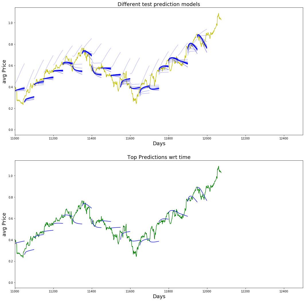

It begins by choosing a single epoch index (49) to highlight as the "best" prediction run and then builds a large two-row figure that overlays the true averaged price series with the model's short-term forecasts. The top panel draws the entire averaged-price time series across all days as a continuous yellow line so you can see the real historical behavior, and then it paints many short multi-day forecast segments in blue at the test locations. Those blue segments are plotted for a subset of saved prediction snapshots (every third saved epoch) and their transparency is ramped from faint to bold: older predictions are drawn with low alpha so they appear pale, while newer ones are drawn with higher alpha and stand out. The plotted forecast segments are positioned using the same day indices as the true series, and the horizontal axis is cropped to the test region (roughly days 11000 to 12500) so the local prediction behavior is easy to inspect.

The bottom panel repeats the true averaged-price series (this time in green) and overlays only the forecasts from the single epoch chosen as best (epoch 49) in solid blue. This gives a focused view of how that single selected model run tracks the actual series: the blue segments tend to follow short-term trends and capture the general direction of movement, but they are smoother and sometimes lag or under/overshoot sharp local peaks and troughs. Looking at the top panel together with the bottom panel makes it clear how the model's predictions evolved across training: many of the earlier, fainter forecasts show larger dispersion and less adherence to the true curve, while later, bolder forecasts cluster closer to the real data and display more consistent short-horizon trend-following.

The notebook's saved output is the two-panel figure described above; the textual display shows the usual matplotlib figure metadata and the image itself is attached. Viewing that image confirms the visual patterns explained here: multiple faint-to-bold blue prediction arcs over the yellow truth in the top plot, and the green truth with the single highlighted blue prediction sequence in the bottom plot, both focused on the test-day interval printed on the x-axis and measured against the averaged price on the y-axis.

Conclusions and interpretation of the plot

The model is estimating price movement rather than forecasting the raw price level. The plotted signals represent normalized movement indicators, not dollar values.
The blue tick marks highlight points where the model indicates a change in movement, in other words locations where momentum shifts are detected.
Those markers are derived from the outputs produced by the sequence-unrolling data generator: the generator’s successive predictions are compared to reveal transitions in the predicted movement signal.
The vertical scale on the plot runs from zero to one, and every predicted movement value lies inside that interval. Values near eighty percent and above, approaching one, correspond to strong model signals.
Across longer periods, the LSTM tends to identify directional movement patterns more effectively than it reconstructs exact price trajectories. In practice this means the network is better at signaling when the market is moving up or down than at returning precise price levels.

Rebuild the sequence batch generator

class Generator(object):   
    
    def __init__(self,prices,batch_size,num_unroll): #helps to generate data 
        self._prices = prices
        self._prices_length = len(self._prices) - num_unroll
        self._batch_size = batch_size
        self._num_unroll = num_unroll
        self._segments = self._prices_length //self._batch_size
        self._cursor = [offset * self._segments for offset in range(self._batch_size)]

    def next(self):   #which will output a set of num_unrollings batches of input data obtained sequentially, where a batch of data is of size [batch_size, 1]. 
        
        batch_data = np.zeros((self._batch_size),dtype=np.float32)  #Then each batch of input data will have a corresponding output batch of data.
        batch_labels = np.zeros((self._batch_size),dtype=np.float32)
        
        for b in range(self._batch_size):   #create batches 
            if self._cursor[b]+1>=self._prices_length:
                self._cursor[b] = np.random.randint(0,(b+1)*self._segments)
                
            batch_data[b] = self._prices[self._cursor[b]]
            batch_labels[b]= self._prices[self._cursor[b]+np.random.randint(1,5)]
            
            self._cursor[b] = (self._cursor[b]+1)%self._prices_length
            
        return batch_data,batch_labels
    
    def unroll(self):   #roll out the batches generated in form of data and labels 
            
        unroll_data,unroll_labels = [],[]
        init_data, init_label = None,None
        for ui in range(self._num_unroll):
            
            data, labels = self.next()    

            unroll_data.append(data)
            unroll_labels.append(labels)

        return unroll_data, unroll_labels
    
    def reset_indices(self): #get prices length 
        for b in range(self._batch_size):
            self._cursor[b] = np.random.randint(0,min((b+1)*self._segments,self._prices_length-1))
        


dg = Generator(train,5,5)
u_data, u_labels = dg.unroll()

for ui,(dat,lbl) in enumerate(zip(u_data,u_labels)):   
    print('\n\nUnrolled index %d'%ui)
    dat_ind = dat
    lbl_ind = lbl
    print('\tInputs: ',dat )
    print('\n\tOutput:',lbl)



Unrolled index 0
	Inputs:  [0.31437907 0.68251073 0.8827639  0.34908384 0.12648556]

	Output: [0.32384238 0.67637324 0.8365174  0.34575522 0.13545202]


Unrolled index 1
	Inputs:  [0.32384238 0.67637324 0.87069887 0.35307965 0.1345414 ]

	Output: [0.33012915 0.67637324 0.8365174  0.34492955 0.1340011 ]


Unrolled index 2
	Inputs:  [0.32372627 0.6668353  0.8365174  0.35061213 0.1340011 ]

	Output: [0.33012915 0.6731387  0.831089   0.34013176 0.1262407 ]


Unrolled index 3
	Inputs:  [0.32695258 0.67637324 0.83310276 0.34492955 0.13545202]

	Output: [0.33012915 0.6731387  0.83714783 0.35714167 0.12494157]


Unrolled index 4
	Inputs:  [0.33012915 0.67637324 0.83714783 0.34575522 0.1262407 ]

	Output: [0.3396588  0.6731387  0.8405274  0.35714167 0.12577325]

The cell builds a small data generator that emits sequential mini-batches of prices and corresponding short-horizon targets, then demonstrates its behavior by producing five unrolled steps of five-element batches. The generator is initialized with a price sequence, a batch size and a number of unrolling steps; it divides the usable portion of the price series into contiguous segments equal to the batch size and places an independent cursor at the start of each segment so each batch element walks through a different region of the series in parallel.

When the generator is asked for the next batch, it allocates two arrays of length batchsize for inputs and labels. For each batch index it checks whether the cursor is near the end of the usable range and, if so, reinitializes that cursor randomly within its segment to avoid running past the end. It writes the input as the price at the cursor position and writes the label as a price a small random number of steps ahead (the random lookahead is uniformly chosen between 1 and 4). After sampling, the cursor advances by one position (wrapping around the usable length). Returning a batch therefore gives you one time slice of size batchsize where each element is a current price and a randomly chosen short-term future price for that same element’s cursor.

Unrolling is implemented by calling the next-batch routine repeatedly num_unroll times and collecting those per-step batches into two lists: a list of input arrays and a list of label arrays. The reset routine (not used in the printed demo) can re-randomize the cursors at segment-appropriate starting locations.

The demonstration creates a generator with batch_size 5 and unroll length 5, obtains the unrolled lists and prints each time step. The saved output shows five blocks labeled Unrolled index 0 through 4. Each block displays an Inputs line with five normalized price values and an Output line with the five corresponding labels chosen by the random lookahead. You can see continuity across successive unrolled indices because each cursor advances by one each step: many numbers reappear shifted between rows, and occasionally a label in one row matches an input in the next row when the chosen lookahead was one. For example, the value 0.32384238 appears as a label in the first unrolled step and then as an input in the second step, illustrating that a one-step lookahead was selected for that cursor. The occasional repeated values and the small differences between inputs and labels reflect the underlying price sequence and the random short-horizon targets; together these behaviors confirm that the generator produces parallel, sequential mini-batches suitable for training an RNN with truncated backpropagation through time.

Start a new training run using altered hyperparameter settings and an updated epoch budget

Adjust the hyperparameters

Edit the model and training configuration before running the next cells. Typical values you might change include the number of unrolled time steps, the batch size, the sizes of each LSTM layer, dropout rate, number of training epochs, and the optimizer learning rate or its decay schedule. After making changes, rebuild the TensorFlow graph and re-run the training cells so the new settings are applied.

D = 1 # Dimensionality of the data. Since our data is 1-D this would be 1
num_unrollings = 75
batch_size = 300
num_nodes = [250,250,175] # Number of hidden nodes in each layer of the deep LSTM stack we're using
n_layers = len(num_nodes) # number of layers
dropout = 0.2 # dropout amount

tf.reset_default_graph() # This is important in case you run this multiple times

Hyperparameters for the LSTM model are being defined and the active TensorFlow computation graph is cleared so that a fresh network can be constructed with those settings. The dimensionality variable is set to one because the time series being modeled is a single-valued sequence per time step. The unrolling length indicates how many consecutive time steps will be presented to the recurrent network for backpropagation through time, and the batch size controls how many parallel sequences (independent data streams) are processed together in each training step. The layer sizes list enumerates the number of hidden units in each LSTM layer, and the length of that list determines how many stacked LSTM layers the model will have. The dropout value specifies the fraction of units to drop during training to help regularize the network and reduce overfitting.

Calling the reset operation removes any previously built graph, variables, and placeholders so that changes to batch size, unroll length, layer configuration, or other graph-related settings do not conflict with an existing graph. That step is important because the shapes and structure of placeholders and recurrent state variables depend on these hyperparameters; without resetting, rebuilding the model with different dimensions can produce shape mismatches or reuse stale variables. There is no printed output from these actions; their effect is to prepare the environment and state for the subsequent construction and training of the LSTM network.

train_inputs, train_outputs = [],[]

# You unroll the input over time defining placeholders for each time step
for ui in range(num_unrollings):
    train_inputs.append(tf.placeholder(tf.float32, shape=[batch_size,D],name='train_inputs_%d'%ui))
    train_outputs.append(tf.placeholder(tf.float32, shape=[batch_size,1], name = 'train_outputs_%d'%ui))

The cell prepares the input and target ports that the training loop will use to feed batches of unrolled sequences into the TensorFlow graph. It builds two lists: one for the inputs at each unrolled time step and one for the corresponding targets, so that when the model is trained you can supply a different minibatch for each step in the unrolling window.

For each step in the unrolled window a placeholder is created to receive a batch of input vectors; its shape encodes the minibatch size and the number of input features per time step. A matching placeholder is created to receive the batch of scalar targets for that same time step, with shape encoding the minibatch size and a single target value per example. Each pair is indexed by the time-step number and given a unique name so the graph nodes are distinct and easy to identify.

Using separate placeholders per unrolled step is a common TF1.x pattern for truncated backpropagation through time: the training loop will populate these placeholders from the data generator for num_unrollings consecutive time steps and then run the optimizer, allowing gradients to flow across that short time window. The cell itself does not perform any computation or print anything; it simply declares those tensor placeholders in the graph so later cells can feed sequence data and compute losses and updates.

lstm_cells = [
    tf.contrib.rnn.LSTMCell(num_units=num_nodes[li],
                            state_is_tuple=True,
                            initializer= tf.contrib.layers.xavier_initializer()
                           )
 for li in range(n_layers)]

drop_lstm_cells = [tf.contrib.rnn.DropoutWrapper(
    lstm, input_keep_prob=1.0,output_keep_prob=1.0-dropout, state_keep_prob=1.0-dropout
) for lstm in lstm_cells]
drop_multi_cell = tf.contrib.rnn.MultiRNNCell(drop_lstm_cells)
multi_cell = tf.contrib.rnn.MultiRNNCell(lstm_cells)

w = tf.get_variable('w',shape=[num_nodes[-1], 1], initializer=tf.contrib.layers.xavier_initializer())
b = tf.get_variable('b',initializer=tf.random_uniform([1],-0.1,0.1))

Layers and parameters for the recurrent part of the model and the final readout are being built so the graph can later run training and inference. A list of LSTM cells is created first, one cell per layer; each cell is configured with the number of hidden units specified for that layer, its internal state is represented as a tuple of (c, h) rather than a concatenated vector, and its internal weights are initialized with Xavier initialization to give sensible initial variances for the gates and transformations.

Each LSTM cell is then wrapped with a dropout wrapper to regularize training: inputs to the cell are left intact (input keep probability set to 1.0), while the outputs and the cell state use keep probabilities computed as one minus the dropout rate, so a fraction of outputs and state elements will be zeroed during training. Two stacked-cell objects are produced: one stack built from the dropout-wrapped cells and another stack built from the raw LSTM cells. These stacked objects behave like a single recurrent cell that runs multiple LSTM layers in sequence, which simplifies passing them to higher-level RNN routines.

Finally, a small linear readout is declared: a weight matrix that projects the last LSTM layer's hidden vector down to a single scalar, and a bias initialized to a small uniform random value. The weight uses Xavier initialization so the projection starts with reasonable scale. There is no printed output saved for this cell because it only constructs TensorFlow graph nodes and variable declarations; the actual numeric tensors are not created or shown until the graph is initialized and executed inside a session.

# Create cell state and hidden state variables to maintain the state of the LSTM
a1, b1 = [],[]
initial_state = []
for li in range(n_layers):
  a1.append(tf.Variable(tf.zeros([batch_size, num_nodes[li]]), trainable=False))
  b1.append(tf.Variable(tf.zeros([batch_size, num_nodes[li]]), trainable=False))
  initial_state.append(tf.contrib.rnn.LSTMStateTuple(a1[li], b1[li]))

# Do several tensor transofmations, because the function dynamic_rnn requires the output to be of
# a specific format. 
all_inputs = tf.concat([tf.expand_dims(t,0) for t in train_inputs],axis=0)

# all_outputs is [seq_length, batch_size, num_nodes]
all_lstm_outputs, state = tf.nn.dynamic_rnn(
    drop_multi_cell, all_inputs, initial_state=tuple(initial_state),
    time_major = True, dtype=tf.float32)

all_lstm_outputs = tf.reshape(all_lstm_outputs, [batch_size*num_unrollings,num_nodes[-1]])

all_outputs = tf.nn.xw_plus_b(all_lstm_outputs,w,b)

split_outputs = tf.split(all_outputs,num_unrollings,axis=0)

The cell creates the TensorFlow graph pieces that hold and propagate the LSTM's internal state across unrolled time steps and then converts the unrolled inputs into a sequence of scalar predictions that the training loss will compare to targets. It begins by allocating zero-initialized variables for each LSTM layer's hidden state and cell state; those variables have shape [batchsize, numberofunitsinlayer] and are marked as not trainable so they act as mutable state containers rather than parameters to be optimized. Each pair of zero tensors for a layer is wrapped into an LSTM state tuple, and the list of those tuples becomes the initialstate passed to the recurrent computation.

Next the separate per-time-step input tensors are combined into a single time-major 3-D tensor expected by the recurrent function. Each input step is given an explicit time axis and then concatenated along that axis so the result has shape [numunrollings, batchsize, inputdim]. With inputs arranged this way and the initial state prepared, the code calls the dynamic recurrent function with the multi-layer cell (which includes dropout wrappers) and timemajor=True. The recurrent call returns two things: the sequence of outputs for every time step and batch, and the final LSTM state after the last time step. The outputs tensor thus has the time dimension first, followed by batch size and the number of units in the top LSTM layer.

To convert the LSTM outputs into scalar predictions, the time and batch dimensions are collapsed into a single dimension so a single matrix multiply and bias add can map every time/batch hidden vector to a prediction at once. That reshape produces a two-dimensional tensor with shape [batchsize * numunrollings, toplayerunits], then a linear transformation xW + b is applied to produce a column of raw predictions. Finally, that long column of predictions is split back into num_unrollings pieces along the combined dimension to yield a list of per-time-step output tensors, each corresponding to the model's prediction for one of the unrolled steps; these split outputs line up with the training targets and are what the loss and optimizer will consume later.

There is no printed or saved output from running this cell; its effect is to instantiate and wire the graph nodes needed for training and evaluation so later cells can compute per-step losses, apply gradients, and perform autoregressive sampling from the same recurrent state machinery.

# When calculating the loss you need to be careful about the exact form, because you calculate
# loss of all the unrolled steps at the same time
# Therefore, take the mean error or each batch and get the sum of that over all the unrolled steps
print('Loss for the input train while converting prices into movements')
loss = 0.0
with tf.control_dependencies([tf.assign(a1[li], state[li][0]) for li in range(n_layers)]+
                             [tf.assign(b1[li], state[li][1]) for li in range(n_layers)]):
  for ui in range(num_unrollings):
    loss += tf.reduce_mean(0.5*(split_outputs[ui]-train_outputs[ui])**2)

print('Learning rate decay operations')
global_step = tf.Variable(0, trainable=False)
inc_gstep = tf.assign(global_step,global_step + 1)
tf_learning_rate = tf.placeholder(shape=None,dtype=tf.float32)
tf_min_learning_rate = tf.placeholder(shape=None,dtype=tf.float32)

learning_rate = tf.maximum(
    tf.train.exponential_decay(tf_learning_rate, global_step, decay_steps=1, decay_rate=0.5, staircase=True),
    tf_min_learning_rate)

# Optimizer.
print('TF Optimization operations')
optimizer = tf.train.AdamOptimizer(learning_rate)
gradients, v = zip(*optimizer.compute_gradients(loss))
gradients, _ =  tf.clip_by_global_norm(gradients, 5.0)
optimizer = optimizer.apply_gradients(
    zip(gradients, v))

Loss for the input train while converting prices into movements
Learning rate decay operations
TF Optimization operations

It sets up how the network measures error over time, how the learning rate will be controlled, and the actual optimizer operation that will update model parameters during training. Because the model is unrolled across several time steps, the loss must combine errors from every unrolled step; to do that the code first ensures some state variables are assigned from the current LSTM states so those values are fixed before the loss is calculated, and then it accumulates a per-step mean squared error across all unrolled steps. The squared error is scaled by 0.5 and averaged over the batch for each time step, and those per-step means are summed to produce the final scalar loss used for backpropagation, which is the form that yields gradients that reflect the contribution of every unrolled step.

Next, a mechanism for decaying the learning rate over time is prepared. A non-trainable integer global step keeps track of how many decay events have been applied, and there is an operation defined that increments that counter when invoked. Two placeholders are created so the calling code can supply the initial learning rate and a floor value at runtime. The effective learning rate is computed by applying an exponential decay to the supplied initial value using the global step; because the decay uses a staircase flag and a decay factor of 0.5 with a decay interval of one step, that means the rate is halved whenever the increment operation is executed, but the tf.minimum floor is enforced via a max operation so the learning rate never falls below the specified minimum.

Finally, the Adam optimizer is created with that computed learning rate and connected to the loss. Gradients with respect to model parameters are computed and then clipped by global norm to 5.0 to prevent exploding gradients that can destabilize recurrent networks. After clipping, the gradients are applied to their corresponding variables and that apply-gradients operation is what will be run during training to perform parameter updates. Note that the variable name used for the optimizer is first the optimizer object and later reassigned to the apply-gradients operation, so the final symbol refers to the training operation.

The three lines printed in the saved output correspond directly to the three informational print statements in the cell: the message about configuring the loss, the message about setting up learning-rate decay, and the message about creating the TensorFlow optimization operations. They appear in the same order because the prints execute sequentially as the cell builds the loss, the learning-rate machinery, and then the optimizer.

print('Defining prediction related TF functions')

sample_inputs = tf.placeholder(tf.float32, shape=[1,D])

# Maintaining LSTM state for prediction stage
sample_c, sample_h, initial_sample_state = [],[],[]
for li in range(n_layers):
  sample_c.append(tf.Variable(tf.zeros([1, num_nodes[li]]), trainable=False))
  sample_h.append(tf.Variable(tf.zeros([1, num_nodes[li]]), trainable=False))
  initial_sample_state.append(tf.contrib.rnn.LSTMStateTuple(sample_c[li],sample_h[li]))

reset_sample_states = tf.group(*[tf.assign(sample_c[li],tf.zeros([1, num_nodes[li]])) for li in range(n_layers)],
                               *[tf.assign(sample_h[li],tf.zeros([1, num_nodes[li]])) for li in range(n_layers)])

sample_outputs, sample_state = tf.nn.dynamic_rnn(multi_cell, tf.expand_dims(sample_inputs,0),
                                   initial_state=tuple(initial_sample_state),
                                   time_major = True,
                                   dtype=tf.float32)

with tf.control_dependencies([tf.assign(sample_c[li],sample_state[li][0]) for li in range(n_layers)]+
                              [tf.assign(sample_h[li],sample_state[li][1]) for li in range(n_layers)]):  
  sample_prediction = tf.nn.xw_plus_b(tf.reshape(sample_outputs,[1,-1]), w, b)

Defining prediction related TF functions

A brief message is printed to signal the start of constructing the prediction pieces of the TensorFlow graph; the printed line "Defining prediction related TF functions" is the saved output you see when this cell runs. After that signal, a small placeholder is defined to accept a single example input vector at prediction time; this is the entry point for making one-step predictions from the trained LSTM.

To preserve the LSTM's memory between successive prediction calls, the cell creates per-layer variables that store the LSTM cell state (c) and hidden state (h). Each of those state variables is initialized to zeros and marked as not trainable so they act as runtime memory rather than parameters learned during training. Those c and h variables are wrapped into LSTM state tuples that match the cell API, producing an initial state structure the recurrent op can consume.

A reset operation is assembled next: it groups a sequence of assignments that set every stored c and h variable back to zero. That grouped op lets the caller reinitialize the prediction memory in one call, which is useful when starting a new test sequence so previous predictions do not leak into the next rollout.

The core prediction step uses the same multi-layer cell structure as training but invoked for a single time step. The single-row input is given an explicit time dimension so the recurrent op receives a tensor shaped for one time step and one batch element. The dynamic recurrent call consumes the prepared initial state (the stored state tuples) and returns both the outputs for that single time step and the new per-layer state tuples produced by the cell after processing the input.

Immediately after producing those outputs, the graph arranges to store the newly produced c and h values back into the persistent state variables. This is done with a control dependency that forces the state-variable updates to happen before the final prediction is computed; as a result, the persistent state variables reflect the most recent step and will be available for the next prediction call. Finally, the LSTM output for that time step is flattened and passed through the same final linear mapping (the trained weight and bias) used during training to yield a single scalar prediction for the next price value. The combination of the placeholder, persistent state variables, reset op, and the sampleprediction node prepares the graph to run iterative, autoregressive predictions: feed a value in, obtain a one-step forecast, update the stored state, and repeat as many times as needed, using resetsample_states when beginning a new sequence.

Training run — 100 epochs

In this cell we kick off the training routine for one hundred complete passes through the training dataset. The model will iterate through the training loop for 100 epochs, running validation and recording performance metrics at the end of each epoch.

epochs = 100
valid_summary = 1 # Interval you make test predictions

n_predict_once = 50 # Number of steps you continously predict for

train_seq_length = train.size # Full length of the training data

train_mse_ot = [] # Accumulate Train losses
test_mse_ot = [] # Accumulate Test loss
predictions_over_time = [] # Accumulate predictions

session = tf.InteractiveSession()

tf.global_variables_initializer().run()

# Used for decaying learning rate
loss_nondecrease_count = 0
loss_nondecrease_threshold = 2 # If the test error hasn't increased in this many steps, decrease learning rate

print('Initialized')
average_loss = 0

# Define data generator
data_gen = Generator(train,batch_size,num_unrollings) 

x_axis_seq = []

# Points you start our test predictions from
test_points_seq = np.arange(11000,12000,50).tolist() 

for ep in range(epochs):       
    
    #Training
    for step in range(train_seq_length//batch_size):
        
        u_data, u_labels = data_gen.unroll()

        feed_dict = {}
        for ui,(dat,lbl) in enumerate(zip(u_data,u_labels)):            
            feed_dict[train_inputs[ui]] = dat.reshape(-1,1)
            feed_dict[train_outputs[ui]] = lbl.reshape(-1,1)
        
        feed_dict.update({tf_learning_rate: 0.0001, tf_min_learning_rate:0.000001})

        _, l = session.run([optimizer, loss], feed_dict=feed_dict)

        average_loss += l
    
    #Validation
    if (ep+1) % valid_summary == 0:

      average_loss = average_loss/(valid_summary*(train_seq_length//batch_size))
      
      # The average loss
      if (ep+1)%valid_summary==0:
        print('Average loss at step %d: %f' % (ep+1, average_loss))
      
      train_mse_ot.append(average_loss)
            
      average_loss = 0 # reset loss
      
      predictions_seq = []
      
      mse_test_loss_seq = []
      
      #Updating State and Making Predicitons
      for w_i in test_points_seq:
        mse_test_loss = 0.0
        our_predictions = []
        
        if (ep+1)-valid_summary==0:
          # Only calculate x_axis values in the first validation epoch
          x_axis=[]
        
        # Feed in the recent past behavior of stock prices
        # to make predictions from that point onwards
        for tr_i in range(w_i-num_unrollings+1,w_i-1):
          current_price = all_avg_data[tr_i]
          feed_dict[sample_inputs] = np.array(current_price).reshape(1,1)    
          _ = session.run(sample_prediction,feed_dict=feed_dict)
        
        feed_dict = {}
        
        current_price = all_avg_data[w_i-1]
        
        feed_dict[sample_inputs] = np.array(current_price).reshape(1,1)
        
        # Make predictions for this many steps
        # Each prediction uses previous prediciton as it's current input
        for pred_i in range(n_predict_once):

          pred = session.run(sample_prediction,feed_dict=feed_dict)
        
          our_predictions.append(np.asscalar(pred))
        
          feed_dict[sample_inputs] = np.asarray(pred).reshape(-1,1)

          if (ep+1)-valid_summary==0:
            # Only calculate x_axis values in the first validation epoch
            x_axis.append(w_i+pred_i)

          mse_test_loss += 0.5*(pred-all_avg_data[w_i+pred_i])**2
        
        session.run(reset_sample_states)
        
        predictions_seq.append(np.array(our_predictions))
        
        mse_test_loss /= n_predict_once
        mse_test_loss_seq.append(mse_test_loss)
        
        if (ep+1)-valid_summary==0:
          x_axis_seq.append(x_axis)
        
      current_test_mse = np.mean(mse_test_loss_seq)
      
      # Learning rate decay logic
      if len(test_mse_ot)>0 and current_test_mse > min(test_mse_ot):
          loss_nondecrease_count += 1
      else:
          loss_nondecrease_count = 0
      
      if loss_nondecrease_count > loss_nondecrease_threshold :
            session.run(inc_gstep)
            loss_nondecrease_count = 0
            print('\tDecreasing learning rate by 0.5')
      
      test_mse_ot.append(current_test_mse)
      print('\tTest MSE: %.5f'%np.mean(mse_test_loss_seq))
      predictions_over_time.append(predictions_seq)
      print('\tFinished Predictions')

/usr/local/lib/python3.6/dist-packages/tensorflow/python/client/session.py:1735: UserWarning: An interactive session is already active. This can cause out-of-memory errors in some cases. You must explicitly call `InteractiveSession.close()` to release resources held by the other session(s).
  warnings.warn('An interactive session is already active. This can '

Initialized
Average loss at step 1: 1.592642
	Test MSE: 0.00265
	Finished Predictions
Average loss at step 2: 0.147820
	Test MSE: 0.00486
	Finished Predictions
Average loss at step 3: 0.120285
	Test MSE: 0.00269
	Finished Predictions
Average loss at step 4: 0.117821
	Decreasing learning rate by 0.5
	Test MSE: 0.00275
	Finished Predictions
Average loss at step 5: 0.110326
	Test MSE: 0.00231
	Finished Predictions
Average loss at step 6: 0.093360
	Test MSE: 0.00260
	Finished Predictions
Average loss at step 7: 0.094030
	Test MSE: 0.00310
	Finished Predictions
Average loss at step 8: 0.094284
	Decreasing learning rate by 0.5
	Test MSE: 0.00246
	Finished Predictions
Average loss at step 9: 0.095949
	Test MSE: 0.00246
	Finished Predictions
Average loss at step 10: 0.085950
	Test MSE: 0.00279
	Finished Predictions
Average loss at step 11: 0.084883
	Decreasing learning rate by 0.5
	Test MSE: 0.00235
	Finished Predictions
Average loss at step 12: 0.092206
	Test MSE: 0.00257
	Finished Predictions
Average loss at step 13: 0.093971
	Test MSE: 0.00260
	Finished Predictions
Average loss at step 14: 0.083345
	Decreasing learning rate by 0.5
	Test MSE: 0.00266
	Finished Predictions
Average loss at step 15: 0.085750
	Test MSE: 0.00248
	Finished Predictions
Average loss at step 16: 0.087817
	Test MSE: 0.00246
	Finished Predictions
Average loss at step 17: 0.087576
	Decreasing learning rate by 0.5
	Test MSE: 0.00242
	Finished Predictions
Average loss at step 18: 0.086578
	Test MSE: 0.00248
	Finished Predictions
Average loss at step 19: 0.085992
	Test MSE: 0.00245
	Finished Predictions
Average loss at step 20: 0.085963
	Decreasing learning rate by 0.5
	Test MSE: 0.00254
	Finished Predictions
Average loss at step 21: 0.087071
	Test MSE: 0.00252
	Finished Predictions
Average loss at step 22: 0.086967
	Test MSE: 0.00245
	Finished Predictions
Average loss at step 23: 0.085790
	Decreasing learning rate by 0.5
	Test MSE: 0.00245
	Finished Predictions
Average loss at step 24: 0.081979
	Test MSE: 0.00240
	Finished Predictions
Average loss at step 25: 0.088296
	Test MSE: 0.00246
	Finished Predictions
Average loss at step 26: 0.086981
	Decreasing learning rate by 0.5
	Test MSE: 0.00245
	Finished Predictions
Average loss at step 27: 0.082417
	Test MSE: 0.00245
	Finished Predictions
Average loss at step 28: 0.087932
	Test MSE: 0.00243
	Finished Predictions
Average loss at step 29: 0.089747
	Decreasing learning rate by 0.5
	Test MSE: 0.00240
	Finished Predictions
Average loss at step 30: 0.085131
	Test MSE: 0.00241
	Finished Predictions
Average loss at step 31: 0.080596
	Test MSE: 0.00242
	Finished Predictions
Average loss at step 32: 0.086574
	Decreasing learning rate by 0.5
	Test MSE: 0.00244
	Finished Predictions
Average loss at step 33: 0.086661
	Test MSE: 0.00243
	Finished Predictions
Average loss at step 34: 0.085744
	Test MSE: 0.00244
	Finished Predictions
Average loss at step 35: 0.084929
	Decreasing learning rate by 0.5
	Test MSE: 0.00240
	Finished Predictions
Average loss at step 36: 0.083265
	Test MSE: 0.00239
	Finished Predictions
Average loss at step 37: 0.087571
	Test MSE: 0.00244
	Finished Predictions
Average loss at step 38: 0.082776
	Decreasing learning rate by 0.5
	Test MSE: 0.00241
	Finished Predictions
Average loss at step 39: 0.080090
	Test MSE: 0.00243
	Finished Predictions
Average loss at step 40: 0.086440
	Test MSE: 0.00241
	Finished Predictions
Average loss at step 41: 0.088790
	Decreasing learning rate by 0.5
	Test MSE: 0.00251
	Finished Predictions
Average loss at step 42: 0.082772
	Test MSE: 0.00244
	Finished Predictions
Average loss at step 43: 0.082030
	Test MSE: 0.00245
	Finished Predictions
Average loss at step 44: 0.082944
	Decreasing learning rate by 0.5
	Test MSE: 0.00242
	Finished Predictions
Average loss at step 45: 0.088149
	Test MSE: 0.00246
	Finished Predictions
Average loss at step 46: 0.079746
	Test MSE: 0.00245
	Finished Predictions
Average loss at step 47: 0.086508
	Decreasing learning rate by 0.5
	Test MSE: 0.00250
	Finished Predictions
Average loss at step 48: 0.085683
	Test MSE: 0.00244
	Finished Predictions
Average loss at step 49: 0.086267
	Test MSE: 0.00244
	Finished Predictions
Average loss at step 50: 0.083513
	Decreasing learning rate by 0.5
	Test MSE: 0.00249
	Finished Predictions
Average loss at step 51: 0.083176
	Test MSE: 0.00247
	Finished Predictions
Average loss at step 52: 0.081436
	Test MSE: 0.00245
	Finished Predictions
Average loss at step 53: 0.085732
	Decreasing learning rate by 0.5
	Test MSE: 0.00248
	Finished Predictions
Average loss at step 54: 0.085868
	Test MSE: 0.00249
	Finished Predictions
Average loss at step 55: 0.084111
	Test MSE: 0.00248
	Finished Predictions
Average loss at step 56: 0.083377
	Decreasing learning rate by 0.5
	Test MSE: 0.00240
	Finished Predictions
Average loss at step 57: 0.084048
	Test MSE: 0.00246
	Finished Predictions
Average loss at step 58: 0.082161
	Test MSE: 0.00240
	Finished Predictions
Average loss at step 59: 0.083836
	Decreasing learning rate by 0.5
	Test MSE: 0.00242
	Finished Predictions
Average loss at step 60: 0.085482
	Test MSE: 0.00246
	Finished Predictions
Average loss at step 61: 0.083516
	Test MSE: 0.00250
	Finished Predictions
Average loss at step 62: 0.082798
	Decreasing learning rate by 0.5
	Test MSE: 0.00246
	Finished Predictions
Average loss at step 63: 0.084665
	Test MSE: 0.00245
	Finished Predictions
Average loss at step 64: 0.087407
	Test MSE: 0.00246
	Finished Predictions
Average loss at step 65: 0.083862
	Decreasing learning rate by 0.5
	Test MSE: 0.00247
	Finished Predictions
Average loss at step 66: 0.083641
	Test MSE: 0.00248
	Finished Predictions
Average loss at step 67: 0.080235
	Test MSE: 0.00246
	Finished Predictions
Average loss at step 68: 0.083765
	Decreasing learning rate by 0.5
	Test MSE: 0.00244
	Finished Predictions
Average loss at step 69: 0.085333
	Test MSE: 0.00251
	Finished Predictions
Average loss at step 70: 0.083648
	Test MSE: 0.00257
	Finished Predictions
Average loss at step 71: 0.082913
	Decreasing learning rate by 0.5
	Test MSE: 0.00257
	Finished Predictions
Average loss at step 72: 0.080783
	Test MSE: 0.00245
	Finished Predictions
Average loss at step 73: 0.082719
	Test MSE: 0.00246
	Finished Predictions
Average loss at step 74: 0.083988
	Decreasing learning rate by 0.5
	Test MSE: 0.00249
	Finished Predictions
Average loss at step 75: 0.083825
	Test MSE: 0.00257
	Finished Predictions
Average loss at step 76: 0.080372
	Test MSE: 0.00249
	Finished Predictions
Average loss at step 77: 0.081294
	Decreasing learning rate by 0.5
	Test MSE: 0.00253
	Finished Predictions
Average loss at step 78: 0.085968
	Test MSE: 0.00257
	Finished Predictions
Average loss at step 79: 0.083287
	Test MSE: 0.00252
	Finished Predictions
Average loss at step 80: 0.082719
	Decreasing learning rate by 0.5
	Test MSE: 0.00249
	Finished Predictions
Average loss at step 81: 0.083791
	Test MSE: 0.00252
	Finished Predictions
Average loss at step 82: 0.081679
	Test MSE: 0.00250
	Finished Predictions
Average loss at step 83: 0.081129
	Decreasing learning rate by 0.5
	Test MSE: 0.00247
	Finished Predictions
Average loss at step 84: 0.080838
	Test MSE: 0.00247
	Finished Predictions
Average loss at step 85: 0.080892
	Test MSE: 0.00251
	Finished Predictions
Average loss at step 86: 0.085621
	Decreasing learning rate by 0.5
	Test MSE: 0.00254
	Finished Predictions
Average loss at step 87: 0.080761
	Test MSE: 0.00248
	Finished Predictions
Average loss at step 88: 0.081455
	Test MSE: 0.00251
	Finished Predictions
Average loss at step 89: 0.082995
	Decreasing learning rate by 0.5
	Test MSE: 0.00248
	Finished Predictions
Average loss at step 90: 0.080972
	Test MSE: 0.00248
	Finished Predictions
Average loss at step 91: 0.080805
	Test MSE: 0.00245
	Finished Predictions
Average loss at step 92: 0.080219
	Decreasing learning rate by 0.5
	Test MSE: 0.00255
	Finished Predictions
Average loss at step 93: 0.080219
	Test MSE: 0.00247
	Finished Predictions
Average loss at step 94: 0.084578
	Test MSE: 0.00250
	Finished Predictions
Average loss at step 95: 0.080953
	Decreasing learning rate by 0.5
	Test MSE: 0.00246
	Finished Predictions
Average loss at step 96: 0.080058
	Test MSE: 0.00247
	Finished Predictions
Average loss at step 97: 0.082190
	Test MSE: 0.00254
	Finished Predictions
Average loss at step 98: 0.083329
	Decreasing learning rate by 0.5
	Test MSE: 0.00260
	Finished Predictions
Average loss at step 99: 0.082674
	Test MSE: 0.00251
	Finished Predictions
Average loss at step 100: 0.079291
	Test MSE: 0.00250
	Finished Predictions

Training and periodic validation are executed next: the loop is configured to run 100 epochs, with validation and test predictions produced every epoch, and each validation producing a 50-step autoregressive rollout from several start points in the test region. A few bookkeeping arrays are created to accumulate per-epoch train loss, test loss, and the predictions saved at each validation. An interactive TensorFlow session is started and all variables are initialized; you can see a one-time warning in the saved output because an interactive session was already active in the environment, which is a caution that leaving multiple interactive sessions open can increase memory use.

A data generator is instantiated to provide unrolled batch inputs and labels during training, and a sequence of test starting indices is chosen roughly every 50 steps across the test segment. The main outer loop iterates over epochs, and inside each epoch the code runs through the training data in batches. For every training step the generator produces a sequence of input frames and corresponding labels; these are placed into the feed dictionary keyed by the model’s unrolled input and output placeholders, the learning-rate placeholders are set, and then the optimizer and loss are executed in the session. The per-step loss returned by the session run is accumulated into an average_loss variable across all training steps of the epoch.

After the epoch’s training steps finish, the accumulated averageloss is normalized by the number of training steps (so it becomes the epoch-average training loss) and printed. That average training loss is appended to the training-loss history and reset for the next epoch. Validation then begins by iterating over each chosen test starting point. For each start point the recent past is fed into the single-sample inference graph one timestep at a time to warm up the LSTM’s internal state to the current context; the last true observed price is then used as the first input for an autoregressive rollout. The model produces npredict_once consecutive predictions by repeatedly running the single-step prediction op, appending each scalar prediction to a list, feeding that prediction back in as the next input, and accumulating a 0.5*(prediction − true)^2 term for each predicted step. After finishing a rollout the sample LSTM state is reset so the next start point’s rollout is independent. Each rollout’s averaged MSE across the 50 predicted steps is collected and then averaged across all start points to produce the epoch’s test MSE.

A simple learning-rate decay policy monitors the test MSE history: if the current test MSE is larger than the minimum seen so far, a nondecrease counter is incremented; if the counter passes a small threshold the graph’s global step is incremented to trigger the optimizer’s configured decay schedule, and a message about decreasing the learning rate is printed. The epoch’s test MSE and the collection of rollouts are appended to their respective histories and the process repeats.

The saved output reflects these behaviors. You see the initialization message followed by a printed average training loss and a test MSE for each epoch. The first epoch reports a relatively large average training loss (because the model starts untrained and averageloss aggregates per-step losses before normalization) and subsequent epochs show the average loss dropping and fluctuating as training proceeds. Test MSE values are printed after each epoch’s validation and in this run they remain around the low 0.002–0.003 range, indicating the per-step squared errors on the normalized price scale are small and fairly stable across epochs. The lines that read "Decreasing learning rate by 0.5" appear whenever the decay condition is met; those messages correspond to the code incrementing the global step to lower the effective learning rate because the test MSE did not improve for a few validations. Every epoch finishes with the "Finished Predictions" message, and behind the scenes the predictionsovertime structure grows with one set of rollout sequences per epoch while xaxis values for plotting are computed only during the first validation pass.

Visualize the predicted sequences

best_prediction_epoch = 49 # replace this with the epoch that you got the best results when running the plotting code

plt.figure(figsize = (18,18))
plt.subplot(2,1,1)
plt.plot(range(df.shape[0]),all_avg_data,color='y')

# Plotting how the predictions change over time
# Plot older predictions with low alpha and newer predictions with high alpha
start_alpha = 0.25
alpha  = np.arange(start_alpha,1.1,(1.0-start_alpha)/len(predictions_over_time[::3]))
for p_i,p in enumerate(predictions_over_time[::3]):
    for xval,yval in zip(x_axis_seq,p):
        plt.plot(xval,yval,color='b',alpha=alpha[p_i])

plt.title('Different test prediction models',fontsize=18)
plt.xlabel('Date',fontsize=18)
plt.ylabel('avg Price',fontsize=18)
plt.xlim(11000,12500)

plt.subplot(2,1,2)

# Predicting the best test prediction you got
plt.plot(range(df.shape[0]),all_avg_data,color='g')
for xval,yval in zip(x_axis_seq,predictions_over_time[best_prediction_epoch]):
    plt.plot(xval,yval,color='b')
    
plt.title('Top Predictions wrt time',fontsize=18)
plt.xlabel('Date',fontsize=18)
plt.ylabel('avg Price',fontsize=18)
plt.xlim(11000,12500)
plt.show()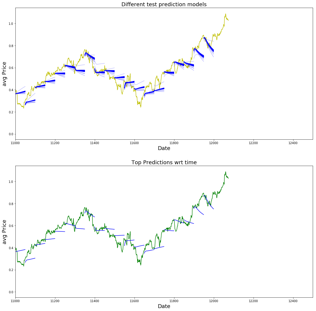

The cell picks one epoch as the representative "best" result and then draws two stacked plots that compare the true averaged price series to the model's test-time forecasts collected across training. The idea is to both show how the model's short-term forecasts evolved over epochs and to highlight the single epoch's predictions that looked best.

The top panel plots the full averaged price series as a yellow line over the date index, then overlays a sequence of blue prediction segments sampled from the recorded predictions over time. Only every third saved prediction set is drawn to reduce clutter, and an alpha envelope is applied so older prediction sets are semi-transparent while the more recent ones are more opaque. That fading effect is produced by ramping alpha from a low starting value up to full opacity across the sampled prediction-sets, so visually you can see a trail of light-blue, increasingly darker blue short forecast segments that track different test starting points along the time axis. The plotted blue segments are short because each saved prediction is a short autoregressive rollout beginning at a test anchor point; when drawn against the continuous yellow series you can see how each short forecast attempts to follow the immediate local trend.

The bottom panel repeats the true averaged price series in green and overlays the single set of predictions chosen by the bestpredictionepoch index in solid blue. This gives a cleaner view of what one strong epoch's forecasts looked like against the ground truth, without the layered transparency of the top panel. Both panels are focused on the same x-range so you can directly compare the evolution of predictions and where the best epoch sits in that progression.

The saved figure confirms this description: it contains two large axes, the top showing the yellow true series with many blue short-line forecast clusters fading from light to dark, and the bottom showing the green true series with the chosen epoch's blue prediction segments overlaid. The vertical scale sits around the normalized price range (roughly 0.2–1.1 in this run), and the short, angled blue strokes reflect the multi-step autoregressive predictions anchored at discrete test points rather than a continuous single-line forecast.

Conclusion

Tuning the model parameters and presenting the LSTM with sequential training examples instead of feeding it raw scalar prices led to noticeably better results. The network trained under these settings does not show signs of clear underfitting or overfitting.

Adjusting the batch size and applying the normalization procedure used during training made the task of forecasting short-term price movement much more tractable.

As a next step, adding external signals such as news or social media sentiment into the input has been reported to improve performance. Below are a few studies that combine sentiment information with historical prices for stock prediction:

Stock Movement Prediction from Tweets and Historical Prices by Yumo Xu and Shay B. Cohen
Stock Prediction Using Twitter Sentiment Analysis by Anshul Mittal and Arpit Goel
Sentiment Analysis for Effective Stock Market Prediction by Shri Bharthi and Angelina Geetha

Download source code using the button below: