Building Algorithmic Trading Strategies from First Principles EP:5/365

From Fama–French Factor Models to Momentum and Mean-Reversion Signals in Python

Download source code and dataset using the button at the end of this article!

This article walks through a complete, practical quantitative trading workflow, starting from how a tradable equity universe is constructed and ending with the evaluation of concrete algorithmic trading strategies. Rather than treating factor models or trading signals in isolation, it shows how the pieces fit together in a realistic research pipeline: sourcing data, handling survivorship bias, engineering factors, generating signals, and evaluating performance. The emphasis throughout is on clarity, reproducibility, and translating financial theory into code that can actually be tested.

The first part focuses on building an equity universe using ideas from the Fama–French five-factor model. It explains how market risk, size, value, profitability, and investment characteristics can be approximated using publicly available data, and how these characteristics help define and structure the investable universe. Along the way, the article demonstrates practical techniques such as caching data, aligning time series, and working with cross-sectional splits, all of which are essential for reliable quantitative research.

The second part shifts from factor construction to trading strategy design. It explores momentum, trend-following, and mean-reversion strategies, showing how intuitive market ideas translate into explicit trading rules. Each strategy is implemented step by step in Python, with careful attention to signal generation, order logic, and performance calculation. Both successful and unsuccessful strategies are discussed, highlighting why some commonly used approaches fail once tested rigorously.

By the end of the article, the reader will have a clear picture of how quantitative trading research is carried out in practice, from raw data to tested strategies. The goal is not to present a guaranteed profitable system, but to demonstrate a disciplined, transparent framework for developing, testing, and reasoning about algorithmic trading ideas in a way that mirrors real-world quant research.

Building an Equity Universe Using the Fama–French Five-Factor Model

import os
import numpy as np
import pandas as pd
import matplotlib.pyplot as plt
from tqdm import tqdm

import dotenv
%load_ext dotenv

import warnings
warnings.filterwarnings(”ignore”)

KAGGLE_FLAG = os.getenv(’IS_KAGGLE’, ‘True’) == ‘True’

if KAGGLE_FLAG:
    print(’Running in Kaggle...’)
    %pip install yfinance
    %pip install statsmodels
    %pip install seaborn
    %pip install itertools
    %pip install scikit-learn

    for root, _, file_list in os.walk(’/kaggle/input’):
        for file_name in file_list:
            print(os.path.join(root, file_name))
else:
    print(’Running Local...’)

import yfinance as yf
from analysis_utils import load_ticker_prices_ts_df as load_prices_ts_df, load_ticker_ts_df as load_ticker_ts_df

os.getcwd()

This block sets up the notebook environment and pulls in the libraries and helper functions you need to acquire, inspect, and work with time-series price data for quant trading tasks. It begins by loading environment variables via the dotenv notebook extension so that runtime configuration (like whether we are on Kaggle) can come from a .env file rather than being hard-coded. Warnings are then silenced to reduce console noise during exploratory runs; this keeps downstream output focused on the important messages and results when you fetch and analyze market data.

Next the code determines the runtime context by reading an environment variable named IS_KAGGLE. That value is compared to the string ‘True’ to produce a boolean flag (KAGGLE_FLAG). The flag controls a branching setup step: when running in a Kaggle kernel, the notebook explicitly installs several packages that are necessary for the remainder of the workflow — yfinance for market data pulls, statsmodels for statistical tests and time-series models, seaborn for richer plotting, itertools-related functionality for combinatoric operations used in e.g. pair selection, and scikit-learn for machine learning utilities. These installs are executed via notebook magics so the environment has the exact toolset required when the kernel starts from a minimal base image. After installing, the code enumerates all files under /kaggle/input and prints their full paths; that listing gives you immediate visibility into any preloaded datasets you can use for backtesting, feature construction, or cross-sectional analysis.

If the environment is not Kaggle, the else branch simply prints that the notebook is running locally. This branch assumes the local environment already contains the required libraries or that package management will be handled outside this snippet.

Finally, the script imports yfinance under the alias yf and pulls in two loader functions from a local analysis_utils module: load_ticker_prices_ts_df and load_ticker_ts_df. These helper functions are the bridge from raw data to the DataFrame structures you’ll use for quant analysis: typically they return time-indexed price series (adjusted closes, OHLC, or panel-like DataFrames) arranged per ticker, which are the starting point for signal generation, feature engineering, factor estimation, and backtesting. The call to os.getcwd() at the end simply inspects the current working directory, which helps confirm where relative paths and any subsequently loaded data files will be resolved during your quant workflows.

Factors

The model is built on five systematic risk factors that explain differences in asset returns. The first factor is the Market Risk Premium, denoted as MktRF, which represents the excess return of the overall market portfolio over the risk-free rate. The second factor is Size, captured by SMB (Small Minus Big), which measures the return difference between portfolios of small-cap firms and large-cap firms. The third factor is Value, represented by HML (High Minus Low), which reflects the return spread between firms with high and low book-to-market ratios. The fourth factor is Profitability, denoted by RMW (Robust Minus Weak), which captures the return difference between firms with strong operating profitability and those with weak profitability. The fifth and final factor is Investment, represented by CMA (Conservative Minus Aggressive), which measures the return difference between firms that invest conservatively and those that invest aggressively.

The relationship between these factors and asset returns is expressed through the following regression model:

In this equation, Rit​ denotes the return on asset iii at time ttt, while Rft​ is the risk-free rate at the same time. The term RMt​ refers to the return on the market portfolio, and the expression RMt​−Rft​ therefore represents the market risk premium, MktRF. The variables SMB, HML, RMW, and CMA correspond respectively to the size, value, profitability, and investment factor premiums at time ttt.

The parameter αi\alpha_iαi​ captures the asset-specific abnormal return that is not explained by the factors, while the β\betaβ coefficients measure the sensitivity of asset iii to each factor. The term ϵit\epsilon_{it}ϵit​ represents the error component, capturing idiosyncratic movements in returns that are not explained by the model.

Investable Universe

The investable universe refers to the set of assets for which this factor model is applied, typically consisting of publicly traded securities that satisfy liquidity, availability, and data-quality requirements.

import os
import pandas as pd
import yfinance as yf

START_DATE = “2003-01-01”
END_DATE = “2023-12-31”
DATA_DIR = “data”

uni_df = rf_df = None

csv_path = os.path.join(”.”, DATA_DIR, “S&P500_curated_historical_components.csv”)
sp500_df = pd.read_csv(csv_path)
sp500_df[”date”] = pd.to_datetime(sp500_df[”date”])
sp500_df = sp500_df[(sp500_df[”date”] >= START_DATE) & (sp500_df[”date”] <= END_DATE)]

tickers_list = sp500_df[”tickers”].str.split().explode().dropna().unique()
tickers = “ “.join(tickers_list)
assert len(tickers) > 0

cached_file_path = os.path.join(DATA_DIR, “cache”, “snp_comps.pkl”)
try:
    if os.path.exists(cached_file_path):
        equities_df = pd.read_pickle(cached_file_path)
    else:
        equities_df = yf.download(tickers, start=START_DATE, end=END_DATE, keepna=True)
        equities_df.to_pickle(cached_file_path)
except FileNotFoundError:
    print(f”Error downloading and caching or loading file”)

cached_file_path = os.path.join(DATA_DIR, “cache”, “t10.pkl”)
try:
    if os.path.exists(cached_file_path):
        rates_df = pd.read_pickle(cached_file_path)
    else:
        rates_df = yf.download(”^TNX”, start=START_DATE, end=END_DATE, keepna=True)[”Close”]
        rates_df.to_pickle(cached_file_path)
except FileNotFoundError:
    print(f”Error downloading and caching or loading file”)

uni_df, rf_df = equities_df, rates_df

uni_df, rf_df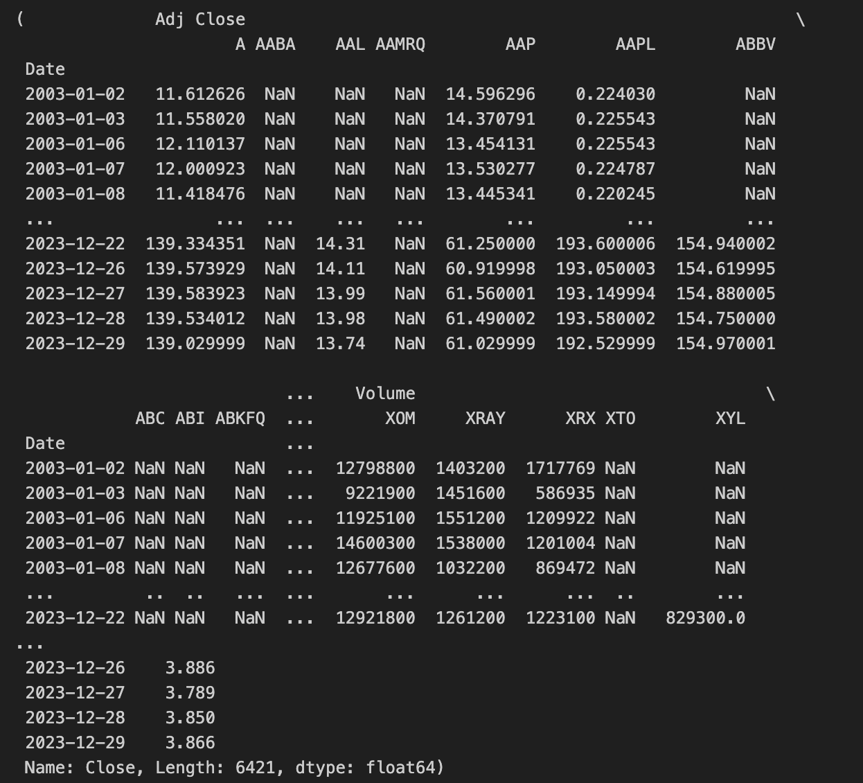

This block begins by loading a curated history of S&P 500 components from a CSV and immediately constraining it to the analysis window defined by START_DATE and END_DATE. The CSV is parsed so that the “date” column becomes a datetime indexable field, and then the frame is filtered to keep only rows whose dates fall into the two-decade span. The intent is to work only with components that were relevant during the chosen historical period so downstream price series and any universe construction align with the same temporal window.

From that filtered components table the code derives the universe of ticker symbols. Each row in the CSV contains a whitespace-delimited string of tickers; the code splits those strings, explodes them into a long series of one-ticker-per-row entries, drops any empty values, and takes the unique set. This yields a de-duplicated list of all tickers that appeared in the curated S&P composition within the target window. The list is then rejoined into a single space-separated string because the yfinance bulk download call accepts tickers provided in that format. An assertion ensures that the resulting string is non-empty so the download step has a valid set of symbols to request.

The equities download is protected by a simple file-cache pattern. A cached pickle path is constructed and, if that pickle exists, the code loads the pre-fetched DataFrame from disk to avoid re-querying the remote API. If the file is absent, it calls yfinance.download with the combined ticker string and the date bounds; the download response (which contains price fields for all tickers across the date range, typically as a multi-index column DataFrame) is then serialized to the same pickle path for future reuse. The keepna=True flag is passed to the download call so that missing observations are preserved as NaN rather than being dropped or implicitly forward-filled, which helps maintain alignment across tickers for subsequent cross-sectional or time-series calculations. The surrounding try/except only prints a simple message if a FileNotFoundError is raised during the load/cache operations.

A parallel cache-and-download flow is applied to obtain a risk-free proxy: the 10-year Treasury yield series identified by yfinance ticker “^TNX”. The code checks for a cached pickle and otherwise downloads the series over the same START_DATE/END_DATE window. After downloading, it explicitly selects the “Close” column from the returned data so that rates_df becomes a single time series of daily closing yields. This series is intended to serve as the risk-free rate input (rf_df) for return calculations, discounting, or other fixed-income referenced metrics used in quant trading strategies.

Finally, the two downloaded objects are mapped into the names expected by downstream quant pipeline code: uni_df receives the equities DataFrame and rf_df receives the rates series. The block returns these two datasets (uni_df, rf_df) so the rest of the strategy stack can compute returns, perform portfolio construction, factor regressions, signal generation, or any backtesting steps that require synchronized equity prices and a benchmark risk-free series. Overall, the sequence ensures the universe is temporally consistent with the curated S&P composition, preserves missing data for alignment, and uses on-disk caching to make repeated experimentation efficient.

Market Risk Factor

t_df = None
ticker_names = uni_df.columns.get_level_values(1).unique()
cache_file = f”{DATA_DIR}/cache/snp_comps_hist.pkl”
try:
    tickers_client = yf.Tickers(” “.join(ticker_names))
    t_df = tickers_client
    if os.path.exists(cache_file):
        t_hist_df = pd.read_pickle(cache_file)
    else:
        downloaded_hist = tickers_client.history(start=START_DATE, end=END_DATE)
        downloaded_hist.to_pickle(cache_file)
        t_hist_df = downloaded_hist
except FileNotFoundError:
    print(f”Error downloading and caching or loading file”)

t_hist_df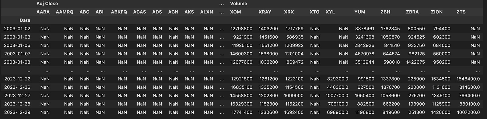

This block is responsible for assembling a historical price dataset for a list of tickers (the S&P components in this context), caching it locally, and exposing both the live yf.Tickers client and the historical DataFrame for downstream quant workflows. It starts by pulling the ticker identifiers from a MultiIndex columns object (uni_df.columns.get_level_values(1).unique()); taking the second level and then unique() ensures we get a deduplicated list of ticker symbols that represent the universe we want to analyze. Those symbol strings are then concatenated into a single space-separated string because the yfinance.Tickers constructor accepts multiple tickers in that format.

Next the code composes a cache path in DATA_DIR/cache named snp_comps_hist.pkl. Inside the try block it instantiates the yfinance Tickers client with the concatenated ticker string and stores that object in t_df so the client reference is kept available (useful for any later live queries or metadata access). The key decision point is whether to reuse a previously saved cache: if the pickle file exists, the code loads the historical DataFrame directly with pd.read_pickle and assigns it to t_hist_df, which avoids network traffic and yields a reproducible, disk-backed snapshot of historical prices. If the cache file is not present, the code calls tickers_client.history(start=START_DATE, end=END_DATE) to download the full OHLCV time series for the requested date range, immediately writes that downloaded DataFrame out to the same pickle path with to_pickle, and then sets t_hist_df to the freshly downloaded DataFrame. In both branches t_hist_df ends up containing the same logical dataset: the historical time series for all tickers, typically organized by timestamp index and with per-ticker price/volume columns as produced by yfinance.

A FileNotFoundError is caught around the whole download/read/cache sequence; if such an exception occurs the code prints a simple error message. Finally, the last expression evaluates t_hist_df so the resulting historical DataFrame is returned from this block for use in feature construction, signal generation, backtests, or other quant trading tasks that rely on historical price and volume series.

cap_map = {}
pb_map = {}
opm_map = {}
roa_map = {}

cached_file_path = f”{DATA_DIR}/cache/fund_snp500.pkl”
try:
    if os.path.exists(cached_file_path):
        fund_df = pd.read_pickle(cached_file_path)
    else:
        for ticker in tqdm(tickers):
            try:
                if (info := t_df.tickers[ticker].info) is None:
                    continue
                cap_map[ticker] = info.get(”marketCap”, np.nan)
                pb_map[ticker] = info.get(”priceToBook”, np.nan)
                opm_map[ticker] = info.get(”operatingMargins”, np.nan)
                roa_map[ticker] = info.get(”returnOnAssets”, np.nan)
            except Exception as e:
                print(f”Error processing ticker {ticker}: {e}”)

        fund_df = pd.DataFrame(
            {
                “MarketCap”: pd.Series(cap_map),
                “PriceToBook”: pd.Series(pb_map),
                “OperatingMargins”: pd.Series(opm_map),
                “ReturnOnAssets”: pd.Series(roa_map),
            }
        )
        fund_df.to_pickle(cached_file_path)
except FileNotFoundError as fnf_error:
    print(f”File not found error: {fnf_error}”)
except Exception as e:
    print(f”Error downloading and caching or loading file: {e}”)

This block builds and caches a small fundamentals table for a universe of tickers so downstream quant routines can use consistent, quickly accessible feature columns. At the top we create four plain dictionaries keyed by ticker: cap_map, pb_map, opm_map, and roa_map. Those maps will hold market capitalization, price-to-book, operating margin, and return-on-assets respectively — basic value and profitability metrics that commonly serve as features or filters in quantitative strategies.

The code then computes a cache path and enters a guarded flow: if a pickle already exists at that path, it is loaded directly into fund_df with pd.read_pickle. This avoids repeatedly hitting the data source and provides deterministic input for backtests or model training. If the cache is not present, the code iterates over the tickers (with tqdm to report progress) and pulls each ticker’s metadata from t_df.tickers[ticker].info. For each ticker, it first skips any entries where info is None, and otherwise extracts the four named fields using dict.get with np.nan as the default. Using np.nan explicitly preserves missingness in a numeric-friendly form so later numeric operations, imputation, or filters can handle missing values consistently.

The per-ticker extraction is wrapped in a try/except so a failure on one ticker (for example due to an intermittent API/attribute error) prints an error but does not terminate the whole collection process; this ensures you still build a usable table from the remaining tickers. After the loop completes, those four maps are converted into pandas Series and assembled into a DataFrame with columns MarketCap, PriceToBook, OperatingMargins, and ReturnOnAssets. Constructing the DataFrame from Series built from the dictionaries naturally aligns rows by ticker symbols (the dictionary keys become the index), giving a tidy, indexed DataFrame where each row corresponds to a ticker.

Finally, once the DataFrame is constructed it is written out to the same pickle path using fund_df.to_pickle so subsequent runs can load the cached file instead of re-querying the source. The entire outer operation is wrapped in an exception handler that specifically prints FileNotFoundError messages and also captures any other exceptions with a general message, so file-system or other unexpected problems are surfaced without producing silent failures. Overall, the block’s data flow is: attempt to load cached fundamentals → if missing, iterate tickers to collect selected fundamental metrics into maps → assemble aligned DataFrame from those maps → persist the result for fast reuse in quant workflows.

fund_df.__getitem__(”MarketCap”)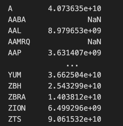

This single call invokes the DataFrame’s column-access machinery to extract the column labeled “MarketCap” from fund_df and return it as a one-dimensional pandas Series. Internally this is the same operation performed by the more common fund_df[“MarketCap”] bracket syntax: pandas looks up the column label in the DataFrame’s columns, pulls out the underlying values for every row, assigns the Series the same index as the parent DataFrame, and preserves the column name and dtype on the returned object.

From a data-flow perspective, this line takes the table of fund-level metrics and isolates the market-capitalization vector so subsequent code works with per-asset market-cap values rather than the full multi-column table. Because the Series retains the DataFrame’s index, any later alignment, merging, or index-aware arithmetic will stay consistent with the original rows (for example, matching timestamps or tickers).

In the context of quant trading, extracting MarketCap is typically done so you can feed those capitalization figures into sizing and risk decisions: constructing cap-weighted portfolios, computing size-based factor ranks, filtering out small-cap liquidity risks, or normalizing exposures by market size. This call is the explicit step that turns the column from a table field into a standalone numeric vector ready for those downstream calculations.

market_caps = fund_df[”MarketCap”]
total_market_cap = market_caps.sum()
weights = market_caps.div(total_market_cap)

adj_close_prices = uni_df[”Adj Close”]
period_returns = adj_close_prices.pct_change()
weighted_market_series = (period_returns * weights).sum(axis=1)
average_market_return = weighted_market_series.mean()

rm_rf_series = average_market_return - rf_df

rm_rf_series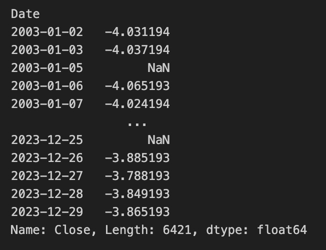

This block constructs a market portfolio return and then produces a time series measuring that market return in excess of the risk-free rate — essentially the market risk premium factor used in quant trading and factor models.

First, the code extracts each asset’s market capitalization and normalizes those values into weights by dividing each market cap by the total market cap. The intent here is to create a market-cap-weighted portfolio: the normalization ensures the weights sum to one so each asset’s influence on the portfolio return is proportional to its relative market size.

Next, the code computes simple period returns from adjusted close prices via a percentage change. That yields a DataFrame of per-period returns for each asset, indexed by date. These per-asset returns are then multiplied by the weights Series; because the weights are aligned by asset labels, this multiplies each asset’s return time series by its corresponding market weight, producing a weighted return contribution for every asset and date. Summing across columns (sum with axis=1) aggregates those contributions into a single time series of the market-cap-weighted portfolio return for each period.

The weighted_market_series is then reduced to a single scalar average_market_return by taking its mean across time. This step converts the time series of periodic market returns into an overall average return across the sample window — effectively a single expected market return estimate computed as the sample mean of the weighted portfolio returns.

Finally, the code subtracts the risk-free rate series (rf_df) from that scalar average. Because average_market_return is a scalar and rf_df is a time series indexed by date, the subtraction yields a date-indexed Series where each entry equals the same average market return minus the risk-free rate at that date. The resulting rm_rf_series therefore represents, for each date, the difference between the long-run average market return and the contemporaneous risk-free rate — a form of market excess return series used downstream in quant models.

Size (Risk Factor)

from tqdm import tqdm

for _date, _df in tqdm(uni_df.items()):
    median_val = mrk_cap.median()
    tmp_small = mrk_cap[mrk_cap < median_val]
    tmp_big = mrk_cap[mrk_cap >= median_val]

small_companies, big_companies = tmp_small, tmp_big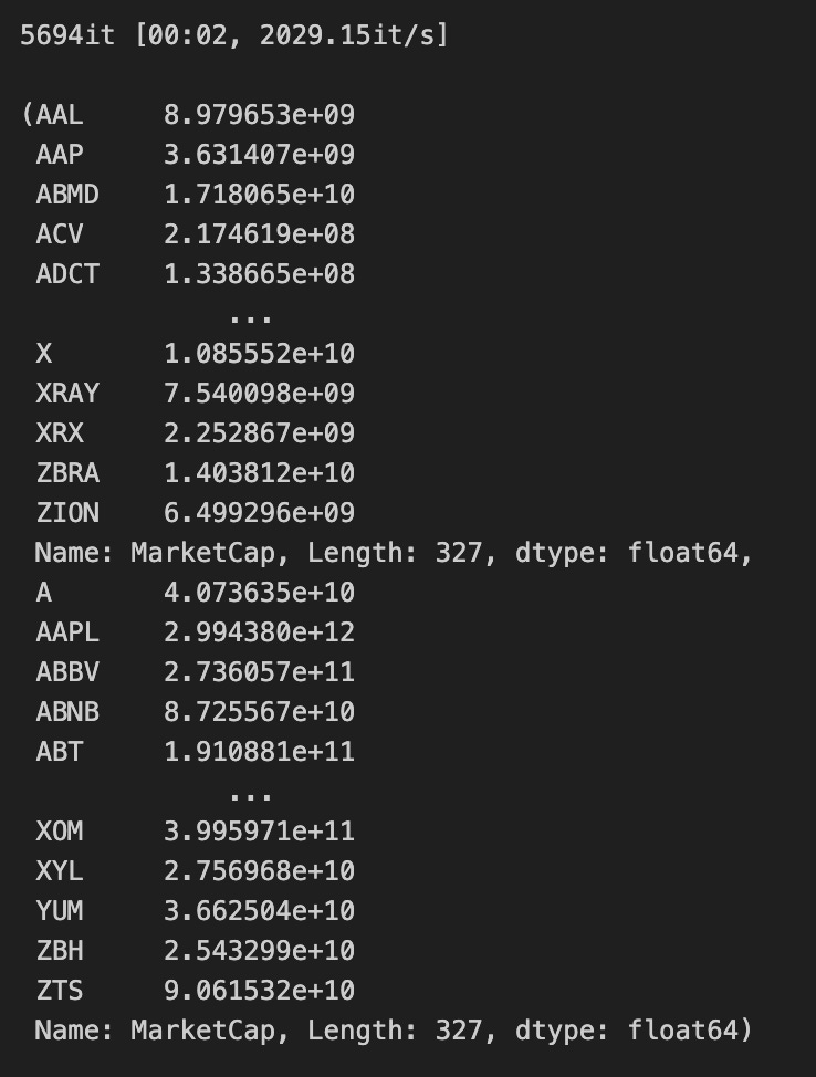

The outer structure is a straightforward, progress-tracked iteration over uni_df.items() — tqdm wraps the iterator so you get a progress bar as the loop runs. Each iteration yields a key/value pair (_date, _df); the variable names use a leading underscore to indicate the loop doesn’t use them directly in the body, but the loop itself still drives repeated execution of the inner logic for as many entries as uni_df contains.

Inside the loop the code computes median_val = mrk_cap.median() and then slices mrk_cap into two subsets: tmp_small contains the entries whose market capitalization is strictly less than the median, and tmp_big contains those whose market capitalization is greater than or equal to the median. Conceptually this is a binary partition of the universe into “small” and “big” buckets based on the central tendency of market cap; the median split ensures roughly half the names fall into each side, which is useful in quant trading when you want balanced groups for size-based factor analysis, portfolio construction, or comparative performance measurement.

Because the median and the two slices are computed from the mrk_cap object, the actual content of tmp_small and tmp_big at each loop pass depends entirely on the state of mrk_cap at that moment. Each iteration overwrites tmp_small and tmp_big with the freshly computed slices, so when the loop finishes the variables contain the results produced by the final iteration.

After the loop, small_companies and big_companies are assigned the last computed tmp_small and tmp_big respectively. In other words, the script exposes the final median-based partition of mrk_cap as small_companies and big_companies for downstream use in the quant workflow (e.g., constructing size buckets, computing size-premium returns, or conditioning other signals on company size).

Value: Risk Factor

price_to_book = fund_df[”PriceToBook”]
median_val = price_to_book.quantile(0.5)
lower_group = price_to_book[price_to_book < median_val]
higher_group = price_to_book[price_to_book >= median_val]
higher_group, lower_group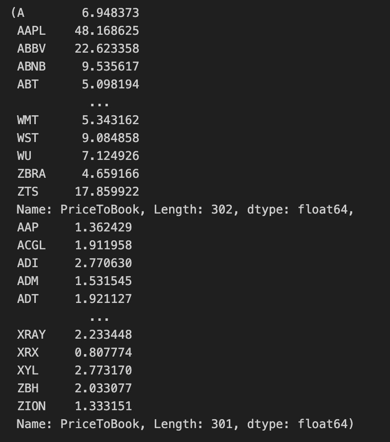

This snippet takes a column of Price-to-Book ratios from a DataFrame and partitions that cross-section into two cohorts around the median valuation to support downstream quant trading tasks (e.g., constructing low- vs. high-valuation portfolios or generating a binary value signal).

First, the code extracts the PriceToBook series from fund_df so subsequent operations work on the per-asset valuation signal. It then computes the median of that series with quantile(0.5), which yields a single threshold value (median_val) representing the 50th percentile of the available Price-to-Book observations. Using the median as the threshold is a deliberate choice to split the cross-section down the middle in a way that is robust to extreme outliers in the distribution.

Next, two boolean filters are applied to create the cohorts. lower_group selects all entries strictly less than the median (price_to_book < median_val), while higher_group selects all entries greater than or equal to the median (price_to_book >= median_val). Because the selection is performed by indexing the original Series with boolean masks, each resulting group remains a pandas Series that preserves the original index labels, which keeps the link back to other asset attributes for any subsequent merging, ranking, or portfolio construction steps.

Finally, the expression returns a tuple in the order (higher_group, lower_group). In the context of a quant workflow this produces two labeled cross-sectional universes — one representing the higher-or-equal median Price-to-Book assets and one representing the strictly lower-than-median assets — ready for use in constructing long/short legs, computing group-level statistics, or feeding into performance attribution pipelines.

Profitibility Risk

margins_series = fund_df.loc[:, “OperatingMargins”]
median_value = margins_series.quantile(0.5)
below_median = margins_series[margins_series.lt(median_value)]
at_or_above_median = margins_series[margins_series.ge(median_value)]

at_or_above_median, below_median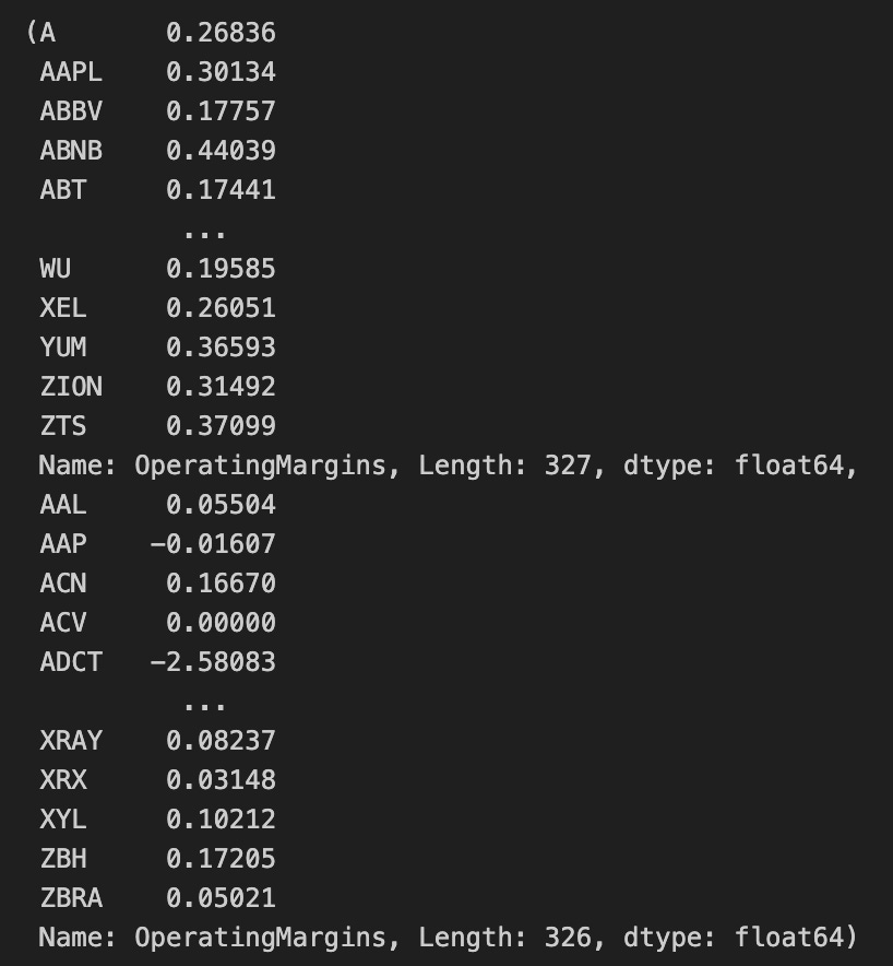

This snippet is performing a simple, deterministic split of the operating-margin data into two groups around the median to support downstream quant trading decisions (for example, treating firms with stronger operating margins differently from weaker ones in signal construction or portfolio tilting). The code first extracts the operating-margins column from the DataFrame as a Series so that subsequent operations act on a one-dimensional array of margin values indexed by the original identifiers; working with a Series preserves index alignment for later merging or scoring steps.

Next, the code computes the 0.5 quantile of that Series to obtain the sample median. Using the quantile method produces the statistical median of the available values (quantile ignores NaNs when computing the result), which provides a robust central threshold that is less sensitive to extreme outliers than a simple mean would be. The median therefore serves as a stable cutoff to partition the universe into lower- and higher-margin groups for signal generation or risk profiling.

With the median in hand, the Series is split into two new Series via boolean masking. The first mask selects values strictly less than the median (margins_series.lt(median_value)) and yields a Series of all observations below the median; the second mask selects values greater than or equal to the median (margins_series.ge(median_value)) and yields the other group. Because lt and ge return boolean masks aligned to the original index, the resulting subsets retain their original row labels and can be directly compared, joined, or ranked against other factor Series.

Finally, the code returns a tuple with the at-or-above-median Series first and the below-median Series second. Note that values exactly equal to the computed median are included in the at-or-above group due to the use of ge, so the partition is strictly “below median” versus “median or above.” This split creates two keyed buckets of firms that can be used downstream in the quant workflow (e.g., bucketed exposures, group-wise statistics, or conditional signal application).

Investment Risk Factor

A characteristic that contributes to an investment’s potential for loss.

asset_returns = fund_df[”ReturnOnAssets”]
median_value = asset_returns.quantile(0.5)
conservative_companies = asset_returns.loc[asset_returns < median_value]
aggressive_companies = asset_returns.loc[asset_returns >= median_value]
conservative_companies, aggressive_companies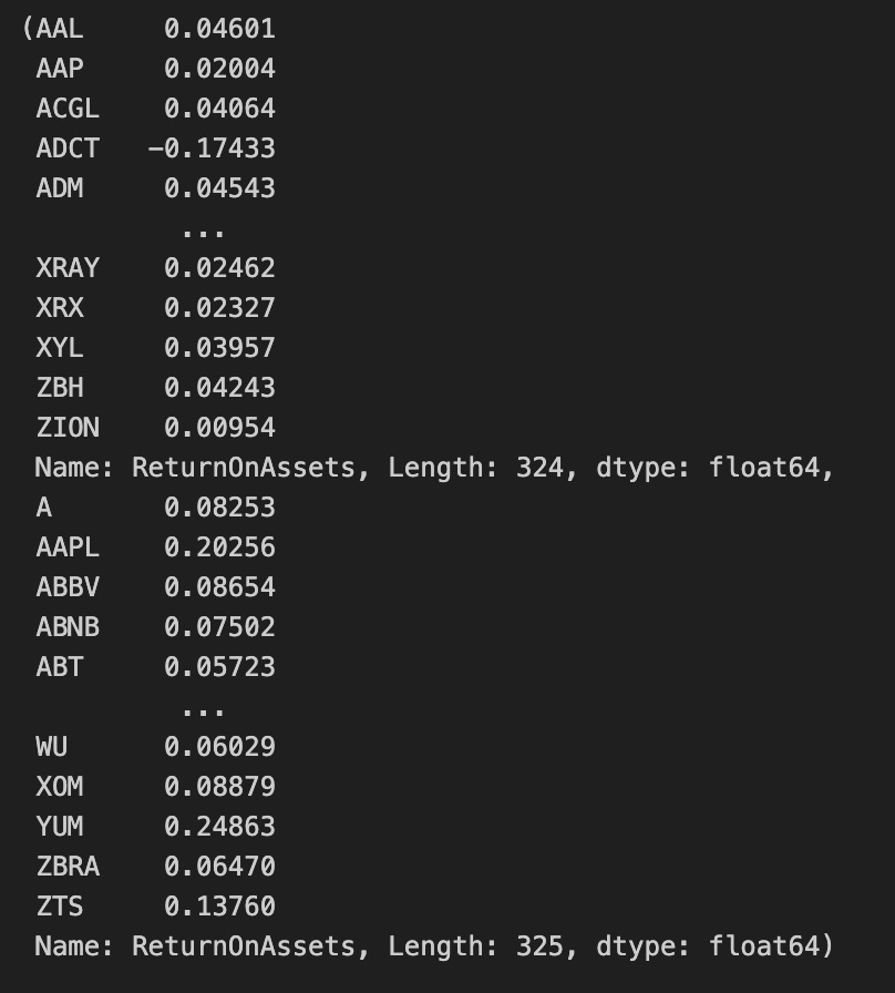

The first line pulls the “ReturnOnAssets” column out of the fund-level DataFrame into a one-dimensional series of asset return metrics; think of this series as the universe of firms represented by a single, comparable profitability metric. The next line computes the 50th percentile (the median) of that series, producing a single threshold value that splits the observed distribution into two equal-probability halves. Using the median rather than a mean is intentional here: the median provides a non-parametric, outlier-robust cutpoint so the split is less sensitive to extreme ROA values.

With the threshold in hand, the code creates two subset series. conservative_companies selects all entries whose ROA is strictly less than the median, so it captures the lower half of the distribution; aggressive_companies selects entries whose ROA is greater than or equal to the median, which places any firms exactly at the median into the aggressive group. Both subsets preserve the original index and values from the ROA series, so you retain firm identifiers and raw metric values for downstream use. The final expression simply returns the pair of series as a tuple.

In the context of quantitative trading, this sequence implements a simple signal-based segmentation: it classifies the investment universe into lower-ROA (“conservative”) and higher-ROA (“aggressive”) cohorts using a robust central tendency cutoff. Those cohorts can then be treated as separate buckets for strategy construction, backtests, performance attribution, or risk assessment, with the ROA threshold serving as the deterministic rule that governs group membership.

---

Analysis of Momentum and Reversion Trading Signals

In quantitative trading, a variety of strategies are used to seek an edge in financial markets. Two of the most widely used approaches are trend-following and momentum; because they are broadly adopted, they generally offer limited alpha for most practitioners.

Momentum and trend approaches both exploit persistence in price behavior, but they differ in emphasis:

- Trend-following targets directional, absolute returns and typically considers market beta across the broader market.

- Momentum targets relative returns and is often implemented in a market-neutral way, comparing assets within a class or sector cross-section.

Reversion refers to the assumption that prices will revert to a mean (or to one of several means) over time.

This article analyzes these strategies and provides Python implementations you can run yourself. We will progress toward more advanced methods and analyses — see Pairs Trading for a related example.

The analysis focuses on the post-pandemic market regime, so most price series begin in 2021. All strategies discussed are long-only and unleveraged.

import os
import dotenv
%load_ext dotenv

import warnings
warnings.filterwarnings(”ignore”)

import numpy as np
import pandas as pd
import matplotlib.pyplot as plt

is_running_on_kaggle = os.getenv(’IS_KAGGLE’, ‘True’) == ‘True’

if is_running_on_kaggle:
    print(’Running in Kaggle...’)
    %pip install yfinance

    for dirpath, _, file_list in os.walk(’/kaggle/input’):
        for file_name in file_list:
            print(os.path.join(dirpath, file_name))
else:
    print(’Running Local...’)

import yfinance as yf
from analysis_utils import calculate_profit, load_ticker_ts_df, plot_strategy

The first part of the block sets up the notebook execution environment and common scientific libraries used for time-series analysis. It activates dotenv support so environment variables from a .env file can be loaded into the process, and it imports numpy, pandas and matplotlib because they provide the numerical arrays, tabular data structures and plotting primitives that any quant workflow depends on. Warnings are explicitly suppressed so that non-critical library warnings don’t clutter notebook output during data downloads, calculations and plotting; the intent is to keep the output focused on the trading analysis results.

Next, the code determines whether it is running inside the Kaggle execution environment by reading the IS_KAGGLE environment variable and comparing it to the string ‘True’, defaulting to ‘True’ when the variable is not set. This boolean drives environment-specific behavior: in a hosted notebook environment like Kaggle you often need to both ensure required libraries are available and discover dataset files that have been uploaded to the kernel, whereas in a local environment those steps are unnecessary or handled differently.

When the code detects Kaggle, it prints a short message, then uses the notebook pip magic to install yfinance at runtime so the subsequent data-fetching calls will work. It then walks the /kaggle/input directory and prints full paths for every file it finds; this is a practical discovery step so the analyst or downstream code can see which historical datasets or supplemental files were made available to the kernel and therefore which asset histories or configuration files can be loaded for backtesting and analysis.

If not running on Kaggle, the code simply prints that it’s running locally and skips the installation and dataset-discovery steps. That branch keeps local runs lean where installation and data provisioning are expected to be managed by the developer rather than the notebook environment.

Finally, the code imports yfinance (the library used to fetch historical market data from Yahoo Finance) and three functions from analysis_utils: calculate_profit, load_ticker_ts_df, and plot_strategy. These imports indicate the next stage of the workflow: fetching or loading price time series, computing strategy profit metrics, and producing visualizations of the trading strategy performance. Together, the conditional setup plus these imports prepare the notebook to load market data, run backtests, and visualize outcomes — core activities in quantitative trading workflows.

Momentum & Trend Strategies

Consider an example: if an asset’s price has risen over the past week, it is likely to continue rising. Momentum and trend strategies rely on the assumption that recent price behavior tends to persist, producing sustained upward or downward trends. As some online traders quipped, “stonks only go up.”

Although straightforward to understand and implement, these strategies have several drawbacks:

- They can smooth or obscure important price moves by ignoring market noise and idiosyncratic events.

- Frequent trades can generate significant transaction costs.

- Because the approach is widely used, it may offer limited edge.

We will implement several of these strategies.

Simple Moving Average (SMA) Crossover

The moving average crossover strategy computes two moving averages of the asset’s price: a short-term (fast) SMA and a long-term (slow) SMA.

The code below implements this strategy:

import pandas as pd
import numpy as np

def double_simple_moving_average_signals(ticker_ts_df, short_window=5, long_window=30):
    # Build result frame with same index
    result = pd.DataFrame(index=ticker_ts_df.index)
    result[’signal’] = 0.0

    prices = ticker_ts_df[’Close’]
    short_sma = prices.rolling(window=short_window, min_periods=APO_FAST_WINDOW, center=False).mean()
    long_sma = prices.rolling(window=long_window, min_periods=APO_FAST_WINDOW, center=False).mean()

    result[’short_mavg’] = short_sma
    result[’long_mavg’] = long_sma

    # 1 when short SMA exceeds long SMA, else 0
    result[’signal’] = (short_sma > long_sma).astype(float)

    result[’orders’] = result[’signal’].diff()
    result.loc[result[’orders’] == 0, ‘orders’] = None

    return result

This function implements a classic short/long simple moving average (SMA) crossover rule to produce time-aligned trading signals and discrete order events from a ticker time series — the kind of lightweight trend-following logic commonly used as an entry/exit rule in quant trading strategies.

First, the function creates a result DataFrame that preserves the original timestamp index so every signal aligns exactly with the input market bars. It initializes a numeric ‘signal’ column to 0.0 so there is a well-defined default state (flat/no-long) for every timestamp before the moving-average logic runs.

Next it extracts the price series (Close) and computes two rolling means: a short-term SMA over short_window bars and a long-term SMA over long_window bars. Both rolling calls use the specified min_periods parameter (APO_FAST_WINDOW in this code) and center=False, which means each SMA value is computed from the current bar and the preceding bars up to the window length — this aligns the indicator to the time the information would actually be available in a live system. The short and long SMAs are stored back into the result frame as ‘short_mavg’ and ‘long_mavg’ so the rule’s inputs are kept with the signals for inspection or backtesting.

The function then implements the binary crossover rule: it sets ‘signal’ to 1.0 wherever the short SMA strictly exceeds the long SMA, and to 0.0 otherwise. Converting the boolean comparison to float yields explicit numeric signals that are convenient for arithmetic and differencing.

To translate state changes into discrete trade events, it computes ‘orders’ as the first difference of the ‘signal’ series. This produces +1.0 when the signal transitions from 0 to 1 (a buy/enter-long event), -1.0 when it transitions from 1 to 0 (a sell/exit-long event), and 0.0 for time steps where the state is unchanged. The code then replaces those zero differences with None, leaving the column populated only at timestamps where an actual order event occurred; unchanged-state rows are explicitly marked as non-events. Finally, the function returns the result DataFrame, which contains timestamps, the two moving averages, the current binary position signal (0.0 or 1.0), and sparse order markers indicating the discrete entry or exit events derived from the SMA crossover.

This function accepts a stock time series, computes short (fast SMA) and long (slow SMA) rolling windows, and compares them over time. It emits a buy signal (1) when the fast SMA exceeds the slow SMA, and a sell signal (-1) when the fast SMA is lower.

Execute all steps at once:

import matplotlib.pyplot as plt

ticker = ‘AAPL’
start_date, end_date = ‘2021-01-01’, ‘2023-01-01’

apple_ts_df = load_ticker_ts_df(ticker, start_date=start_date, end_date=end_date)
signal_df = double_simple_moving_average_signals(apple_ts_df, 5, 30)
profit_series = calculate_profit(signal_df, apple_ts_df[”Adj Close”])
ax1, ax2 = plot_strategy(apple_ts_df[”Adj Close”], signal_df, profit_series)

mavg_columns = [(’short_mavg’, ‘Fast SMA’), (’long_mavg’, ‘Slow SMA’)]
for col, lbl in mavg_columns:
    ax1.plot(signal_df.index, signal_df[col], linestyle=’--’, label=lbl)

ax1.legend(loc=’upper left’, fontsize=10)
plt.show()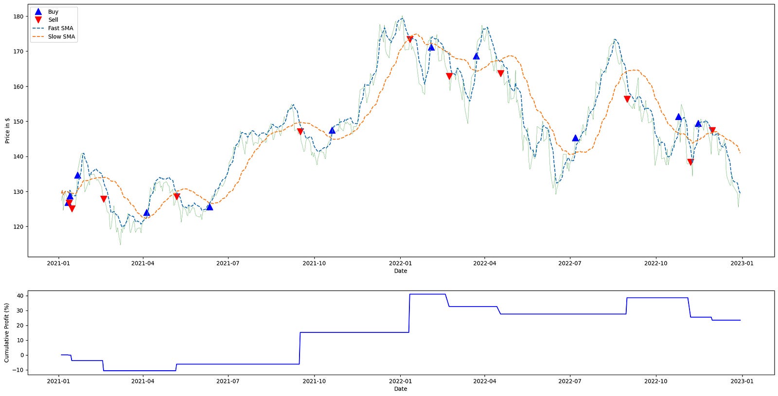

The code begins by defining the universe and time window for analysis: the ticker symbol and start/end dates constrain the historical price series that will drive the strategy. That price series is fetched into apple_ts_df via load_ticker_ts_df; within the quant-trading context this DataFrame is the canonical source of market data (including an “Adj Close” column), and using adjusted close prices ensures that returns and signals reflect corporate actions like splits and dividends so performance calculations are meaningful and comparable over time.

Next, double_simple_moving_average_signals is applied to the time series with windows 5 and 30. Conceptually this computes two simple moving averages (a short/fast average with period 5 and a long/slow average with period 30) and produces a signal frame that encodes the crossovers between them. The reason for the SMA crossover structure is that crossing relationships between a fast and slow moving average are used to infer short-term trend changes: when the short SMA crosses above the long SMA you typically enter or hold a long exposure, and when it crosses below you exit or take neutral/short exposure. The signal_df therefore contains the moving-average columns (e.g., short_mavg, long_mavg) plus the discrete or continuous position indicator(s) that the trading logic uses downstream.

calculate_profit then consumes those signals together with the adjusted-close price series to produce profit_series. This function aligns the trading signals with actual execution prices and converts those position signals into a time series of realized or mark-to-market profit (period returns or cumulative P&L), which is the numeric measure of strategy performance. The ordering matters: we generate signals from market data first, and only then translate signals into profits by applying them to the same adjusted close prices, ensuring the performance trace corresponds precisely to the signal decisions.

plot_strategy takes the price series, the signal frame, and the computed profit series and produces two plotting axes (ax1, ax2). In practice ax1 is used to show the price path and trade markers or position overlays, and ax2 is used to visualize performance metrics such as cumulative returns or profit over time. Returning the axes rather than immediately showing the plot gives the caller the ability to augment those axes with additional lines or annotations; here the code uses that capability to overlay the two SMA lines onto the price axis for visual confirmation of the crossover logic.

The loop over mavg_columns walks the pairings of column name and human-readable label and draws each moving average from signal_df onto ax1 with a dashed linestyle and the provided label. Plotting these SMAs on the same axis as price lets you visually correlate where crossovers occur relative to price action, making it easier to interpret why specific entries and exits happened and how they contributed to the profit_series. Finally, ax1.legend(…) places a legend on the price axis so the SMA labels are visible, and plt.show() renders the combined plot, giving a single visual summary that ties the raw price, the moving averages that generated signals, and the strategy’s profit trace together for evaluation in the quant-trading workflow.

Over two years, this strategy delivered a 30% return, significantly outperforming the S&P 500, which returned 10%.

Naive Momentum

This strategy counts consecutive price increases or decreases. It assumes that a price that rises for a certain number of consecutive days is a buy signal, and that a price that falls for the same number of consecutive days is a sell signal. We will reuse some of the utility functions from the SMA strategy above.

Below is a simple implementation:

def naive_momentum_signals(ticker_ts_df, nb_conseq_days=2):
    signals = pd.DataFrame(index=ticker_ts_df.index)
    signals[’orders’] = 0

    adj_close = ticker_ts_df[’Adj Close’]
    diffs = adj_close.diff()

    current_signal = 0
    streak = 0

    for pos in range(1, len(ticker_ts_df)):
        delta = diffs.iat[pos]
        if delta > 0:
            streak += 1
            if streak == nb_conseq_days and current_signal != 1:
                signals[’orders’].iat[pos] = 1
                current_signal = 1
        elif delta < 0:
            streak -= 1
            if streak == -nb_conseq_days and current_signal != -1:
                signals[’orders’].iat[pos] = -1
                current_signal = -1

    return signals


signal_df = naive_momentum_signals(aapl_ts_df)
profit_series = calculate_profit(signal_df, aapl_ts_df[”Adj Close”])
ax1, _ = plot_strategy(aapl_ts_df[”Adj Close”], signal_df, profit_series)

ax1.legend(loc=’upper left’, fontsize=10)
plt.show()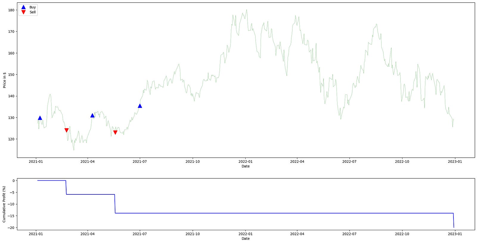

This function implements a simple, rule-based momentum entry signal generator intended for use in a quant trading workflow: it looks for runs of consecutive days in which the adjusted close moves in the same direction and emits a single order when a run reaches a configured length. The overall flow is: compute day-to-day price changes, maintain a running signed “streak” count that grows or shrinks as the price moves up or down, and when that streak exactly equals the configured threshold emit either a long (+1) or short (-1) order for that day. The produced signals DataFrame is then handed off to a profit-calculation routine and a plotting helper to visualize strategy performance against the underlying adjusted close series.

Internally, the function creates an aligned signals DataFrame with an “orders” column initialized to zeros so every index in the input time series has a corresponding spot for an order. It extracts the “Adj Close” series and computes simple first differences (adj_close.diff()) to capture the sign and magnitude of daily moves; these differences are used only for sign/direction decisions here, i.e., whether the day was up (delta > 0), down (delta < 0), or flat (delta == 0). Two state variables drive the decision logic as the loop iterates through each day starting from the second row (pos = 1): streak tracks the cumulative signed run-length of consecutive ups or downs, and current_signal records the last active position state (0 = flat/no position, 1 = long, -1 = short). Iteration begins at 1 to avoid the NaN difference at the series start and to align the order assignment with the day on which the threshold is reached.

Within the loop the code updates streak and decides whether to emit an order. On an up day (delta > 0) the streak is incremented; once the streak exactly equals nb_conseq_days and the current position state is not already long, the function records a +1 order at that day’s index and sets current_signal to 1. Conversely, on a down day (delta < 0) the streak is decremented; when it exactly equals -nb_conseq_days and the current position state is not already short, the function records a -1 order and sets current_signal to -1. Flat days (delta == 0) leave streak unchanged and therefore do not trigger any order activity. Because the code checks current_signal before writing an order, it emits a single order when a qualifying streak is first reached and avoids writing repeated identical orders on subsequent days of the same trend. Note also that the streak is signed and accumulates across direction changes (positive increments for up days, negative decrements for down days) rather than being reset to zero on a sign flip; an explicit order is emitted only when the streak crosses exactly to the +nb_conseq_days or -nb_conseq_days value.

After the loop completes, the function returns the signals DataFrame with a sparse set of +1 / -1 entries at the indices where entries into long or short positions are signaled. In the usage shown, that returned signal_df is passed with the adjusted close series into calculate_profit to produce a profit_series that reflects hypothetical P&L from following those entry signals, and into plot_strategy to render the price series, the signals, and the profit trace. The plotting call returns an axis (ax1) that receives a legend placed in the upper-left; finally plt.show() displays the composite figure so you can visually inspect where the naive momentum entries occurred and how the strategy performed over time.

This strategy was unprofitable and generated no returns. We would have achieved better results by inverting the model — as is often advisable with much of WSB’s stock analysis. To invert the signals, use: `signals[‘orders’] = signals[‘orders’] * -1`.

Note that this approach is typically applied to the broader market rather than a single instrument and is usually executed over a shorter time frame.

Reversion Strategies

Example: Elon tweets that he will install blockchain in Teslas, and the market becomes overzealous in buying Tesla stock. The next day, when participants realize that the underlying fundamentals have not changed, interest fades and the price reverts to a more appropriate level.

Therefore, any instrument that diverges too quickly from a benchmark in either direction will typically revert over a longer timeframe.

Like trend and momentum approaches, mean reversion is a simple strategy that smooths short-term noise and is generally used by market participants.

Mean Reversion

Here we assume that a stock’s price will remain in the vicinity of its mean.

Below is the signal code:

import pandas as pd
import numpy as np

def mean_reversion_signals(ticker_ts_df, entry_threshold=1.0, exit_threshold=0.5):
    idx = ticker_ts_df.index
    prices = ticker_ts_df[’Adj Close’]
    window = 20

    rolling_mean = prices.rolling(window).mean()
    rolling_std = prices.rolling(window).std()

    result = pd.DataFrame(index=idx)
    result[’mean’] = rolling_mean
    result[’std’] = rolling_std

    # Final signal mirrors original behavior (downside condition overrides)
    signal_arr = np.where(prices < (rolling_mean - exit_threshold * rolling_std), -1, 0)
    result[’signal’] = signal_arr

    orders_series = pd.Series(signal_arr, index=idx).diff()
    orders_series = orders_series.mask(orders_series == 0, None)
    result[’orders’] = orders_series

    return result

This function implements a short-term mean-reversion signal generator for a single ticker time series. Conceptually it computes a rolling mean and volatility, compares the current price to a lower band defined by mean minus a multiple of the rolling standard deviation, and emits a binary-style trading signal that is converted into discrete order events when that signal changes.

Step-by-step narrative of the data flow and decisions:

- Inputs and setup: the function receives a DataFrame for one ticker (ticker_ts_df) and two threshold parameters; note that only exit_threshold is actually used in the body. It pulls the adjusted close price series and fixes a 20-period lookback window to compute the short-term reference statistics used for mean reversion decisions.

- Rolling statistics: it computes a 20-period rolling mean and rolling standard deviation of the prices. These two series form the reference band: the rolling mean represents the short-term expectation of price, and the rolling standard deviation measures the local price dispersion. Scaling a threshold by the rolling standard deviation makes the trigger volatility-adaptive — the same multiplier corresponds to a larger absolute band when the market is more volatile and a tighter band when the market is calm.

- Signal construction: the core trading rule is implemented via a vectorized comparison: if the current price is below (rolling_mean — exit_threshold * rolling_std) the code assigns a signal value of -1, otherwise it assigns 0. In other words, the function flags times when the price has moved sufficiently below the short-term mean by an amount proportional to recent volatility. Because the only nonzero signal produced is -1, the implementation captures a single directional condition (a downside/“oversold” trigger) rather than symmetric long and short triggers; this is what the inline comment refers to by “downside condition overrides.”

- Orders (events) derivation: to convert the time series of steady-state signals into discrete trading events, the code constructs a pandas Series from the signal array and takes a first difference. That difference highlights the timestamps where the signal changes: a transition from 0 to -1 produces a -1 in the diff (entering the negative-state), and a transition from -1 back to 0 produces a +1 (exiting the negative-state). The code then masks all zero differences to None so that only timestamps with an actual change in signal remain populated in the orders column; rows with no change become null entries rather than zeros. The first diff value will be NaN because there is no prior sample, and initial rolling windows produce NaNs for mean/std until there are enough observations, so early rows do not produce a -1 signal.

- Output structure: the function assembles and returns a DataFrame indexed like the input, with four columns: the rolling mean (‘mean’), the rolling standard deviation (‘std’), the pointwise signal value (‘signal’ which is either -1 or 0), and ‘orders’ which contains the discrete events (numeric -1 or +1 where the signal changed, otherwise None/NaN). In the quant trading context this DataFrame provides both a continuously-updated trading signal based on short-term mean reversion and a simple event stream that would be consumed by an order execution layer to place entries and exits when the signal flips.

This function computes the mean and standard deviation.

If the price deviates from its mean by a specified multiple of the standard deviation, the function generates a signal.

Let’s test it together with the functions we created.

import matplotlib.pyplot as plt

signals = mean_reversion_signals(aapl_ts_df)
returns = calculate_profit(signals, aapl_ts_df[”Adj Close”])
main_ax, _ = plot_strategy(aapl_ts_df[”Adj Close”], signals, returns)

plot_items = [
    (signals[’mean’], “Mean”),
    (signals[’mean’] + signals[’std’], “Ceiling STD”),
    (signals[’mean’] - signals[’std’], “Floor STD”),
]

for series, label in plot_items:
    main_ax.plot(signals.index, series, linestyle=’--’, label=label)

main_ax.legend(loc=’upper left’, fontsize=10)
plt.show()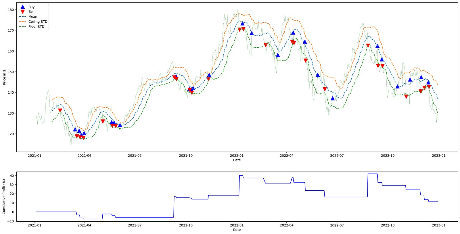

This block begins by generating the trading signals that drive the rest of the pipeline: mean_reversion_signals(aapl_ts_df) consumes the time-series dataframe for AAPL and produces a signals structure indexed by time. That signals object contains the rolling mean and rolling standard deviation used by the strategy, and it also encodes the trade intent (e.g., long/flat/short or entry/exit markers) derived from comparing price to those statistics. We call this first so we have both the statistical thresholds and the discrete trading signals available for downstream profit calculation and visualization.

Next, calculate_profit is invoked with those signals together with the Adjusted Close price series. Its role is to translate the abstract signals into realized P&L: it aligns signals to price timestamps, converts position changes into trades, computes per-period and cumulative returns based on the executed prices, and outputs a returns series that quantifies the strategy’s monetary or percentage performance over time. This step is crucial for quant trading because it converts strategy logic into measurable outcomes that can be tested and compared.

The code then calls plot_strategy with the price series, signals, and returns and captures the returned main axis. plot_strategy draws the primary price chart and typically overlays markers for entries/exits and may plot the cumulative returns on a secondary axis; returning the main axis lets us continue augmenting the price plot. The underscore (_) captures a secondary return value that this snippet does not use, which is often the secondary axis used for returns or volume.

After the base plot is created, the script builds a small collection of series-to-plot: the rolling mean, and the mean shifted up and down by one standard deviation (labelled “Ceiling STD” and “Floor STD”). These represent the statistical band around the expected value — the band width (±std) measures recent volatility and defines the threshold region for mean-reversion decisions. Plotting these lines over the price trace makes it visually apparent when the price deviates far enough from the mean to trigger a reversion trade according to the strategy rules.

The for-loop iterates each (series, label) pair and draws them on the main price axis as dashed lines, using the signals’ index to ensure time alignment with the price. The dashed linestyle visually distinguishes these threshold lines from the price and trade markers. Finally, the call to main_ax.legend places a legend on the upper-left of the plot to associate labels with each plotted series, and plt.show renders the combined visualization. Together these steps produce a single view that ties raw prices, the strategy’s statistical thresholds, the executed signals, and the resulting returns into a coherent diagnostic chart for evaluating the mean-reversion strategy’s behavior.

A 10% on-paper return is respectable, though in practice you might have achieved a similar result by holding a broad S&P 500 index.

In future articles we will examine more advanced mean-reversion approaches, principally pair trading and statistical arbitrage. We will also cover strategy performance metrics (for example, the Sharpe ratio) to explain why a strategy that matches the S&P 500 in raw return can still be considered weak.

Conclusion

We examined simple momentum and mean-reversion trading strategies and analyzed them using Python. Momentum strategies seek to exploit trending behavior to forecast future price movements, while mean-reversion strategies are based on the idea that prices or returns tend to revert toward a long-term average after extreme moves.

In real portfolio trading, no single strategy guarantees success — despite what some online “finfluencers” might claim.

Use the button below to download the source code: