

Building the GPT architecture core
Chapter 7: Implementing GPT configuration, tensor flow, and the modular decoder block from scratch in PyTorch

GPT configuration as the model contract
A GPT model begins with a configuration object that fixes the architectural shape before any weights are learned. That distinction matters. The configuration specifies the size of the vocabulary, the maximum context length, the width of the internal representations, the number of attention heads, the number of stacked blocks, the dropout rate, and whether attention projections include bias terms. These values do not change during training; they define the container in which trainable weights will live.
📘 Buy the Entire Book – Available on Amazon Worldwide (If you are paid subscriber, use the url at the end of this article to download the book for free!)
You can now purchase the complete book directly from Amazon in your country:
GPT_CONFIG_124M = {
    "vocab_size": 50257,
    "context_length": 1024,
    "emb_dim": 768,
    "n_heads": 12,
    "n_layers": 12,
    "drop_rate": 0.1,
    "qkv_bias": False
}
The vocabulary size determines the dimensionality of the final prediction space. The context length sets the longest token sequence the model can process at once. The embedding dimension controls the width of token and position vectors as they move through the network. The head count and layer count determine how much attention computation is distributed across each block and how many times the block is repeated. Dropout introduces stochastic regularization, and the attention bias flag governs whether the query, key, and value projections use bias parameters. Together, these fields describe the model contract that every submodule must obey.
Parameters are the trainable weights inside that contract. Embedding tables, projection matrices, normalization scales, and feed-forward layers all contribute parameters. By contrast, the configuration values are fixed design choices. Keeping that separation clear makes the later implementation easier to read, because each module can be built from the same shared specification.
A dummy GPT stack to preview tensor flow
Before implementing the real transformer internals, it is useful to sketch the full route that data will take through the model. The dummy GPT class below has the same outer structure as the finished network. It starts with token embeddings and positional embeddings, applies dropout, passes the sequence through a stack of placeholder transformer blocks, normalizes the result, and finally maps each hidden vector to vocabulary-sized logits.
class DummyGPTModel(nn.Module):
    def __init__(self, cfg):
        super().__init__()
        self.tok_emb = nn.Embedding(cfg["vocab_size"], cfg["emb_dim"])
        self.pos_emb = nn.Embedding(cfg["context_length"], cfg["emb_dim"])
        self.drop_emb = nn.Dropout(cfg["drop_rate"])
        self.trf_blocks = nn.Sequential(
            *[DummyTransformerBlock(cfg)
              for _ in range(cfg["n_layers"])]
        )
        self.final_norm = DummyLayerNorm(cfg["emb_dim"])
        self.out_head = nn.Linear(
            cfg["emb_dim"], cfg["vocab_size"], bias=False
        )

    def forward(self, in_idx):
        batch_size, seq_len = in_idx.shape
        tok_embeds = self.tok_emb(in_idx)
        pos_embeds = self.pos_emb(
            torch.arange(seq_len, device=in_idx.device)
        )
        x = tok_embeds + pos_embeds
        x = self.drop_emb(x)
        x = self.trf_blocks(x)
        x = self.final_norm(x)
        logits = self.out_head(x)
        return logits

class DummyTransformerBlock(nn.Module):
    def __init__(self, cfg):
        super().__init__()

    def forward(self, x):
        return x

class DummyLayerNorm(nn.Module):
    def __init__(self, normalized_shape, eps=1e-5):
        super().__init__()

    def forward(self, x):
        return x
This skeleton already reveals the full tensor path. The input is a batch of token IDs with shape [batch_size, seq_len]. Token embedding converts each ID into a dense vector, producing [batch_size, seq_len, emb_dim]. Positional embedding generates one learned position vector per time step, and the two are added elementwise so that each token representation carries both identity and order information. After that, dropout preserves the same shape while randomly masking activations during training. The placeholder transformer stack accepts and returns the same three-dimensional tensor, which is exactly what the real blocks will do once attention and feed-forward logic are inserted. The final normalization prepares the hidden states for the output head, and the linear projection produces logits with shape [batch_size, seq_len, vocab_size].
Although the dummy block and dummy normalization do nothing numerically, they are still valuable. They preserve the interface of the eventual GPT implementation, which means the rest of the model can be developed without changing the outer structure. That makes the section a structural preview rather than an approximation of language modeling behavior.
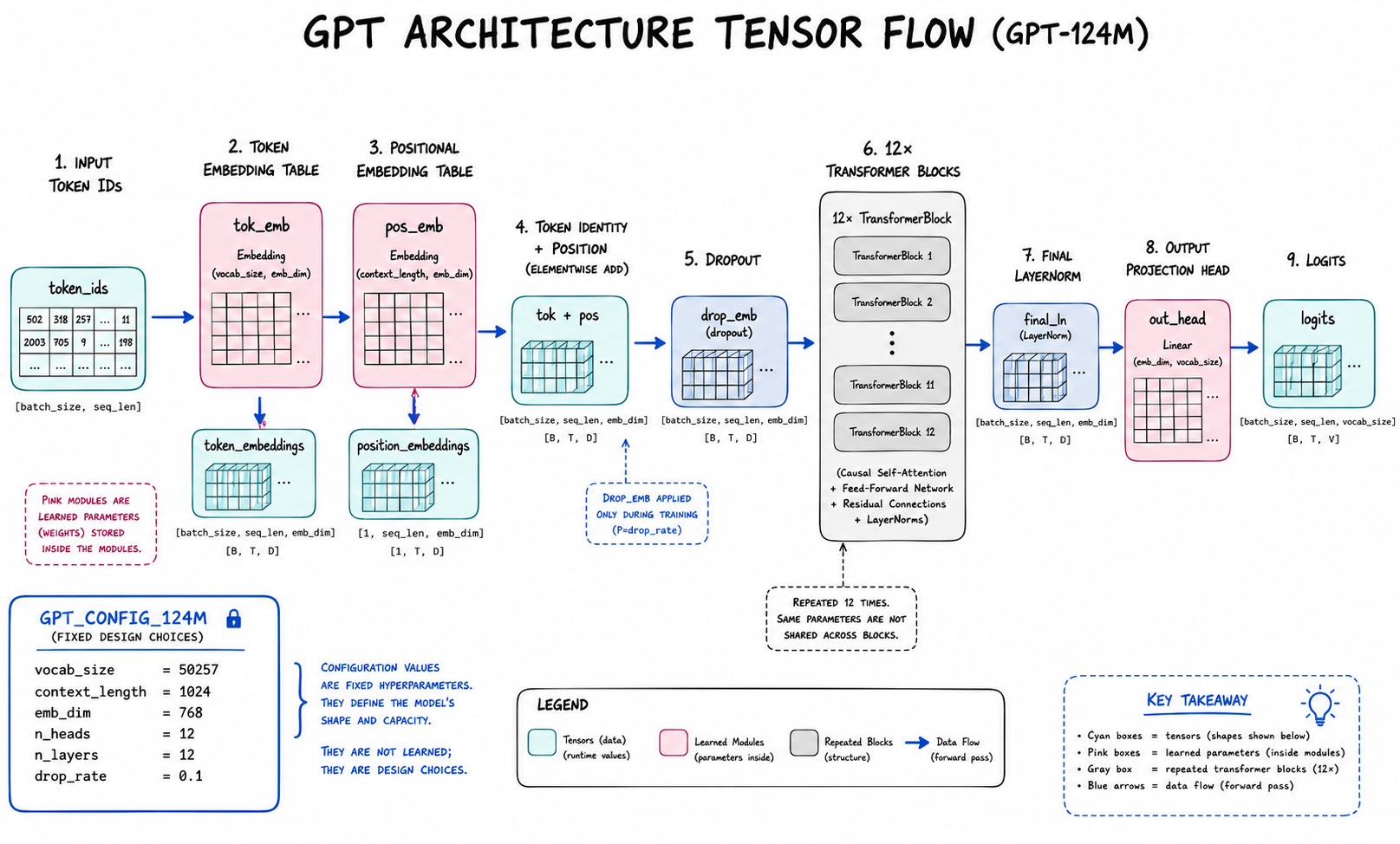
Figure 7.1. The GPT model keeps a stable tensor path: token IDs become token-plus-position embeddings, pass through repeated transformer blocks, and become vocabulary-sized logits.
Tokenizing a toy batch and running the preview model
To make the shape flow concrete, start with two short strings and convert them into a batched tensor of token IDs using the GPT-2 tokenizer. The resulting batch is small enough to inspect directly, yet it already matches the input form expected by the model.
import tiktoken

tokenizer = tiktoken.get_encoding("gpt2")
batch = []
txt1 = "Every effort moves you"
txt2 = "Every day holds a"

batch.append(torch.tensor(tokenizer.encode(txt1)))
batch.append(torch.tensor(tokenizer.encode(txt2)))
batch = torch.stack(batch, dim=0)
print(batch)
The stacked tensor contains token IDs for two sequences. Because the sequences are short, the printed tensor is easy to inspect, but the same batching pattern scales to long sequences as long as they fit inside the configured context length. When that batch is passed into the dummy model, the model returns one vocabulary-sized score vector per token position.
torch.manual_seed(123)
model = DummyGPTModel(GPT_CONFIG_124M)
logits = model(batch)
print("Output shape:", logits.shape)
print(logits)
The output shape confirms the model interface: batch dimension first, sequence length second, vocabulary dimension last. The actual values in the tensor are not meant to be interpreted as meaningful predictions yet, because the central transformer machinery is still a stub. What matters here is that the complete GPT pipeline is already visible. The configuration sets the dimensions, the embeddings convert token IDs into vectors, the placeholder stack preserves the sequence shape, and the output head maps each position back to the vocabulary. In the next sections, the dummy pieces will be replaced by real normalization, activation, attention, and residual logic.
Why normalize token embeddings at all
Deep networks can become difficult to optimize when internal activations drift too far from a well-behaved range. In a GPT-style model, that issue is especially visible once token representations pass through many stacked sublayers. Layer normalization addresses this by keeping each token’s hidden state on a controlled scale before the next computation sees it. The key detail is that GPT normalizes each token independently across its embedding features, not across the batch. That choice makes the method insensitive to batch size and well suited to autoregressive models that process variable-sized batches during training and generation.
This normalization step does not remove information the model needs to learn. Instead, it provides a stable operating point. Once the activations are standardized, later layers can focus on transforming meaning rather than constantly compensating for wildly changing magnitudes. That stability becomes more important as the network grows deeper, where poorly scaled activations can amplify optimization problems and make gradients harder to use effectively.
A worked normalization example on a small activation vector
Suppose a token is represented by a short activation vector. For one example, we can compute the mean and variance across the last dimension and use those statistics to center and scale the vector. The manual normalization rule is
out\_norm=out−μσ2
where μ is the mean of the features in the token vector and σ2 is the corresponding variance. After subtracting the mean and dividing by the standard deviation, the result has zero mean and unit variance along that feature axis.
The final LayerNorm module adds a small stability term to the denominator:
x^=x−μσ2+ϵ
That ϵ prevents division by zero and softens numerical issues when the variance is extremely small. In practice, this matters even when the tensor values are ordinary, because deep models run through many repeated floating-point operations.
A quick toy example makes the mechanics concrete. Imagine a tensor with shape [batch,features], where each row is one token representation. We compute the statistics row by row, normalize each row independently, and then check that the transformed rows are close to zero mean and unit variance. The important point is that the computation runs across the last dimension, so each token is normalized from its own features rather than from other examples in the batch.
Implementing LayerNorm in PyTorch
The reusable module is compact, but each line is doing something essential.
class LayerNorm(nn.Module):
    def __init__(self, emb_dim):
        super().__init__()
        self.eps = 1e-5
        self.scale = nn.Parameter(torch.ones(emb_dim))
        self.shift = nn.Parameter(torch.zeros(emb_dim))

    def forward(self, x):
        mean = x.mean(dim=-1, keepdim=True)
        var = x.var(dim=-1, keepdim=True, unbiased=False)
        norm_x = (x - mean) / torch.sqrt(var + self.eps)
        return self.scale * norm_x + self.shift
The reduction over dim=-1 tells PyTorch to compute statistics along the embedding axis. With GPT tensors, that is the last dimension of a shape such as [batch, num_tokens, emb_dim]. The keepdim=True argument preserves the rank of the tensor, which makes broadcasting work cleanly when subtracting the mean and dividing by the standard deviation.
The call to var(..., unbiased=False) is deliberate. It uses the population-style variance estimate rather than Bessel-corrected sample variance. That choice matches the implementation used in GPT-style models and keeps the behavior aligned with the weights you will later load or reproduce. The epsilon term is added inside the square root, exactly as in the mathematical definition above, so the code and the derivation stay synchronized.
The learnable scale and shift parameters restore flexibility after normalization. Standardization alone would force every token feature toward the same distribution, but the model still needs the ability to reweight or translate those normalized values when that helps the task. LayerNorm therefore standardizes first and then applies a trainable affine transform.
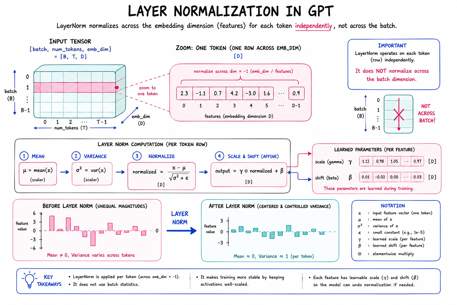
Figure 7.2. LayerNorm normalizes each token independently across its embedding features, then restores flexibility with learned scale and shift parameters.
Checking the output statistics and contrasting with batch normalization
A verification pass should show that the module is doing what the derivation promises. Using a small activation tensor, you can feed the same values through the custom module and then inspect the statistics along the last dimension. The means should be very close to zero, and the variances should be very close to one, up to floating-point error and the small epsilon term.
That behavior differs from batch normalization in an important way. Batch normalization computes statistics across the batch dimension, so its output depends on how many examples happen to be in the mini-batch. Layer normalization does not have that dependency. It normalizes each token independently, which is a better fit for transformer hidden states and for the variable batch sizes commonly used in language modeling. With this module in place, the next step is to place it where the model can use it repeatedly inside each transformer sublayer.
GELU as the transformer’s smooth nonlinearity
A transformer block needs more than attention. After attention mixes information across tokens, each token still needs a private transformation that can reshape its feature vector before the next block sees it. In GPT-style models, that transformation is usually a two-layer feed-forward network with a GELU nonlinearity in the middle.
GELU stands for Gaussian error linear unit. Its exact definition is
where $\Phi(x)$ is the cumulative distribution function of the standard normal distribution. This makes GELU smooth, which is one reason it works well inside deep transformer stacks. Instead of cutting off negative values abruptly, it lets them pass through in a graded way. That softness often leads to smoother optimization than a hard-threshold activation.
A familiar baseline is ReLU, which returns zero for negative inputs and the input itself for positive inputs. GELU behaves differently on the negative side: small negative values are suppressed, but not all at once. That matters in a feed-forward block because the network is not merely filtering features; it is learning a nuanced token-wise transformation. For GPT-style models, the usual implementation uses a fast approximation:
This approximation is accurate enough for practical use and cheaper to evaluate than the exact CDF form.
class GELU(nn.Module):
    def __init__(self):
        super().__init__()

    def forward(self, x):
        return 0.5 * x * (1 + torch.tanh(
            torch.sqrt(torch.tensor(2.0 / torch.pi)) *
            (x + 0.044715 * torch.pow(x, 3))
        ))
Visual comparison with ReLU
The easiest way to see the difference is to compare the two activations on the same input range. ReLU produces a sharp corner at zero, while GELU bends smoothly through that region and leaves a small, nonzero response for some negative values. That shape is often a better fit for transformer MLPs, where the model benefits from gradual feature suppression rather than a hard cutoff.
import matplotlib.pyplot as plt

gelu, relu = GELU(), nn.ReLU()

x = torch.linspace(-3, 3, 100)     #1
y_gelu, y_relu = gelu(x), relu(x)
plt.figure(figsize=(8, 3))
for i, (y, label) in enumerate(zip([y_gelu, y_relu], ["GELU", "ReLU"]), 1):
    plt.subplot(1, 2, i)
    plt.plot(x, y)
    plt.title(f"{label} activation function")
    plt.xlabel("x")
    plt.ylabel(f"{label}(x)")
    plt.grid(True)
plt.tight_layout()
plt.show()
The point of the plot is not that one curve is universally superior. It is that transformer feed-forward layers benefit from a smoother response profile, especially when the network is deep and the activation must cooperate with normalization and residual paths.
Building the position-wise feed-forward module
The feed-forward sublayer is position-wise, which means it processes each token representation independently of the others. Attention has already handled interaction across positions. This module now acts on the feature dimension of each token vector, expanding it into a larger hidden space, applying GELU, and then projecting it back to the model width.
The hidden expansion is a standard design choice in GPT-style architectures. If the embedding dimension is $d{\text{model}}$, the inner layer is typically set to $4d{\text{model}}$. That fourfold expansion gives the MLP room to build richer intermediate features before compressing them back to the original embedding size. The output width must match the input width so the sublayer can fit into the surrounding transformer block without changing tensor layout.
class FeedForward(nn.Module):
    def __init__(self, cfg):
        super().__init__()
        self.layers = nn.Sequential(
            nn.Linear(cfg["emb_dim"], 4 * cfg["emb_dim"]),
            GELU(),
            nn.Linear(4 * cfg["emb_dim"], cfg["emb_dim"]),
        )

    def forward(self, x):
        return self.layers(x)
This module is intentionally simple. The first linear layer widens the representation, the activation introduces nonlinearity, and the second linear layer returns the vector to the original embedding size. Because the operation is applied independently to each token position, the sequence length is unchanged. Only the feature representation within each token is transformed.
In practice, this means a tensor shaped like (batch_size, num_tokens, emb_dim) enters the feed-forward network and exits with the same outer dimensions. That interface is exactly what later transformer blocks need. The module can be stacked repeatedly because every block receives and returns the same embedding width.
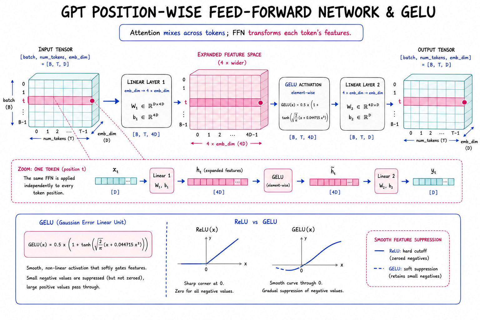
Figure 7.3. The position-wise feed-forward network expands each token from `emb_dim` to `4 × emb_dim`, applies GELU, and projects it back without changing the sequence length.
Checking the tensor interface
A quick shape test is enough to confirm that the submodule behaves as intended. The test below uses the chapter’s configuration object, which already defines the embedding dimension for the model.
ffn = FeedForward(GPT_CONFIG_124M)
x = torch.rand(2, 3, 768)          #1
out = ffn(x)
print(out.shape)
If the implementation is correct, the output shape matches the input shape. That result is not cosmetic; it is the structural requirement that makes the feed-forward network usable inside a transformer block. The block can then combine attention output, normalization, and this MLP sublayer while preserving the same token and embedding interfaces throughout the stack.
Residual connections as an extra path
A residual connection gives a layer two ways to carry information forward. The layer can still learn a transformation of its input, but it can also preserve the original signal by adding that input back to the transformed output. In practice, this means the network does not have to decide between “replace the representation” and “keep the representation.” It can do both, with the shortcut carrying the earlier activation around the main transformation.
That simple elementwise add becomes especially useful in deep networks. When several layers are stacked, each layer only needs to learn the part that changes the representation, rather than rebuilding the entire signal from scratch. For transformer blocks, this idea fits naturally: the block computes an update, then adds that update to the input of the block. The block output remains close to the original representation when needed, while still allowing meaningful transformation when the data demands it.
Why deep stacks become hard to optimize
Without shortcut paths, gradients must pass through every layer in sequence during backpropagation. As depth increases, those gradients can shrink or become poorly scaled before they reach the earliest layers. The result is the familiar vanishing-gradient problem: later layers may still learn, but the layers near the input receive such weak learning signals that training becomes slow or unstable.
Residual paths help because they create a more direct route for both activations and gradients. During the forward pass, the model can preserve useful information instead of repeatedly compressing it through transformations. During the backward pass, the shortcut gives the optimization process a path that is less dependent on the exact behavior of every intermediate transformation. This does not eliminate all training difficulty, but it makes very deep stacks much more practical.
A minimal PyTorch experiment
The following toy network is intentionally small and shape-matched so that the residual add is always valid when the shortcut is enabled. It is not the final GPT block; it is only a clean way to observe what changes when the skip path is present.
class ExampleDeepNeuralNetwork(nn.Module):
    def __init__(self, layer_sizes, use_shortcut):
        super().__init__()
        self.use_shortcut = use_shortcut
        self.layers = nn.ModuleList([
            nn.Sequential(nn.Linear(layer_sizes[0], layer_sizes[1]),
                          GELU()),
            nn.Sequential(nn.Linear(layer_sizes[1], layer_sizes[2]),
                          GELU()),
            nn.Sequential(nn.Linear(layer_sizes[2], layer_sizes[3]),
                          GELU()),
            nn.Sequential(nn.Linear(layer_sizes[3], layer_sizes[4]),
                          GELU()),
            nn.Sequential(nn.Linear(layer_sizes[4], layer_sizes[5]),
                          GELU())
        ])

    def forward(self, x):
        for layer in self.layers:
            layer_output = layer(x)
            if self.use_shortcut and x.shape == layer_output.shape:
                x = x + layer_output
            else:
                x = layer_output
        return x
The key detail is the shape check. Elementwise addition only makes sense when the two tensors have identical shapes, so the shortcut is applied only when the input and the layer output can be added safely. That condition is not a theoretical detail; it is the implementation rule that makes residual connections well-defined.
To compare gradient flow, we can run the same input through a plain stack and through the same stack with shortcuts, then print the mean absolute gradient for every weight tensor after backpropagation.
def print_gradients(model, x):
    output = model(x)
    target = torch.tensor([[0.]])

    loss = nn.MSELoss()
    loss = loss(output, target)

    loss.backward()

    for name, param in model.named_parameters():
        if 'weight' in name:
            print(f"{name} has gradient mean of {param.grad.abs().mean().item()}")
This experiment uses a fixed target and a simple mean-squared error loss so that the only thing we are comparing is how gradients move through depth. The printed values are not a benchmark and they are not a proof. They are a diagnostic view of gradient flow in one concrete example.
Reading the gradient results
In the plain network, gradient magnitudes often become smaller as they reach earlier layers. That is the practical sign of a deep stack that is harder to optimize: the layers farthest from the loss receive weaker updates. With residual paths enabled, the gradient means tend to stay more usable across the stack, which tells you that the learning signal is propagating more effectively.
The important lesson is qualitative rather than numerical. You should read the output as evidence that shortcut connections improve trainability by making gradients less fragile over depth. This is why residuals are not just an architectural convenience. They are one of the mechanisms that allow deep models to be trained at all.
Why GPT blocks rely on this idea
GPT-style transformer blocks repeat the same pattern many times, and each repetition depends on residual paths to keep optimization stable. The attention sublayer and the feed-forward sublayer will each be wrapped in this kind of skip structure so that every block can refine the representation without destroying it. Residual connections are therefore part of the basic grammar of the GPT architecture, not an optional embellishment.
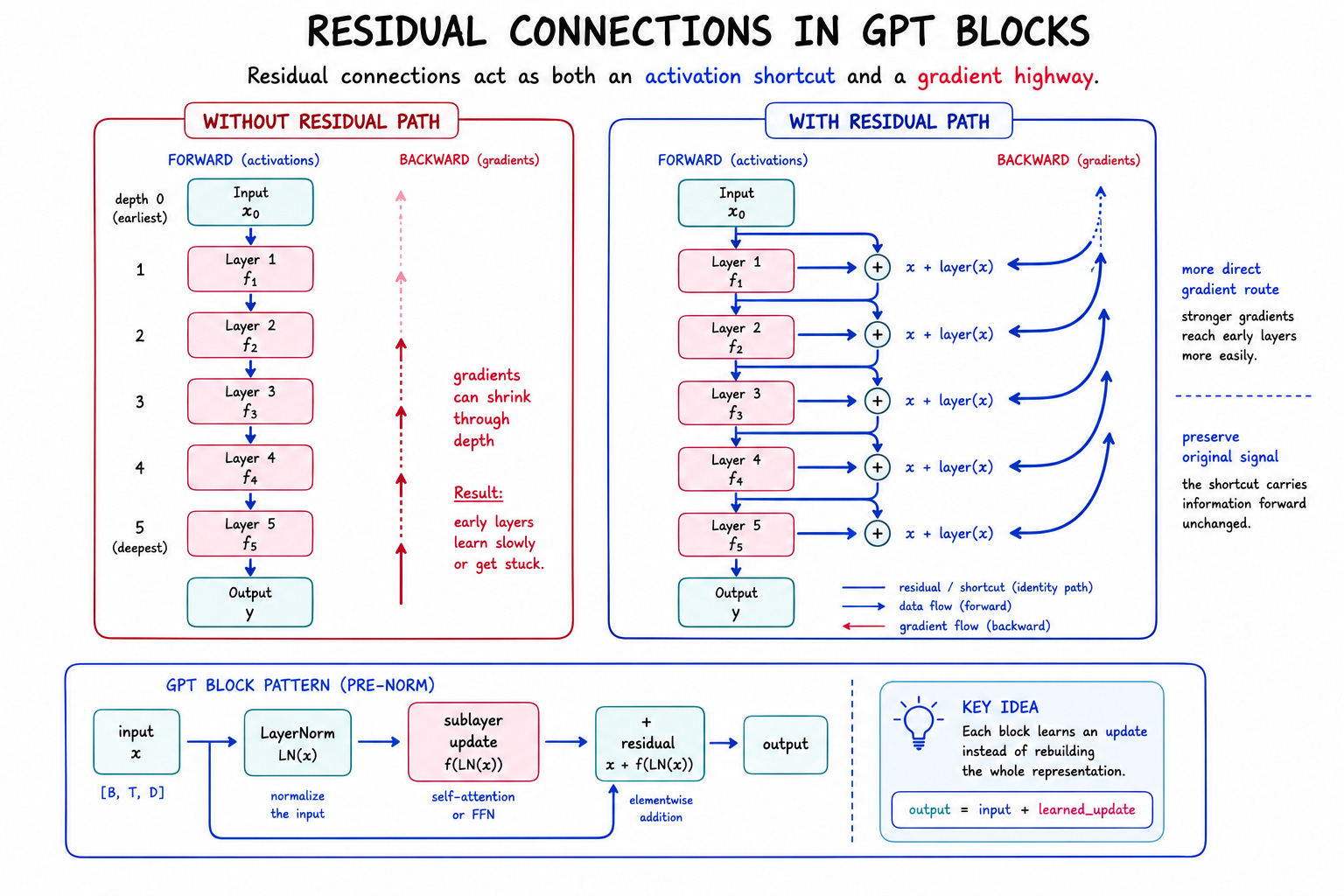
Figure 7.4. Residual connections let each GPT block add a learned update while preserving a direct path for activations and gradients.
Use the url below to download the enitre book as pdf: