Chapter 3: Going on a random walk

A fundamental concept in time series analysis, particularly relevant in financial markets, is the random walk process.

Understanding random walks is crucial because many real-world series, including stock prices, often exhibit this behavior, making them challenging to forecast beyond very short horizons.

Link To Download Source Code at end!

Defining a Random Walk

Conceptually, a random walk is a time series where the current value is equal to the previous value plus a random shock. Imagine a drunkard stumbling through a field: their next position is their current position plus a random step in some direction. This “random step” is the key.

Formally, a random walk process, denoted as Yt, can be defined by the equation:

Yt = Yt − 1 + ϵt

Here: * Yt represents the value of the series at time t. * Yt − 1 represents the value of the series at the previous time step, t − 1. * ϵt (epsilon) represents a white noise error term at time t.

The ϵt term is what makes the walk “random.” It signifies an unpredictable, random fluctuation. For a series to be considered a true random walk, the ϵt term must adhere to the properties of white noise.

Understanding White Noise

White noise is a critical concept in time series. It’s a sequence of random variables that are independent and identically distributed (i.i.d.) with a mean of zero and a constant variance. In simpler terms, for a white noise series: * Mean is zero: On average, the random shocks don’t push the series consistently up or down. * Constant variance: The magnitude of the random shocks doesn’t systematically increase or decrease over time. * No autocorrelation: The current shock ϵt is not correlated with any past shock ϵt − k (where k ≠ 0). This is the most important property for time series analysis: past errors provide no information about future errors.

For a random walk, each new step is entirely independent of the previous steps, influenced only by the current random shock. This means that the best prediction for the next value is simply the current value, as past movements offer no predictive power for the direction or magnitude of the next random step.

Simulating a Simple Random Walk

To solidify our understanding, let’s simulate a basic random walk using Python. We’ll start with a given initial value and then add random steps (our white noise) iteratively.

First, we need to import the necessary libraries: numpy for numerical operations (especially generating random numbers) and matplotlib.pyplot for plotting.

import numpy as np
import matplotlib.pyplot as plt
# Set a random seed for reproducibility
np.random.seed(42)

Here, np.random.seed(42) ensures that if you run this code multiple times, you’ll get the exact same “random” sequence, which is very helpful for debugging and ensuring consistent examples.

Next, we define the starting point for our random walk and how many steps it will take.

# Define the starting point and number of steps
start_value = 100
num_steps = 250

We’ve set our initial value to 100 and decided to simulate 250 time steps.

Now, we generate the random shocks (our white noise) and then compute the random walk by cumulatively summing these shocks from the start_value.

# Generate random steps (white noise)
# These steps are drawn from a normal distribution with mean 0 and standard deviation 1
random_steps = np.random.normal(loc=0, scale=1, size=num_steps)
# Initialize the random walk array with the start value
random_walk = np.zeros(num_steps)
random_walk[0] = start_value
# Compute the random walk by cumulatively adding the steps
for i in range(1, num_steps):
    random_walk[i] = random_walk[i-1] + random_steps[i]

In this block: * np.random.normal(loc=0, scale=1, size=num_steps) creates an array of num_steps random numbers. loc=0 means the average step size is zero, and scale=1 means the typical deviation of a step is 1 unit. This effectively simulates our ϵt white noise. * We initialize random_walk with thestart_value. * The for loop then implements the core random walk equation: Y_t = Y_{t-1} + epsilon_t. Each new value is the previous value plus a new random step.

Finally, let’s visualize our simulated random walk.

# Plot the simulated random walk
plt.figure(figsize=(10, 6))
plt.plot(random_walk, label='Simulated Random Walk')
plt.title('Simulated Random Walk Process')
plt.xlabel('Time Step')
plt.ylabel('Value')
plt.grid(True)
plt.legend()
plt.show()

This code plots the random_walk array over time. When you observe this plot, you’ll notice key visual characteristics: * No clear mean reversion: The series doesn’t tend to return to a particular average value. It wanders without a central tendency. * Persistent trends: While random, the series might appear to trend up or down for periods, but these trends are not deterministic; they are just accumulated random steps. * Unpredictable fluctuations: It’s hard to predict the next value based on previous patterns. Each step seems to be a new, independent shock.

The Importance of Stationarity

One of the most critical concepts in time series analysis is stationarity. Many powerful time series models, such as ARIMA models, assume that the underlying data generating process is stationary.

A time series is considered stationary if its statistical properties — like its mean, variance, and autocorrelation structure — do not change over time. In essence, a stationary series looks roughly the same at any point in time, regardless of when you observe it.

Why is stationarity desirable? 1. Predictability: If the statistical properties of a series are constant over time, we can use past data to make reliable forecasts about future values. If the mean or variance is constantly changing, any model trained on past data might not be relevant for future predictions. 2. Model Simplicity: Many econometric and statistical models are built upon the assumption of stationarity. Non-stationary series often require complex modeling or transformations before standard techniques can be applied. 3. Inference: Statistical inference (e.g., hypothesis testing, confidence intervals) is more straightforward and reliable with stationary data.

A random walk, by its very definition, is a non-stationary process. Its mean is not constant (it wanders), and its variance increases over time (the longer the walk, the further it can deviate from its starting point). This non-stationarity is a significant challenge for forecasting.

Differencing: Achieving Stationarity

Since many models require stationarity, how do we handle non-stationary series like random walks? One common and effective technique is differencing.

Differencing involves computing the difference between consecutive observations in a time series. The goal is to remove trends, seasonality, or other non-stationary components, thereby making the series stationary.

For a simple first-order differencing, we calculate: ΔYt = Yt − Yt − 1

Let’s consider our random walk equation again: Yt = Yt − 1 + ϵt

If we apply first-order differencing to this random walk, we get: Yt − Yt − 1 = (Yt − 1+ϵt) − Yt − 1 Yt − Yt − 1 = ϵt

This result is profound: differencing a random walk yields a white noise series! Since white noise is by definition stationary (constant mean of zero, constant variance, no autocorrelation), differencing successfully transforms a non-stationary random walk into a stationary series.

Let’s apply differencing to our simulated random walk and observe the result.

# Calculate the first-order difference of the simulated random walk
differenced_random_walk = np.diff(random_walk)
# Plot the differenced random walk
plt.figure(figsize=(10, 6))
plt.plot(differenced_random_walk, label='Differenced Random Walk (White Noise)')
plt.title('Differenced Simulated Random Walk')
plt.xlabel('Time Step')
plt.ylabel('Change in Value')
plt.grid(True)
plt.axhline(0, color='red', linestyle='--', linewidth=0.8, label='Mean = 0') # Add a line at y=0
plt.legend()
plt.show()

The np.diff() function calculates the difference between consecutive elements in an array. When you plot differenced_random_walk, you’ll see a series that fluctuates randomly around zero, with no apparent trend or changing variance. This visually confirms that we’ve transformed the non-stationary random walk into a stationary white noise series.

The Autocorrelation Function (ACF)

Beyond visual inspection, a powerful statistical tool for identifying the properties of a time series, including its stationarity and the presence of random walk behavior, is the Autocorrelation Function (ACF).

The ACF measures the correlation between a time series and its lagged values. For example: * ACF at lag 1: Correlation between Yt and Yt − 1. * ACF at lag 2: Correlation between Yt and Yt − 2. * And so on.

By plotting the ACF values for various lags, we get an autocorrelation plot (often called a correlogram). * For a stationary series, the ACF typically drops off quickly to zero. This indicates that past values have little to no linear relationship with current values beyond a few lags. * For a random walk (non-stationary series), the ACF plot shows a very distinct pattern: it decays very slowly. This slow decay indicates strong, persistent correlation between current values and past values, which is characteristic of a non-stationary series where past values heavily influence current values without mean reversion. * For white noise, the ACF values are close to zero for all lags (except lag 0, which is always 1). This confirms that there is no linear relationship between a value and its past values.

Understanding the ACF is crucial for identifying the underlying process of a time series and for selecting appropriate forecasting models.

Random Walks in the Real World: GOOGL Stock Prices

One of the most prominent real-world examples of time series that often behave like random walks are financial asset prices, particularly stock prices. Let’s consider the closing price of Google stock (GOOGL).

The reason stock prices often resemble random walks is tied to the Efficient Market Hypothesis (EMH). In its strong form, EMH suggests that all available information is immediately and fully reflected in asset prices. This implies that future price movements are unpredictable because any predictable patterns would have already been exploited by traders, driving the price to reflect that information instantly. Therefore, the only thing that can move the price is new, unpredictable information, which effectively acts like the “random shock” (ϵt) in our random walk equation.

Let’s load and plot some historical GOOGL stock data to see this in action. We’ll use pandas for data handling and matplotlib for plotting.

import pandas as pd
import matplotlib.pyplot as plt
# Load the GOOGL dataset (assuming it's in a CSV file named 'GOOGL.csv'
# in the same directory, with a 'Date' column and a 'Close' column)
# For demonstration, we'll create a dummy DataFrame if the file isn't present.
try:
    googl_df = pd.read_csv('GOOGL.csv', parse_dates=['Date'], index_col='Date')
except FileNotFoundError:
    print("GOOGL.csv not found. Creating a dummy dataset for demonstration.")
    # Create a dummy random walk-like dataset for demonstration purposes
    np.random.seed(43) # Different seed for dummy data
    dummy_start_value = 1500
    dummy_num_steps = 500
    dummy_random_steps = np.random.normal(loc=0.5, scale=5, size=dummy_num_steps) # A slight positive drift
    dummy_random_walk_data = np.cumsum(np.insert(dummy_random_steps, 0, dummy_start_value))[:-1] # Correct length
    dummy_dates = pd.date_range(start='2020-01-01', periods=dummy_num_steps, freq='B') # Business days
    googl_df = pd.DataFrame({'Close': dummy_random_walk_data}, index=dummy_dates)
# Display the first few rows of the DataFrame
print("GOOGL Data Head:")
print(googl_df.head())
# Display basic information about the DataFrame
print("\nGOOGL Data Info:")
googl_df.info()

This code snippet attempts to load a GOOGL.csv file. If the file is not found (which is likely for a generic example), it creates a dummy DataFrame that simulates random walk behavior, ensuring the code runs and demonstrates the plotting. The parse_dates=['Date'] and index_col='Date' arguments are crucial for treating the ‘Date’ column as a proper datetime index, which is standard practice for time series data.

Now, let’s plot the closing prices of GOOGL.

# Plot the GOOGL closing prices
plt.figure(figsize=(12, 7))
plt.plot(googl_df['Close'], label='GOOGL Closing Price')
plt.title('GOOGL Stock Closing Prices (Example of a Random Walk)')
plt.xlabel('Date')
plt.ylabel('Price (USD)')
plt.grid(True)
plt.legend()
plt.tight_layout()
plt.show()

When you examine this plot, you’ll see characteristics very similar to our simulated random walk: * No clear mean reversion: The price doesn’t consistently return to a fixed average. * Apparent trends: There might be periods of sustained upward or downward movement, but these are generally not deterministic and can reverse unpredictably. * Unpredictability: It’s very difficult to forecast the exact next day’s price movement from the chart alone.

For a series that behaves like a random walk, the most effective “forecast” is often simply the last observed value. This is precisely the naive forecast we discussed in the previous chapter. If today’s GOOGL price is $X, the best forecast for tomorrow’s price, given a random walk assumption, is also $X. This highlights why understanding random walks is so important: it tells us when simple baseline models might be the most appropriate forecasting approach.

The Random Walk Process

Understanding the behavior of time series data is fundamental to effective forecasting. While some series exhibit clear patterns or stationarity, others appear to move unpredictably. Among these, the random walk process stands out as a critical concept, particularly prevalent in financial markets and economic data. A random walk describes a process where the current value is derived from the previous value plus a random shock. This seemingly simple definition has profound implications for how we model and forecast such series.

Defining the Random Walk

At its core, a random walk is a mathematical model for a sequence of random steps. Imagine a person taking steps, where each step’s direction and size are random. The person’s position at any given time is the sum of all previous steps. In time series, this translates to the current observation being the sum of the previous observation and a random, unpredictable change.

The mathematical expression of a random walk process is given by:

y_t = C + y_{t-1} + ε_t

Let’s break down each component of this equation:

• y_t: This represents the value of the time series at the current time point t. It’s what we are trying to model or predict.

• y_{t-1}: This is the value of the time series at the previous time point, t-1. The equation clearly shows a strong dependence on the immediate past value, which is a defining characteristic of a random walk.

• C: This is a constant term, often referred to as the drift. It represents the average step size or the systematic tendency of the series to increase or decrease over time.

• ε_t (epsilon_t): This is the white noise error term or “random shock” at time t. This term is the unpredictable part of the random walk, representing the random fluctuations that occur from one period to the next.

Deconstructing White Noise (ε_t)

The ε_t term is the engine of randomness in a random walk. It’s what makes the series unpredictable in the short term and drives its erratic long-term behavior. To truly understand a random walk, we must understand the properties of white noise.

White noise is a sequence of random variables with the following key properties:

1. Zero Mean: The expected value (average) of ε_t is zero, i.e., E[ε_t] = 0. This means that, on average, the random shocks do not systematically push the series up or down. They are equally likely to be positive or negative.

2. Constant Variance: The variance of ε_t is constant over time, i.e., Var[ε_t] = σ² (sigma squared). This implies that the magnitude of the random shock is consistent and does not grow or shrink over time.

3. No Autocorrelation: The white noise terms are independent of each other. The covariance between ε_t and ε_s is zero for any t ≠ s. This means that a shock at one point in time provides no information about a shock at any other point in time. There are no patterns or memory in the error terms themselves.

Often, for simplicity and analytical convenience, ε_t is assumed to be a realization of a standard normal distribution. This means that ε_t values are drawn from a normal distribution with a mean of 0 and a variance (and thus standard deviation) of 1, denoted as N(0, 1).

Why N(0, 1)? * Symmetry: The normal distribution is symmetric around its mean (0), reinforcing the idea that positive and negative shocks are equally likely. * Mathematical Tractability: It simplifies many statistical analyses and theoretical derivations. * Central Limit Theorem: In many real-world scenarios, random errors or sums of many small, independent random effects tend to converge to a normal distribution.

The choice of N(0, 1) specifically for white noise implies that the random number has an “equal chance of going up or down by a random number” because the distribution is centered at zero. While the standard normal distribution is common, white noise can technically come from any distribution that satisfies the three properties above (zero mean, constant variance, no autocorrelation). However, the implications of using other distributions (e.g., a uniform distribution or a t-distribution) would primarily affect the shape of the distribution of the shocks, potentially leading to more extreme values (fat tails for t-distribution) or bounded values (uniform distribution). For most introductory purposes, the standard normal assumption is sufficient and widely used.

The Role of Drift (C)

The constant C plays a crucial role in determining the long-term behavior of a random walk.

• Pure Random Walk (when C = 0): If C = 0, the equation simplifies to y_t = y_{t-1} + ε_t. In this case, the series has no inherent tendency to increase or decrease. It simply wanders randomly around its starting point. While it can deviate significantly from its initial value, it does so without a systematic direction. Think of a drunkard stumbling around a lamp post – they might wander far, but there’s no overall direction to their movement.

• Random Walk with Drift (when C ≠ 0): If C is a non-zero value, it introduces a systematic trend into the series.

• If C > 0, the series will tend to increase over time, on average, by C units per period, in addition to the random shock.

• If C < 0, the series will tend to decrease over time. The drift term ensures that, in the long run, the series will move predictably in the direction of C, even with the superimposed random fluctuations. Consider the drunkard now walking on a slight incline – they still stumble randomly, but there’s an underlying tendency to move uphill or downhill.

Observed Characteristics and the Equation

The mathematical formulation of a random walk directly explains its observed characteristics:

• Long periods of apparent trend: Even in a pure random walk (C=0), the cumulative effect of the ε_t terms can lead to extended periods where the series appears to trend upwards or downwards. This is purely coincidental, as there’s no underlying systematic trend. With drift (C ≠ 0), these trends become even more pronounced and systematic.

• Sudden changes in direction: Large positive or negative ε_t values can cause the series to abruptly change its direction or significantly accelerate its movement in a particular direction.

• Non-stationarity: A key implication of the random walk equation is that the series is non-stationary. This means its statistical properties (like mean and variance) change over time.

• The mean of a random walk with drift will change over time (it will tend towards C*t).

• The variance of a random walk grows with time (Var[y_t] = t * σ²). This property means that the further out you go in time, the wider the possible range of values for y_t becomes, making long-term forecasting very uncertain.

Numerical Step-by-Step Example

Let’s illustrate how a random walk sequence is generated with a simple numerical example.

Assume: * Initial value y_0 = 100 * Drift C = 1 * A sequence of white noise values ε_t: [0.5, -1.2, 0.8, -0.3, 1.5]

Let’s calculate the first few steps:

• Time t=1: y_1 = C + y_0 + ε_1 y_1 = 1 + 100 + 0.5 = 101.5

• Time t=2: y_2 = C + y_1 + ε_2 y_2 = 1 + 101.5 + (-1.2) = 101.3

• Time t=3: y_3 = C + y_2 + ε_3 y_3 = 1 + 101.3 + 0.8 = 103.1

• Time t=4: y_4 = C + y_3 + ε_4 y_4 = 1 + 103.1 + (-0.3) = 103.8

• Time t=5: y_5 = C + y_4 + ε_5 y_5 = 1 + 103.8 + 1.5 = 106.3

This step-by-step process shows how the series evolves, with each new value building on the previous one, influenced by the constant drift and the random shock.

Simulating Random Walks in Python

To truly grasp the dynamics of a random walk, simulating one is invaluable. We’ll use Python’s numpy library for numerical operations and matplotlib for plotting.

First, let’s import the necessary libraries.

import numpy as np
import matplotlib.pyplot as plt
# Set a random seed for reproducibility
np.random.seed(42)

We import numpy for numerical operations, especially for generating random numbers, and matplotlib.pyplot for plotting. Setting a random seed ensures that our simulations are reproducible; running the code multiple times will yield the same random walk path.

Simulating a Pure Random Walk (C = 0)

A pure random walk has no drift, meaning C = 0. The series simply accumulates random shocks.

# Define parameters for the pure random walk
n_steps = 200  # Number of time steps to simulate
initial_value = 0  # y_0, starting point of the walk
mean_epsilon = 0   # Mean of the white noise
std_epsilon = 1    # Standard deviation of the white noise (for N(0,1))

Here, we define the simulation parameters. n_steps determines the length of our time series. We start initial_value at 0 for simplicity, and define the properties of our white noise (epsilon_t) as a standard normal distribution (mean_epsilon=0, std_epsilon=1).

# Generate white noise (epsilon_t)
# These are the random shocks at each step
epsilon_values = np.random.normal(loc=mean_epsilon, scale=std_epsilon, size=n_steps)

We use np.random.normal to generate n_steps random numbers that follow a normal distribution with the specified mean and standard deviation. These are our epsilon_t values for each time step.

# Initialize the random walk series
pure_rw_series = np.zeros(n_steps + 1) # +1 for y_0
pure_rw_series[0] = initial_value
# Simulate the random walk
for t in range(n_steps):
    # y_t = y_{t-1} + epsilon_t (since C=0)
    pure_rw_series[t+1] = pure_rw_series[t] + epsilon_values[t]

We create an array pure_rw_series to store the values of our random walk, initializing the first element with initial_value. Then, we loop through each time step, applying the random walk formula: the current value is the previous value plus the corresponding random shock.

# Plot the pure random walk
plt.figure(figsize=(12, 6))
plt.plot(pure_rw_series, label='Pure Random Walk (C=0)', color='blue')
plt.title('Simulation of a Pure Random Walk')
plt.xlabel('Time Step')
plt.ylabel('Value')
plt.grid(True)
plt.legend()
plt.show()

Finally, we plot the generated series. You will observe that the path appears to wander without a clear direction, often exhibiting what looks like trends for periods, only to reverse. This visual behavior is a direct consequence of the cumulative random shocks.

Simulating a Random Walk with Drift (C ≠ 0)

Now, let’s introduce a non-zero drift term C to see its effect.

# Define parameters for the random walk with drift
drift_constant = 0.5 # Our constant C

We define drift_constant as our C value. A positive value means the series will tend to increase over time.

# Initialize the random walk with drift series
rw_drift_series = np.zeros(n_steps + 1)
rw_drift_series[0] = initial_value # Start from the same initial value
# Simulate the random walk with drift
for t in range(n_steps):
    # y_t = C + y_{t-1} + epsilon_t
    rw_drift_series[t+1] = drift_constant + rw_drift_series[t] + epsilon_values[t]

Similar to the pure random walk, we initialize the series and loop through the steps. The key difference is the addition of drift_constant in each iteration, systematically pushing the series in one direction. We reuse the same epsilon_values for direct comparison with the pure random walk.

# Plot both random walks for comparison
plt.figure(figsize=(12, 6))
plt.plot(pure_rw_series, label='Pure Random Walk (C=0)', color='blue', alpha=0.7)
plt.plot(rw_drift_series, label=f'Random Walk with Drift (C={drift_constant})', color='red', alpha=0.7)
plt.title('Comparison of Pure Random Walk vs. Random Walk with Drift')
plt.xlabel('Time Step')
plt.ylabel('Value')
plt.grid(True)
plt.legend()
plt.show()

By plotting both series together, the impact of the drift term becomes immediately apparent. The random walk with drift will show a clear upward (or downward, if C were negative) trajectory, even with the random fluctuations superimposed. This illustrates how a constant drift can fundamentally change the long-term behavior of a series.

Practical Applications

The random walk model, especially the concept of a random walk with drift, is widely used in finance to model asset prices, such as stock prices or exchange rates. The Efficient Market Hypothesis in its weak form suggests that stock prices follow a random walk, meaning past price movements cannot be used to predict future movements, as all available information is already reflected in the current price. While real-world financial series are more complex, the random walk serves as a powerful baseline and a crucial concept for understanding non-stationary data. Beyond finance, random walks are used in physics (Brownian motion), biology (population dynamics), and other fields where cumulative random changes occur.

Simulating a Random Walk Process

Building upon the theoretical understanding of random walk processes, this section transitions into their practical simulation and visualization using Python. Simulating these processes is crucial for developing intuition about their behavior, understanding their properties, and preparing for more complex time series modeling tasks.

The Building Block: White Noise

At the heart of a simple random walk is a concept known as white noise. Conceptually, white noise represents a series of purely random, unpredictable shocks or innovations that drive the changes in the random walk process.

Formally, a series of random variables ϵt is considered white noise if it satisfies the following conditions: * Zero Mean: The expected value of each ϵt is zero, i.e., E[ϵt] = 0. This means, on average, the shocks do not systematically push the series up or down. * Constant Variance: The variance of each ϵt is constant and finite, i.e., Var(ϵt) = σ2 < ∞. This implies that the magnitude of the shocks does not change over time. * No Autocorrelation: The covariance between any two different shock terms is zero, i.e., Cov(ϵt,ϵs) = 0 for t ≠ s. This is a critical property, meaning that past shocks provide no information about future shocks; they are independent.

In many practical simulations, especially for pedagogical purposes, white noise is often generated from a standard normal distribution, where ϵt ∼ N(0,1). This means each shock has a mean of 0 and a variance of 1.

The Random Walk as a Cumulative Sum

Recall the mathematical formulation of a simple random walk:

yt = yt − 1 + ϵt

where yt is the value of the random walk at time t, yt − 1 is the value at the previous time step, and ϵt is a white noise term.

Let’s expand this equation step-by-step to see why a random walk is essentially a cumulative sum of white noise. Assume an initial value y0 = 0 for simplicity:

y1 = y0 + ϵ1 = 0 + ϵ1 = ϵ1 y2 = y1 + ϵ2 = (ϵ1) + ϵ2 y3 = y2 + ϵ3 = (ϵ1+ϵ2) + ϵ3

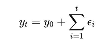
Following this pattern, for any time t, the value of the random walk yt is the sum of all white noise terms up to time t:

$y_t = \sum_{i=1}^{t} \epsilon_i$

This direct relationship to a cumulative sum is fundamental for understanding and simulating random walks.

To illustrate this with a small, concrete example, consider a random walk over 5 steps starting at y0 = 0, with the following generated white noise values: ϵ1 = 0.5 ϵ2 = − 0.2 ϵ3 = 0.8 ϵ4 = 0.1 ϵ5 = − 0.4

The random walk values would be: y0 = 0 (Initial value) y1 = y0 + ϵ1 = 0 + 0.5 = 0.5 y2 = y1 + ϵ2 = 0.5 + (−0.2) = 0.3 y3 = y2 + ϵ3 = 0.3 + 0.8 = 1.1 y4 = y3 + ϵ4 = 1.1 + 0.1 = 1.2 y5 = y4 + ϵ5 = 1.2 + (−0.4) = 0.8

As you can see, each step is simply the previous value plus a new random shock.

Simulating a Basic Random Walk in Python

We will now simulate a basic random walk using Python. Our goal is to create a random walk series that starts at zero and is driven by standard normal white noise.

First, we need to import the necessary libraries: numpy for numerical operations (especially random number generation and cumulative sums) and matplotlib.pyplot for plotting.

import numpy as np
import matplotlib.pyplot as plt
# Set a random seed for reproducibility
# This ensures that every time you run the code, you get the same random numbers,
# making your simulations consistent and verifiable.
np.random.seed(42)

Setting a random seed is a crucial best practice in any simulation. It allows you to reproduce the exact sequence of “random” numbers generated by the computer. Without it, each run of the code would produce a different random walk, making it challenging to debug or compare results. The number 42 is arbitrary; any integer can be used.

Next, we generate the white noise terms, which will serve as the “steps” or “innovations” for our random walk. We’ll simulate 1000 time steps.

# Define the number of steps for our random walk
num_steps = 1000
# Generate 'num_steps' random numbers from a standard normal distribution (mean=0, std=1)
# These represent the 'epsilon_t' (white noise) terms for each time step.
epsilon_steps = np.random.standard_normal(num_steps)
# To ensure our random walk starts at 0 (y_0 = 0), we explicitly set the first 'step' to 0.
# This makes the first value of the cumulative sum also 0, aligning with y_0=0.
epsilon_steps[0] = 0.0
print(f"First 5 epsilon_steps (innovations): {epsilon_steps[:5]}")

The num_steps variable determines the length of our simulated time series. A value of 1000 steps is typically sufficient to observe the characteristic behaviors of a random walk. np.random.standard_normal(num_steps) generates an array of 1000 random numbers drawn from a standard normal distribution. These are our ϵt values. Setting epsilon_steps[0] = 0.0 ensures that when we compute the cumulative sum, the random walk series effectively starts at a value of zero, as its first “change” from an implicit y0 will be zero.

Now, we compute the random walk by applying the cumulative sum to our epsilon_steps.

# Calculate the cumulative sum of the epsilon_steps to generate the random walk series.
# This directly implements y_t = sum(epsilon_i from i=1 to t).
random_walk = np.cumsum(epsilon_steps)
print(f"First 5 random_walk values: {random_walk[:5]}")

The np.cumsum() function is perfectly suited for this task. It takes an array and returns an array where each element is the cumulative sum of the elements up to that position in the input array. For example, [a, b, c] becomes [a, a+b, a+b+c]. Since we set epsilon_steps[0] to 0, random_walk[0] will also be 0, correctly representing our starting point y0.

Finally, we visualize the simulated random walk using matplotlib.

# Create a figure and an axes object for plotting
fig, ax = plt.subplots(figsize=(10, 6))
# Plot the simulated random walk
ax.plot(random_walk, label='Simulated Random Walk')
# Set labels for the x and y axes
ax.set_xlabel('Time Step')
ax.set_ylabel('Value')
# Set the title of the plot
ax.set_title('Simulated Random Walk Process (No Drift, y_0=0)')
# Add a grid for better readability
ax.grid(True)
# Display the legend
ax.legend()
# Adjust plot layout to prevent labels from overlapping
plt.tight_layout()
# Show the plot
plt.show()

The plot will reveal the characteristic behaviors of a random walk: * Non-Stationarity: Unlike stationary series that tend to revert to a mean, random walks can wander significantly from their starting point. * No Mean Reversion: There’s no inherent tendency for the series to return to a central value. * Long-Term Trends: Even without an explicit “drift” term, random walks can exhibit apparent trends (upward or downward) over long periods due to the accumulation of random shocks. These trends are not deterministic but are merely the result of the random process. * Sudden Changes: The series can experience abrupt shifts in direction.

This visual representation is crucial for recognizing random walk behavior in real-world data, such as financial asset prices.

Variations of the Random Walk

The basic random walk simulation demonstrates the core concept. However, random walks can have additional components that influence their behavior.

Random Walk with Drift

A random walk with drift includes a constant term C that systematically pushes the series in one direction (upwards if C > 0, downwards if C < 0). This is represented as:

yt = C + yt − 1 + ϵt

Expanding this, we get:

$y_t = y_0 + C \cdot t + \sum_{i=1}^{t} \epsilon_i$

The C * t term clearly shows the linear trend introduced by the drift.

Let’s simulate a random walk with a positive drift and compare it to our original simulation.

# Define a drift constant
drift = 0.1
# Generate new epsilon_steps for clarity, though you could reuse the previous ones
# For a more direct comparison, we'll reuse the original epsilon_steps and add drift.
# (Ensure epsilon_steps[0] is still 0 if you want y_0=0 for the drift walk too)
# Calculate the random walk with drift
# Each step now includes the constant drift term
drift_random_walk = np.cumsum(epsilon_steps + drift)
# Plot both the original and the drift random walk for comparison
fig, ax = plt.subplots(figsize=(10, 6))
ax.plot(random_walk, label='Simulated Random Walk (No Drift)')
ax.plot(drift_random_walk, label=f'Simulated Random Walk (Drift = {drift})', linestyle='--')
ax.set_xlabel('Time Step')
ax.set_ylabel('Value')
ax.set_title('Simulated Random Walks: No Drift vs. With Drift')
ax.grid(True)
ax.legend()
plt.tight_layout()
plt.show()

You will observe that the random walk with drift tends to move consistently in the direction of the drift over the long term, creating a more pronounced upward or downward trend compared to the no-drift version, which wanders aimlessly. This drift term is particularly relevant in financial modeling, where assets might have an expected positive return over time.

Random Walk with a Non-Zero Initial Value

Another common variation is a random walk that starts at a value other than zero. This simply shifts the entire series up or down by a constant amount.

Here, y0 is the initial value.

# Define a non-zero initial value
initial_value = 50.0
# Calculate the random walk with a non-zero initial value
# We add the initial value to the entire cumulative sum of errors.
initial_value_random_walk = initial_value + np.cumsum(epsilon_steps)
# Plot this new random walk
fig, ax = plt.subplots(figsize=(10, 6))
ax.plot(initial_value_random_walk, label=f'Simulated Random Walk (y_0 = {initial_value})')
ax.set_xlabel('Time Step')
ax.set_ylabel('Value')
ax.set_title(f'Simulated Random Walk Process (Starting at {initial_value})')
ax.grid(True)
ax.legend()
plt.tight_layout()
plt.show()

This simulation will look identical in shape to the original zero-starting random walk, but it will be vertically shifted so that it begins at the specified initial_value. This demonstrates that the starting point primarily affects the level of the series, not its fundamental random walk behavior.

Practical Applications and Implications

Simulating random walks provides critical insights into real-world phenomena:

• Financial Markets: Stock prices, exchange rates, and commodity prices are often modeled as random walks (or variations thereof) in the short term. The Efficient Market Hypothesis suggests that asset prices follow a random walk, meaning future price movements are unpredictable based on past movements. Understanding this helps traders and analysts recognize that apparent patterns in price charts might just be random fluctuations.

• Brownian Motion: In physics, the random movement of particles suspended in a fluid (Brownian motion) is a classic example of a random walk.

• Sensor Readings: Certain types of sensor data, especially in noisy environments, can exhibit random walk characteristics.

• Identifying Non-Stationarity: Random walks are prime examples of non-stationary time series. Their mean and variance are not constant over time (e.g., the variance grows with time, and the “mean” can drift). Recognizing this non-stationarity is a crucial first step in time series analysis, as many traditional forecasting models (like ARIMA) assume stationarity. Often, differencing a random walk (i.e., taking yt − yt − 1 = ϵt) transforms it into a stationary white noise process.

Saving Your Plots

For reports, presentations, or future reference, it’s often useful to save your generated plots to a file. matplotlib makes this straightforward.

# Re-create the plot from the basic random walk simulation for saving
fig, ax = plt.subplots(figsize=(10, 6))
ax.plot(random_walk, label='Simulated Random Walk')
ax.set_xlabel('Time Step')
ax.set_ylabel('Value')
ax.set_title('Simulated Random Walk Process (For Saving)')
ax.grid(True)
ax.legend()
plt.tight_layout()
# Save the figure to a file
# You can specify different formats like .png, .jpg, .pdf, .svg
# 'dpi' (dots per inch) controls the resolution of the saved image.
fig.savefig('random_walk_simulation.png', dpi=300)
print("Plot saved as random_walk_simulation.png")
# Close the plot to free up memory (optional, especially if not showing)
plt.close(fig)

Saving plots ensures that your results are reproducible and easily shareable without needing to rerun the entire simulation.

Identifying a Random Walk

Understanding whether a time series exhibits a random walk behavior is a critical step in time series analysis and forecasting. A random walk process has unique characteristics that dictate the appropriate modeling approach.

Defining a Random Walk Through Its Properties

At its core, a time series is considered a random walk if its first difference is a stationary and uncorrelated process. Let’s break down these crucial components.

Recall from previous sections that a random walk is defined by the equation: Yt = Yt − 1 + ϵt

Where Yt is the value at time t, Yt − 1 is the value at the previous time step, and ϵt is a white noise error term.

If we rearrange this equation, we get: Yt − Yt − 1 = ϵt

The term Yt − Yt − 1 is what we call the first difference of the series Yt. This simple rearrangement reveals the fundamental characteristic: the first difference of a random walk is simply the white noise error term, ϵt.

Since ϵt is by definition a white noise process, it is both stationary and uncorrelated. Therefore, the defining features of a random walk are:

1. Its first difference is stationary.

2. Its first difference is uncorrelated (i.e., it behaves like white noise).

Let’s explore these concepts in more detail.

The First Difference: Capturing Change

The first difference of a time series, denoted as ΔYt or Y′t, is simply the change in the value of the series from one time step to the next. It is calculated as Yt − Yt − 1. This operation is incredibly powerful because it transforms a series of absolute values into a series of changes.

Consider a simple numerical example to illustrate the first difference:

Time (t)Original Series (Yt)First Difference (ΔYt = Yt − Yt − 1)110–21212 − 10 = 231111 − 12 = − 141313 − 11 = 251414 − 13 = 1

Notice that the first difference series starts from the second data point, as the first difference requires a preceding value.

In Python, calculating the first difference is straightforward using the diff() method available for pandas Series or DataFrames. Let’s simulate a simple random walk and observe its first difference.

import numpy as np
import pandas as pd
import matplotlib.pyplot as plt
# Set a seed for reproducibility
np.random.seed(42)
# Generate a synthetic random walk
# Start at 100 and add random steps (white noise)
steps = np.random.normal(loc=0, scale=1, size=100) # White noise errors
random_walk = np.cumsum(steps) + 100 # Cumulative sum of steps starting at 100
# Convert to a pandas Series for easy differencing
rw_series = pd.Series(random_walk)
print("Original Random Walk (first 5 values):\n", rw_series.head())

This code snippet first imports necessary libraries and sets a random seed for consistent results. It then generates a sequence of random steps, representing the white noise errors (ϵt), and cumulatively sums them to create a random walk series. We convert this numpy array into a pandas Series, which provides convenient time series functionalities.

Now, let’s compute its first difference:

# Calculate the first difference
rw_diff = rw_series.diff().dropna() # .dropna() removes the first NaN value
print("\nFirst Difference of Random Walk (first 5 values):\n", rw_diff.head())
print(f"\nOriginal series length: {len(rw_series)}")
print(f"Differenced series length: {len(rw_diff)}")

Here, rw_series.diff() computes the difference between consecutive elements. The first element of the differenced series will be NaN because there is no preceding value to subtract from. We use .dropna() to remove this NaN value, resulting in a differenced series that is one element shorter than the original.

Visualizing both the original random walk and its first difference highlights the transformation:

# Plot the original random walk and its first difference
plt.figure(figsize=(12, 6))
# Plot original random walk
plt.subplot(2, 1, 1) # 2 rows, 1 column, first plot
plt.plot(rw_series)
plt.title('Simulated Random Walk')
plt.xlabel('Time')
plt.ylabel('Value')
plt.grid(True)
# Plot first difference
plt.subplot(2, 1, 2) # 2 rows, 1 column, second plot
plt.plot(rw_diff, color='orange')
plt.title('First Difference of Random Walk')
plt.xlabel('Time')
plt.ylabel('Change in Value')
plt.grid(True)
plt.tight_layout() # Adjust layout to prevent overlapping titles/labels
plt.show()

The top plot shows a typical random walk: it drifts without a clear mean and its variance appears to increase over time. The bottom plot, however, shows the first difference, which fluctuates around zero with a relatively constant variance. This visual difference is a strong hint about the underlying properties we’re about to discuss.

Stationarity: A Stable Baseline

A time series is considered stationary if its statistical properties (mean, variance, and autocorrelation structure) remain constant over time. In simpler terms, a stationary series looks roughly the same regardless of when you observe it.

Random walks are inherently non-stationary. They typically exhibit a trend (even if it’s just a random drift) and their variance tends to increase over time, meaning they spread out more as time progresses. This non-stationarity makes them difficult to model with traditional time series techniques that assume stationarity.

Why apply differencing? The primary reason we apply differencing to a non-stationary series is to make it stationary. By looking at the changes rather than the absolute values, we often remove the trend and stabilize the variance, transforming a non-stationary series into one that is more amenable to modeling. For a random walk, differencing perfectly “undoes” the random walk component, leaving only the white noise error, which is by definition stationary.

Autocorrelation: The Memory of a Series

Autocorrelation measures the correlation of a time series with its own lagged values. In essence, it tells us how much the current value of a series is related to its past values. For example, a high positive autocorrelation at lag 1 means that if today’s value is high, yesterday’s value was likely also high.

For a random walk, the original series typically exhibits strong positive autocorrelation that decays very slowly. This is because each value is heavily dependent on the previous value (Yt = Yt − 1 + ϵt). If Yt − 1 was high, Yt is also likely to be high, unless ϵt is a very large negative shock.

However, the first difference of a random walk, which is simply the white noise error term (ϵt), should have no significant autocorrelation at any lag other than lag 0 (the correlation of the series with itself, which is always 1). This is the definition of a white noise process: uncorrelated, zero mean, constant variance. The absence of autocorrelation in the first differenced series is a key diagnostic indicator that the original series was a random walk.

Let’s visualize the autocorrelation using an Autocorrelation Function (ACF) plot for both our simulated random walk and its first difference.

from statsmodels.graphics.tsa.plot_acf import plot_acf
# Plot ACF for the original random walk
fig, axes = plt.subplots(2, 1, figsize=(10, 8))
plot_acf(rw_series, lags=20, ax=axes[0], title='ACF of Original Random Walk')
axes[0].set_xlabel('Lag')
axes[0].set_ylabel('Autocorrelation')
axes[0].grid(True)
# Plot ACF for the first difference
plot_acf(rw_diff, lags=20, ax=axes[1], title='ACF of First Difference (White Noise)')
axes[1].set_xlabel('Lag')
axes[1].set_ylabel('Autocorrelation')
axes[1].grid(True)
plt.tight_layout()
plt.show()

The plot_acf function from statsmodels is a powerful tool to visualize autocorrelation. The blue shaded area represents the confidence interval; if a bar extends beyond this area, the autocorrelation at that lag is considered statistically significant.

In the first ACF plot (original random walk), you should observe that the autocorrelation decays very slowly, remaining significant for many lags. This slow decay is a hallmark of non-stationary series, particularly random walks. In contrast, the second ACF plot (first difference) should show that only the bar at lag 0 is significant (as any series is perfectly correlated with itself at lag 0). All other lags should fall within the blue confidence band, indicating no statistically significant autocorrelation. This pattern is characteristic of a white noise process.

The Diagnostic Workflow: Identifying a Random Walk

To identify if a given time series is a random walk, you can follow a systematic diagnostic workflow:

1. Visualize the Time Series: Plot the raw time series data. A random walk will typically show a wandering pattern, no clear mean reversion, and potentially increasing variance over time. It will not appear stationary.

2. Calculate the First Difference: Compute the first difference of the original series.

3. Visualize the First Difference: Plot the differenced series. If the original series was a random walk, this differenced series should now appear stationary (fluctuating around a constant mean, typically zero, with constant variance).

4. Analyze Autocorrelation of the First Difference: Generate an ACF plot for the first differenced series.

• If the original series was a random walk, its first difference should resemble white noise. This means the ACF plot of the first difference should show no significant spikes at any lag (other than lag 0). All autocorrelation coefficients should fall within the confidence interval.

If all these conditions are met, particularly the last point regarding the ACF of the first difference, it provides strong evidence that the original time series is a random walk.

Implications for Forecasting

Identifying a time series as a random walk has profound implications for forecasting:

• Optimal Forecast is the Last Observed Value: For a random walk, the best possible forecast for the next period is simply the current period’s value. That is, E[Yt + 1|Yt] = Yt. Any more complex model will likely not yield better results than this simple “naive” forecast. This is because the future movement is entirely unpredictable, driven solely by the random shock ϵt.

• Market Efficiency: In financial markets, if asset prices (like stock prices) follow a random walk, it supports the Efficient Market Hypothesis (EMH). The EMH suggests that all available information is already reflected in the current price, making it impossible to consistently “beat the market” by using past price patterns. Future price movements are essentially random.

• Simpler Models Suffice: Recognizing a random walk prevents analysts from over-complicating their forecasting efforts. Instead of trying to fit complex ARIMA or other sophisticated models, a simple persistence model (forecasting the last value) is the most appropriate and often the most accurate.

In summary, the process of identifying a random walk is crucial for correctly interpreting time series behavior and selecting the most effective forecasting strategy. It moves us from theoretical understanding to practical diagnostic skills essential for real-world data analysis.

Identifying a random walk

Stationarity

Stationarity is a fundamental concept in time series analysis, serving as a cornerstone for building robust forecasting models. A stationary time series is one whose statistical properties — such as mean, variance, and autocorrelation — are constant over time. This stability is crucial because many classical time series models, like Autoregressive (AR), Moving Average (MA), Autoregressive Moving Average (ARMA), and Autoregressive Integrated Moving Average (ARIMA), assume that the underlying data generating process is stationary. Without this assumption, it becomes challenging to make reliable predictions, as the patterns observed in the past may not hold true in the future.

While there are different definitions of stationarity, in practical time series analysis, we primarily focus on weak-sense stationarity (also known as covariance stationarity). A time series yt is weak-sense stationary if it satisfies three key conditions:

1. Constant Mean: The expected value of the series is constant over time: E[yt] = μ for all t. This means there is no overall trend in the data.

2. Constant Variance: The variance of the series is constant over time: Var(yt) = σ2 for all t. This implies that the fluctuations around the mean do not change in magnitude over time.

3. Constant Autocovariance (or Autocorrelation): The covariance between any two observations depends only on the lag (the time difference between them), not on the specific time points: Cov(yt,yt − k) = γk for all t and k. This means the relationship between an observation and its past values remains consistent over time.

In contrast, a strictly stationary series is one where the joint probability distribution of any set of observations remains the same regardless of when the observations are taken. Strict stationarity is a stronger condition that is rarely met in real-world data and is often too restrictive for practical modeling. Weak-sense stationarity is usually sufficient for most analytical purposes.

Why is Stationarity Crucial?

The importance of stationarity stems from the very nature of forecasting. If the statistical properties of a time series change over time, then any model trained on historical data will become unreliable when applied to future data. Imagine trying to predict stock prices if their average growth rate, volatility, or the way they relate to past prices kept changing drastically every week. Such a scenario would make accurate prediction virtually impossible.

Many forecasting models rely on the assumption that the underlying process generating the data is stable. For instance, classical regression models assume that the relationship between dependent and independent variables is constant. Similarly, in time series, if the mean or variance is drifting, or if the autocorrelation structure is evolving, then the estimated model parameters will not be good representations of the future process. A stationary series allows us to use past observations to reliably infer future behavior because the statistical characteristics remain consistent.

Common examples of non-stationary time series include: * Series with a trend: Like the steadily increasing GOOGL stock price or GDP growth. * Series with seasonality: Like monthly retail sales that peak every December. * Series with increasing or decreasing variance: Often seen in financial markets where volatility might increase during periods of economic uncertainty.

Transformations to Achieve Stationarity

When a time series is identified as non-stationary, various transformations can be applied to stabilize its properties. The most common transformations address trends, seasonality, and varying variance.

Differencing for Mean Stabilization

Differencing is a powerful technique used to remove trends and seasonality from a time series, thereby stabilizing its mean. It involves computing the difference between consecutive observations.

The first-order differencing operation is defined as:

y′t = yt − yt − 1

where y′t is the differenced series at time t, and yt is the original series at time t.

Let’s illustrate how differencing removes a simple linear trend with a numerical example.

Consider a series with a constant linear trend: y = [10,12,14,16,18]

Applying first-order differencing: y′2 = y2 − y1 = 12 − 10 = 2 y′3 = y3 − y2 = 14 − 12 = 2 y′4 = y4 − y3 = 16 − 14 = 2 y′5 = y5 − y4 = 18 − 16 = 2

The differenced series becomes [2,2,2,2]. This new series has a constant mean (2) and no trend, demonstrating how differencing effectively removes the linear trend.

For seasonal patterns, seasonal differencing is used. This involves subtracting an observation from the observation at the same period in the previous season. For example, with monthly data and an annual seasonality, you would use a lag of 12:

y′t = yt − yt − 12

Let’s demonstrate differencing using Python and NumPy. We’ll generate a synthetic time series with a clear linear trend and some noise, then apply differencing.

import numpy as np
import matplotlib.pyplot as plt
# Set a random seed for reproducibility to ensure consistent results
np.random.seed(42)
# Generate a synthetic time series with a linear trend and some noise
time_points = np.arange(1, 101) # Create 100 time points (1 to 100)
trend = 0.5 * time_points      # Define a linear trend component
noise = np.random.normal(0, 5, 100) # Add random noise from a normal distribution
original_series = trend + noise # Combine trend and noise to form the original series

Here, we initialize our environment by importing numpy for efficient numerical operations on arrays and matplotlib.pyplot for data visualization. We then construct a synthetic time series, original_series, specifically designed to exhibit a clear upward linear trend, which represents a common form of non-stationarity in real-world data. Random noise is added to simulate realistic data fluctuations.

# Plot the original series to visually identify the trend
plt.figure(figsize=(12, 6))
plt.plot(time_points, original_series, label='Original Series')
plt.title('Original Series with Linear Trend')
plt.xlabel('Time')
plt.ylabel('Value')
plt.grid(True)
plt.legend()
plt.show()

Visual inspection is the first and often most intuitive step in diagnosing stationarity. This plot clearly shows the prominent upward trend in our original_series, confirming that its mean is not constant over time, thus indicating non-stationarity.

# Apply first-order differencing using numpy's diff function
differenced_series = np.diff(original_series, n=1)
# Differencing reduces the number of data points by 'n' (here, 1).
# The first element of the differenced series corresponds to the second element of the original series (y_2 - y_1).
# Therefore, the time points for the differenced series start from the second time point onwards.
differenced_time_points = time_points[1:]

The np.diff() function from NumPy is an efficient way to compute the differences between consecutive elements in an array. By setting n=1, we perform first-order differencing, which calculates yt − yt − 1. It’s crucial to understand that this operation results in a series with one fewer data point for each order of differencing, as the first difference (y_1 - y_0) cannot be computed without a preceding value.

# Plot the differenced series to observe the effect of trend removal
plt.figure(figsize=(12, 6))
plt.plot(differenced_time_points, differenced_series, label='Differenced Series (Order 1)', color='orange')
plt.title('Differenced Series: Trend Removed')
plt.xlabel('Time')
plt.ylabel('Value')
plt.grid(True)
plt.legend()
plt.show()

This plot displays the differenced_series. Observe how the prominent linear trend seen in the original series has now been removed. The series now fluctuates around a relatively constant mean (close to zero in this case, as the original trend was linear), and its values appear more stable. This visual confirms that differencing has successfully stabilized the mean of the series, making it more amenable to stationary time series models.

A key implication of differencing is that it introduces a NaN (Not a Number) or loses the first observation, as y1 − y0 cannot be computed if y0 is not available. When working with real datasets, be mindful of how your chosen differencing method handles these boundary conditions.

While differencing is effective, it’s important to avoid over-differencing. Applying differencing more times than necessary can introduce new patterns (like moving average components) or make the series appear more random than it truly is, potentially leading to less accurate forecasts or unnecessarily complex models. The goal is to achieve stationarity, not to completely eliminate all structure.

Log Transformation for Variance Stabilization

The log transformation is particularly useful when the variance of a time series increases with its mean. This phenomenon, known as heteroscedasticity, is common in financial data, where larger values tend to exhibit larger fluctuations. For example, a stock price of $100 might fluctuate by $1-$2, while a stock price of $1000 might fluctuate by $10-$20. In such cases, the absolute magnitude of variability grows with the level of the series.

The log transformation, typically the natural logarithm (ln or log), compresses larger values more than smaller values, thereby stabilizing the variance. This is because the difference between log(100) and log(101) is smaller than the difference between log(1000) and log(1001), reflecting a proportional change rather than an absolute one.

The transformation is applied as:

y′t = log (yt)

For this transformation to be valid, all values in the series must be positive. If your series contains zero or negative values, you might need to add a constant to shift all values to be positive before applying the log transformation.

Let’s illustrate the effect of a log transformation using Python. We’ll generate a synthetic series where the variance clearly increases over time.

# Generate a synthetic time series with increasing variance
time_points_var = np.arange(1, 101) # Time points for the series
# Base value increasing over time, simulating a growing series
base_values = 10 * time_points_var
# Noise component where variance increases proportionally with time
# This creates the "fanning out" effect typical of heteroscedasticity
variance_noise = np.random.normal(0, 0.1 * time_points_var, 100)
# Combine to create a series where fluctuations grow with the base value
series_increasing_variance = base_values + variance_noise

Here, we create another synthetic series, series_increasing_variance. The base_values component ensures an increasing trend, and crucially, thevariance_noise component is scaled by 0.1 * time_points_var. This scaling ensures that the magnitude of the random fluctuations (noise) increases as thetime_points_var (and thus base_values) increases, visually demonstrating heteroscedasticity.

# Plot the series to visually confirm the increasing variance
plt.figure(figsize=(12, 6))
plt.plot(time_points_var, series_increasing_variance, label='Series with Increasing Variance')
plt.title('Original Series with Increasing Variance (Heteroscedastic)')
plt.xlabel('Time')
plt.ylabel('Value')
plt.grid(True)
plt.legend()
plt.show()

This plot clearly shows the “fanning out” effect, where the amplitude of the oscillations increases as the series progresses, indicating increasing variance. This is a classic visual cue for heteroscedasticity, a form of non-stationarity in the variance.

# Apply natural logarithm transformation to the series
# np.log computes the natural logarithm (base e) element-wise.
log_transformed_series = np.log(series_increasing_variance)

The np.log() function applies the natural logarithm element-wise to our series. This operation aims to compress the larger values and proportionally expand the smaller values, thereby making the spread of the data more uniform across the range of values. This effectively stabilizes the variance.

# Plot the log-transformed series to observe the effect on variance
plt.figure(figsize=(12, 6))
plt.plot(time_points_var, log_transformed_series, label='Log Transformed Series', color='green')
plt.title('Log Transformed Series: Variance Stabilized')
plt.xlabel('Time')
plt.ylabel('Log(Value)')
plt.grid(True)
plt.legend()
plt.show()

After the log transformation, the plot of log_transformed_series shows that the variance of the fluctuations has been significantly stabilized. The “fanning out” effect is largely gone, and the spread of the data around its trend appears much more consistent, demonstrating the effectiveness of the log transformation in addressing heteroscedasticity.

It’s important to remember that log transformation only works for positive values. If your data contains zeros or negative numbers, you might need to apply a shift (e.g., np.log(y_t + C) where C is a constant that makes all values positive) or consider other transformations like the Box-Cox transformation, which can handle a wider range of data types.

Inverse Transformations

After applying transformations like differencing or log transformations to achieve stationarity for modeling, the forecasts generated by the model will be in the transformed scale. To make these forecasts interpretable and useful in the original scale, we must apply the inverse transformation.

• Inverse of Differencing: To revert a differenced series back to its original scale, you perform an inverse differencing operation, which is essentially a cumulative sum. If y′t = yt − yt − 1, then yt = y′t + yt − 1. This requires an initial value from the original series to “rebuild” the series. The np.cumsum()function can be used for this, often combined with the first value of the original series to correctly anchor the rebuilt series.

• Inverse of Log Transformation: To revert a log-transformed series back to its original scale, you apply the exponential function. If y′t = log (yt), then yt = exp (y′t). The np.exp() function is used for this purpose.

The order of inverse operations matters if multiple transformations were applied. For example, if you first log-transformed and then differenced the series, you would first apply the inverse differencing (cumulative sum) and then the inverse log transformation (exponential) to get back to the original scale.

Diagnosing Stationarity

While visual inspection of plots (like those shown above) can provide strong clues about stationarity, it is often insufficient for definitive diagnosis, especially for subtle forms of non-stationarity. More rigorous methods are available:

1. Autocorrelation Function (ACF) and Partial Autocorrelation Function (PACF) Plots: These plots are invaluable diagnostic tools. For a non-stationary series (especially one with a trend), the ACF typically decays very slowly, often remaining significantly high for many lags. This indicates that past values have a strong, persistent influence on current values. For a stationary series, the ACF generally drops off quickly to zero after a few lags, and the PACF usually shows a sharp cut-off. These patterns help distinguish between different types of non-stationarity and guide the choice of transformation.

2. Statistical Tests for Stationarity: Formal statistical tests provide a more objective assessment. The most common ones include:

• Augmented Dickey-Fuller (ADF) Test: This test checks for the presence of a unit root, which is a characteristic of non-stationary series. The null hypothesis of the ADF test is that a unit root is present (i.e., the series is non-stationary). A low p-value (typically less than 0.05) suggests that we can reject the null hypothesis, implying the series is stationary.

• Kwiatkowski-Phillips-Schmidt-Shin (KPSS) Test: This test is an alternative to ADF, with the null hypothesis that the series is stationary around a deterministic trend (or mean). A high p-value suggests stationarity, while a low p-value indicates non-stationarity.

We will delve deeper into the practical application and interpretation of ACF/PACF plots and statistical tests for stationarity in subsequent sections, as they are critical steps in the time series modeling workflow.

Identifying a random walk

Testing for Stationarity

Stationarity is a cornerstone concept in classical time series analysis. While visual inspection of a time series plot, along with its rolling mean and variance, can provide strong qualitative evidence, a rigorous statistical test is often required to formally determine if a series is stationary. The Augmented Dickey-Fuller (ADF) test is one of the most widely used statistical tests for this purpose. It helps us determine if a unit root is present in a time series, which is a key indicator of non-stationarity.

Understanding the Augmented Dickey-Fuller (ADF) Test

The ADF test is a type of unit root test. A unit root is a characteristic of some stochastic processes that can cause problems in statistical inference involving time series models. Essentially, if a time series has a unit root, it means that a shock to the system will persist indefinitely, causing the series to wander randomly rather than reverting to a mean. This “wandering” behavior is precisely what we observe in a random walk.

The ADF test works by testing the null hypothesis that a unit root is present in the time series against the alternative hypothesis that it is not.

• Null Hypothesis (H0): The time series has a unit root (i.e., it is non-stationary).

• Alternative Hypothesis (H1): The time series does not have a unit root (i.e., it is stationary).

The test calculates a test statistic (the ADF statistic), which is then compared to critical values. It also provides a p-value. The interpretation is standard for hypothesis testing:

• If the p-value is less than or equal to a chosen significance level (e.g., 0.05), we reject the null hypothesis. This implies that the series is likely stationary.

• If the p-value is greater than the significance level, we fail to reject the null hypothesis. This suggests that the series is non-stationary and has a unit root.

The Intuition Behind a Unit Root

Consider a simple autoregressive process of order 1, denoted as AR(1):

yt = ϕyt − 1 + ϵt

Here, yt is the value of the series at time t, yt − 1 is the value at the previous time step, ϕ (phi) is the autoregressive coefficient, and ϵt (epsilon) is a white noise error term.

• Stationary Case (|ϕ| < 1): If the absolute value of ϕ is less than 1 (e.g., ϕ = 0.5), any shock ϵt will have a diminishing impact over time. The series will tend to revert to its mean. This is analogous to a stable system where disturbances eventually die out. In terms of the “unit circle” concept often used in signal processing, for stationarity, the roots of the characteristic equation of the AR process must lie outside the unit circle. For an AR(1) process, this simply means |ϕ| < 1.

• Non-Stationary Case (Unit Root, ϕ = 1): If ϕ = 1, the equation becomes:

• yt = yt − 1 + ϵt

• This is precisely the definition of a random walk. In this scenario, a shock ϵt has a permanent effect on the series. The series does not revert to a mean, and its variance grows over time. This is what we call a unit root. The term “unit root” comes from the fact that the root of the characteristic equation for this process is exactly 1.

Simulating Time Series for Stationarity Analysis

To understand the ADF test practically, let’s simulate both a stationary and a non-stationary time series and observe their characteristics. We will use NumPy for numerical operations and Matplotlib for plotting.

First, we import the necessary libraries and set a random seed for reproducibility.

import numpy as np
import matplotlib.pyplot as plt
import pandas as pd
from statsmodels.tsa.stattools import adfuller # Important for ADF test
# Set a random seed for reproducibility
np.random.seed(42)

We import statsmodels.tsa.stattools.adfuller here because it’s central to this section. pandas is also imported as it’s useful for time series data, especially for rolling calculations and handling NaN values.

Simulating a Stationary AR(1) Process

Let’s simulate a stationary AR(1) process defined by the equation yt = 0.5 ⋅ yt − 1 + ϵt. Here, ϕ = 0.5, which is less than 1 in magnitude, indicating stationarity.

# Parameters for simulation
n_points = 500
phi_stationary = 0.5  # Autoregressive coefficient (phi)
initial_value_stationary = 0.0
# Generate white noise (epsilon_t)
# np.random.standard_normal generates random samples from a standard normal distribution (mean=0, std=1)
white_noise_stationary = np.random.standard_normal(n_points)
# Initialize the time series array
stationary_series = np.zeros(n_points)
stationary_series[0] = initial_value_stationary
# Generate the stationary AR(1) series iteratively
for i in range(1, n_points):
    stationary_series[i] = phi_stationary * stationary_series[i-1] + white_noise_stationary[i]

In this code block, we first define the number of data points and the autoregressive coefficient phi_stationary. We then generate n_points of white noise, which represents the random shocks to our system. The core of the simulation is the for loop, where each stationary_series[i] is calculated based on the previous value and the current white noise term, following the AR(1) equation.

Now, let’s visualize this stationary series and its rolling mean and variance to confirm our understanding.

# Convert to pandas Series for rolling calculations
stationary_series_pd = pd.Series(stationary_series)
# Calculate rolling mean and standard deviation (for variance, we'd square std)
window_size = 30 # A common window size for rolling statistics
rolling_mean_stationary = stationary_series_pd.rolling(window=window_size).mean()
rolling_std_stationary = stationary_series_pd.rolling(window=window_size).std()
# Plot the stationary series
fig, axes = plt.subplots(3, 1, figsize=(12, 10), sharex=True)
axes[0].plot(stationary_series, label='Stationary AR(1) Series')
axes[0].set_title('Simulated Stationary AR(1) Process')
axes[0].set_ylabel('Value')
axes[0].grid(True)
# Plot rolling mean
axes[1].plot(rolling_mean_stationary, label=f'Rolling Mean (Window={window_size})', color='orange')
axes[1].axhline(y=stationary_series.mean(), color='r', linestyle='--', label='Overall Mean')
axes[1].set_title('Rolling Mean of Stationary Series')
axes[1].set_ylabel('Mean')
axes[1].grid(True)
# Plot rolling variance (squared rolling standard deviation)
axes[2].plot(rolling_std_stationary**2, label=f'Rolling Variance (Window={window_size})', color='green')
axes[2].axhline(y=stationary_series.var(), color='r', linestyle='--', label='Overall Variance')
axes[2].set_title('Rolling Variance of Stationary Series')
axes[2].set_xlabel('Time Step')
axes[2].set_ylabel('Variance')
axes[2].grid(True)
plt.tight_layout()
plt.show()

Here, we convert our NumPy array to a Pandas Series to conveniently use its rolling() method for calculating rolling statistics. The window_size determines the number of observations included in each rolling calculation. We plot the series itself, its rolling mean, and its rolling variance. Notice how both the rolling mean and rolling variance for a stationary series tend to hover around a constant value, confirming our conceptual understanding.

Simulating a Non-Stationary Random Walk (Unit Root) Process

Now, let’s simulate a non-stationary random walk process, which is an AR(1) process where ϕ = 1. The equation is yt = yt − 1 + ϵt.

# Parameters for simulation
n_points_rw = 500
initial_value_rw = 0.0
# Generate white noise (epsilon_t)
white_noise_rw = np.random.standard_normal(n_points_rw)
# Generate the random walk (cumulative sum of white noise)
# np.cumsum calculates the cumulative sum along an axis.
random_walk_series = initial_value_rw + np.cumsum(white_noise_rw)

This is the standard way to simulate a random walk: by taking the cumulative sum of a series of independent random shocks (white noise). This is equivalent to an AR(1) process with ϕ = 1.

Next, we visualize this random walk and its rolling mean and variance.

# Convert to pandas Series for rolling calculations
random_walk_series_pd = pd.Series(random_walk_series)
# Calculate rolling mean and standard deviation (for variance)
rolling_mean_rw = random_walk_series_pd.rolling(window=window_size).mean()
rolling_std_rw = random_walk_series_pd.rolling(window=window_size).std()
# Plot the random walk series
fig, axes = plt.subplots(3, 1, figsize=(12, 10), sharex=True)
axes[0].plot(random_walk_series, label='Random Walk Series')
axes[0].set_title('Simulated Random Walk (Non-Stationary)')
axes[0].set_ylabel('Value')
axes[0].grid(True)
# Plot rolling mean
axes[1].plot(rolling_mean_rw, label=f'Rolling Mean (Window={window_size})', color='orange')
axes[1].set_title('Rolling Mean of Random Walk')
axes[1].set_ylabel('Mean')
axes[1].grid(True)
# Plot rolling variance (squared rolling standard deviation)
axes[2].plot(rolling_std_rw**2, label=f'Rolling Variance (Window={window_size})', color='green')
axes[2].set_title('Rolling Variance of Random Walk')
axes[2].set_xlabel('Time Step')
axes[2].set_ylabel('Variance')
axes[2].grid(True)
plt.tight_layout()
plt.show()

Observe the plots for the random walk. The series itself wanders without a clear mean. Crucially, the rolling mean shows a clear trend, and the rolling variance tends to increase over time. This dynamic behavior of mean and variance is characteristic of non-stationary processes.

Performing the Augmented Dickey-Fuller Test in Python

The statsmodels library provides a convenient function, adfuller, to perform the Augmented Dickey-Fuller test.

# Function to print ADF test results in a readable format
def print_adfuller_results(test_statistic, p_value, critical_values, series_name):
    print(f"--- ADF Test Results for {series_name} ---")
    print(f"ADF Statistic: {test_statistic:.4f}")
    print(f"P-value: {p_value:.4f}")
    print("Critical Values:")
    for key, value in critical_values.items():
        print(f"  {key}: {value:.4f}")
# Decision based on p-value
    if p_value <= 0.05:
        print("\nConclusion: Reject the Null Hypothesis (H0). The series is likely stationary.")
    else:
        print("\nConclusion: Fail to Reject the Null Hypothesis (H0). The series is likely non-stationary (has a unit root).")
    print("-" * 50)

This helper function print_adfuller_results will make it easier to interpret the output of the adfuller function, providing a clear conclusion based on the p-value.

ADF Test on the Simulated Stationary Series

Let’s apply the ADF test to our stationary_series.

# Perform ADF test on the stationary series
adfuller_results_stationary = adfuller(stationary_series)
# Extract results
test_statistic_s, p_value_s, _, _, critical_values_s, _ = adfuller_results_stationary
# Print formatted results
print_adfuller_results(test_statistic_s, p_value_s, critical_values_s, "Stationary AR(1) Series")

For the stationary series, we expect the p-value to be very small (less than 0.05), leading us to reject the null hypothesis and conclude that the series is stationary. The ADF statistic should also be a large negative number, falling below the critical values.

ADF Test on the Simulated Non-Stationary Random Walk

Now, let’s apply the ADF test to our random_walk_series.

# Perform ADF test on the non-stationary random walk series
adfuller_results_rw = adfuller(random_walk_series)
# Extract results
test_statistic_rw, p_value_rw, _, _, critical_values_rw, _ = adfuller_results_rw
# Print formatted results
print_adfuller_results(test_statistic_rw, p_value_rw, critical_values_rw, "Random Walk Series")

For the random walk, we expect the p-value to be large (greater than 0.05), leading us to fail to reject the null hypothesis. This indicates that the series is non-stationary and possesses a unit root. The ADF statistic will typically be closer to zero (less negative) than the critical values.

Practical Application: Testing GOOGL Stock Prices for Stationarity

Let’s apply the ADF test to real-world data, specifically the GOOGL daily closing prices, which often exhibit random walk-like behavior. We’ll load the data (assuming it’s available from previous sections or stored in a CSV).

# Load GOOGL data (assuming 'GOOGL.csv' is in the current directory)
# In a real scenario, you'd load your specific dataset.
try:
    googl_data = pd.read_csv('GOOGL.csv', index_col='Date', parse_dates=True)
    googl_close_prices = googl_data['Close']
    print("GOOGL data loaded successfully.")
except FileNotFoundError:
    print("GOOGL.csv not found. Creating dummy data for demonstration.")
    # Create dummy data for demonstration if file not found
    np.random.seed(42)
    dummy_noise = np.random.normal(loc=0, scale=1, size=500)
    dummy_prices = 100 + np.cumsum(dummy_noise) + np.linspace(0, 50, 500) # Add a trend
    googl_close_prices = pd.Series(dummy_prices, index=pd.date_range(start='2020-01-01', periods=500, freq='D'))
    googl_close_prices.name = 'Close'
# Plot the raw GOOGL closing prices
plt.figure(figsize=(12, 6))
plt.plot(googl_close_prices)
plt.title('GOOGL Daily Closing Prices (Raw)')
plt.xlabel('Date')
plt.ylabel('Price')
plt.grid(True)
plt.show()

This code block attempts to load actual GOOGL data. If the file isn’t found, it generates a dummy non-stationary series to ensure the code can still run for demonstration purposes. We then plot the raw data, which we expect to look non-stationary (e.g., trending upwards or downwards).

ADF Test on Raw GOOGL Data

Let’s apply the ADF test directly to the raw GOOGL closing prices.

# Perform ADF test on raw GOOGL closing prices
adfuller_results_googl_raw = adfuller(googl_close_prices)
# Extract results
test_statistic_gr, p_value_gr, _, _, critical_values_gr, _ = adfuller_results_googl_raw
# Print formatted results
print_adfuller_results(test_statistic_gr, p_value_gr, critical_values_gr, "Raw GOOGL Closing Prices")

Given that stock prices are often modeled as random walks, we anticipate that the ADF test will indicate non-stationarity for the raw GOOGL data (i.e., a p-value greater than 0.05).

Achieving Stationarity Through Differencing

If a time series is found to be non-stationary due to a unit root, a common technique to make it stationary is differencing. First-order differencing involves calculating the difference between consecutive observations:

Δyt = yt − yt − 1

This effectively removes the trend and makes the mean and variance constant over time. For a random walk process, first-order differencing will transform it into a stationary white noise process.

# Apply first-order differencing to GOOGL closing prices
# .diff(1) calculates the difference between the current element and the previous element.
# The first element will be NaN, which needs to be handled.
googl_differenced = googl_close_prices.diff(1).dropna()
# Plot the differenced GOOGL closing prices
plt.figure(figsize=(12, 6))
plt.plot(googl_differenced)
plt.title('GOOGL Daily Closing Prices (First-Differenced)')
plt.xlabel('Date')
plt.ylabel('Differenced Price')
plt.grid(True)
plt.show()

After differencing, the plot of googl_differenced should appear more stable, resembling a stationary series around a mean of zero, with relatively constant variance. The dropna() method is crucial here to remove the NaN value created by the differencing operation at the beginning of the series.

ADF Test on Differenced GOOGL Data

Finally, let’s apply the ADF test to the differenced GOOGL data.

# Perform ADF test on differenced GOOGL closing prices
adfuller_results_googl_diff = adfuller(googl_differenced)
# Extract results
test_statistic_gd, p_value_gd, _, _, critical_values_gd, _ = adfuller_results_googl_diff
# Print formatted results
print_adfuller_results(test_statistic_gd, p_value_gd, critical_values_gd, "Differenced GOOGL Closing Prices")

For the differenced GOOGL data, we expect the ADF test to indicate stationarity (i.e., a p-value less than or equal to 0.05). This confirms that while raw stock prices are non-stationary, their daily returns (which are essentially the first difference of the log prices, or simply the first difference for small changes) are often stationary. This is a critical finding for modeling, as many forecasting models, such as ARIMA, require stationary input data.

Other Stationarity Tests

While the ADF test is very popular, it’s not the only test for stationarity. Another common test is the Kwiatkowski–Phillips–Schmidt–Shin (KPSS) test. The KPSS test has a different null hypothesis than the ADF test:

• KPSS Null Hypothesis (H0): The time series is trend-stationary (or level-stationary).

• KPSS Alternative Hypothesis (H1): The time series has a unit root (i.e., it is non-stationary).

Because their null hypotheses are opposite, using both ADF and KPSS tests can provide a more robust assessment of stationarity. For instance, if ADF suggests non-stationarity and KPSS suggests stationarity, there might be ambiguity. However, if both agree (e.g., ADF fails to reject H0 and KPSS rejects H0), the evidence for non-stationarity is stronger. While we focus on ADF in this section, it’s good to be aware of other tools available for this important diagnostic step.

Identifying a random walk

The Autocorrelation Function

The Autocorrelation Function (ACF) is a fundamental tool in time series analysis, providing insights into the internal structure of a series. It measures the linear relationship between an observation at time t and observations at previous times, t-1, t-2, and so on. This relationship is quantified by autocorrelation coefficients, which range from -1 (perfect negative correlation) to +1 (perfect positive correlation).

Understanding Autocorrelation

The “auto” in autocorrelation signifies that we are correlating a series with itself, but at different time lags. For instance, the autocorrelation at lag 1 measures the correlation between Yt and Yt − 1. At lag 2, it measures the correlation between Yt and Yt − 2, and so forth.

A crucial point is the autocorrelation at lag 0. This always represents the correlation of the series with itself at the same time point, which is by definition 1.0. This value is typically not plotted on an ACF graph as it provides no additional information beyond confirming the series is perfectly correlated with itself.

The primary visual representation of the ACF is the correlogram, or ACF plot. This plot displays the autocorrelation coefficients on the y-axis against the different time lags on the x-axis.

Interpreting ACF Plots for Different Time Series Characteristics

The shape of an ACF plot can reveal a great deal about the underlying processes driving a time series.

White Noise

A time series is considered white noise if its values are independent and identically distributed (i.i.d.) with a mean of zero and a constant variance. In simpler terms, there’s no predictable pattern or correlation between past and present values.

For a pure white noise process, we expect all autocorrelation coefficients (beyond lag 0) to be statistically insignificant, meaning they are very close to zero. On an ACF plot, this translates to all bars falling within the confidence interval bands, typically represented by a shaded area or dashed lines.

Let’s illustrate this by simulating a white noise series and plotting its ACF.

import numpy as np
import matplotlib.pyplot as plt
from statsmodels.graphics.tsaplots import plot_acf
# Set a seed for reproducibility
np.random.seed(42)
# Generate a white noise series (random values)
white_noise = np.random.normal(loc=0, scale=1, size=200)
# Plot the ACF for the white noise series
plt.figure(figsize=(10, 5))
plot_acf(white_noise, lags=40, title='ACF of White Noise Series')
plt.xlabel('Lag')
plt.ylabel('Autocorrelation')
plt.show()

This code snippet first imports the necessary libraries: numpy for numerical operations, matplotlib.pyplot for plotting, and plot_acf from statsmodels for generating the autocorrelation plot. We then generate 200 data points from a standard normal distribution, which serves as our white noise example. Finally, plot_acf is called to visualize the autocorrelations up to 40 lags.

The resulting ACF plot for white noise should show that only the bar at lag 0 is significant (reaching 1.0, though often not explicitly shown by plot_acf as a full bar), while all other bars fall within the blue shaded region. This shaded region represents the 95% confidence interval. Any correlation coefficient fallingoutside this band is considered statistically significant, suggesting that the correlation is unlikely to be due to random chance. For white noise, we expect no significant correlations.

Trend

When a time series exhibits a trend, its values tend to increase or decrease consistently over time. This persistence means that a high value at time t is likely to be followed by another high value at t+1, and similarly for low values.

On an ACF plot, a series with a strong trend will show: * High positive correlations at short lags: Because consecutive values are similar. * Slowly decaying correlations: The correlations will remain positive and gradually decrease as the lag increases, but they will stay significant for many lags. This happens because a value far in the past still has some influence or similarity to the current value due to the overall trend. The decay often appears linear or near-linear for strong trends.

Let’s simulate a series with a trend and observe its ACF.

# Generate a series with a linear trend
time = np.arange(200)
trend_series = 0.5 * time + np.random.normal(loc=0, scale=5, size=200)
# Plot the series
plt.figure(figsize=(12, 4))
plt.plot(trend_series)
plt.title('Time Series with Trend')
plt.xlabel('Time')
plt.ylabel('Value')
plt.grid(True)
plt.show()

Here, we create a simple linear trend by multiplying time by a constant and adding some random noise. Visualizing the series itself helps confirm the presence of a trend before analyzing its ACF.

Now, let’s plot the ACF for this trended series.

# Plot the ACF for the trended series
plt.figure(figsize=(10, 5))
plot_acf(trend_series, lags=40, title='ACF of Trended Series')
plt.xlabel('Lag')
plt.ylabel('Autocorrelation')
plt.show()

The ACF plot for a trended series will typically show very high positive correlations at small lags (e.g., lag 1, 2, 3), indicating that values close in time are strongly related. These correlations will then slowly decay but remain significant for a large number of lags, extending far beyond the confidence interval. This slow decay is a hallmark of non-stationarity caused by a trend.

Seasonality

Seasonality refers to patterns that repeat at fixed intervals, such as daily, weekly, monthly, or yearly cycles. For example, retail sales might peak every December, or electricity consumption might peak every summer.

On an ACF plot, seasonality is indicated by: * Significant spikes at seasonal lags: If the seasonality has a period of m (e.g., m=12 for monthly data with yearly seasonality), there will be significant autocorrelation at lags m, 2m, 3m, and so on. These spikes will typically be positive if the pattern consistently repeats in the same direction. * Decaying patterns within seasonal cycles: Within each seasonal cycle, there might also be decaying correlations, similar to a trend, if there’s also a trend within each season.

Let’s illustrate with a series that has both a trend and seasonality, as many real-world series do.

# Generate a series with trend and seasonality
seasonal_period = 12
seasonal_series = (0.5 * time +                  # Trend
                   10 * np.sin(2 * np.pi * time / seasonal_period) + # Seasonality
                   np.random.normal(loc=0, scale=2, size=200))
# Plot the series
plt.figure(figsize=(12, 4))
plt.plot(seasonal_series)
plt.title('Time Series with Trend and Seasonality')
plt.xlabel('Time')
plt.ylabel('Value')
plt.grid(True)
plt.show()

This code creates a series incorporating a linear trend and a sinusoidal component to simulate seasonality, along with some random noise.

Now, let’s examine its ACF.

# Plot the ACF for the seasonal series
plt.figure(figsize=(10, 5))
plot_acf(seasonal_series, lags=40, title='ACF of Seasonal Series')
plt.xlabel('Lag')
plt.ylabel('Autocorrelation')
plt.show()

The ACF plot for a seasonal series (especially one with a trend) will show a combination of the patterns discussed: slow decay due to the trend, and distinct, significant spikes at the seasonal lags (e.g., lag 12, 24, 36 for a 12-period cycle), indicating the repeating pattern.

ACF for Identifying Random Walks

A random walk is a time series where the current value is equal to the previous value plus a random step (white noise). Mathematically, Yt = Yt − 1 + ϵt, where ϵt is white noise. This definition implies that the best prediction for the next value is simply the current value, as the random step is unpredictable.

A key characteristic of a random walk is that it is non-stationary in its raw form. Its mean and variance typically change over time (e.g., the variance grows with time). Due to this non-stationarity, the ACF of a random walk will resemble that of a series with a strong trend: very high correlations at short lags that decay very slowly, often appearing linearly. This is because a random walk “remembers” its past values due to the cumulative sum of random steps.

However, the crucial property that defines a random walk is that its first difference is stationary and uncorrelated (i.e., white noise). The first difference is calculated as ΔYt = Yt − Yt − 1. Substituting the random walk definition: ΔYt = (Yt − 1+ϵt) − Yt − 1 = ϵt. Since ϵt is white noise, its first difference is indeed white noise. This is the cornerstone for identifying a random walk using the ACF.

Simulating a Random Walk and its ACF

Let’s simulate a random walk and plot its ACF, both for the raw series and its first difference.

# Simulate a random walk
np.random.seed(42) # Ensure reproducibility
initial_value = 0
random_steps = np.random.normal(loc=0, scale=1, size=200)
random_walk = np.cumsum(random_steps) + initial_value
# Plot the random walk series
plt.figure(figsize=(12, 4))
plt.plot(random_walk)
plt.title('Simulated Random Walk Series')
plt.xlabel('Time')
plt.ylabel('Value')
plt.grid(True)
plt.show()

This code generates a random walk by taking the cumulative sum of a white noise series. Notice how it drifts without a clear mean or constant variance, characteristic of non-stationary data.

Now, let’s plot the ACF of this raw random walk.

# Plot the ACF for the raw random walk
plt.figure(figsize=(10, 5))
plot_acf(random_walk, lags=40, title='ACF of Raw Simulated Random Walk')
plt.xlabel('Lag')
plt.ylabel('Autocorrelation')
plt.show()

The ACF of the raw random walk will show very high and slowly decaying positive correlations, similar to the ACF of a series with a strong trend. This confirms its non-stationary nature.

Next, we calculate the first difference of the random walk and plot its ACF.

# Calculate the first difference of the random walk
differenced_random_walk = np.diff(random_walk)
# Plot the differenced random walk series
plt.figure(figsize=(12, 4))
plt.plot(differenced_random_walk)
plt.title('Differenced Simulated Random Walk Series')
plt.xlabel('Time')
plt.ylabel('Value')
plt.grid(True)
plt.show()

Observe that the differenced series now appears to fluctuate around a constant mean (zero in this case) and has a more constant variance, resembling white noise.

Finally, the ACF of the differenced random walk.

# Plot the ACF for the differenced random walk
plt.figure(figsize=(10, 5))
plot_acf(differenced_random_walk, lags=40, title='ACF of Differenced Simulated Random Walk')
plt.xlabel('Lag')
plt.ylabel('Autocorrelation')
plt.show()

This is the key diagnostic. If the original series was a random walk, the ACF of its first difference should look like the ACF of white noise: all correlations (beyond lag 0) should fall within the confidence intervals, indicating no significant autocorrelation. This confirms that the random steps (ϵt) are indeed uncorrelated.

Applying ACF to Real-World Data: GOOGL Stock Prices

Let’s apply these concepts to the GOOGL stock price data, which often exhibits characteristics of a random walk. We will use the ‘Close’ price for this analysis.

First, ensure you have the yfinance library installed (pip install yfinance) to fetch historical stock data.

import yfinance as yf
import pandas as pd
# Fetch GOOGL stock data
ticker = "GOOGL"
googl_data = yf.download(ticker, start="2020-01-01", end="2023-01-01")
# Extract the 'Close' price
googl_close_prices = googl_data['Close']
# Plot the raw GOOGL close prices
plt.figure(figsize=(12, 6))
plt.plot(googl_close_prices)
plt.title(f'{ticker} Daily Close Prices')
plt.xlabel('Date')
plt.ylabel('Price ($)')
plt.grid(True)
plt.show()

After fetching and plotting the raw GOOGL closing prices, you will likely observe a clear upward trend, characteristic of many growing stock prices over time.

Now, let’s plot the ACF of the raw GOOGL close prices.

# Plot the ACF of the raw GOOGL close prices
plt.figure(figsize=(10, 5))
plot_acf(googl_close_prices, lags=40, title=f'ACF of Raw {ticker} Close Prices')
plt.xlabel('Lag')
plt.ylabel('Autocorrelation')
plt.show()

As expected for a non-stationary series like stock prices, the ACF of the raw GOOGL data will show strong, slowly decaying positive autocorrelations, similar to our simulated random walk and trended series. This indicates that the series is non-stationary and has a strong dependence on its past values.

Next, we calculate the first difference of the GOOGL close prices. For stock prices, the first difference (P_t - P_{t-1}) represents the daily price change. Often, analysts prefer to work with log returns (log(P_t / P_{t-1})), which approximate percentage changes and often exhibit better statistical properties (like stationarity) than simple price differences. For the purpose of identifying a random walk, both can be examined. Here, we’ll stick to simple differences for consistency with the random walk definition.

# Calculate the first difference of GOOGL close prices
# .dropna() is used to remove the first NaN value resulting from differencing
googl_differenced = googl_close_prices.diff().dropna()
# Plot the differenced GOOGL series
plt.figure(figsize=(12, 6))
plt.plot(googl_differenced)
plt.title(f'Differenced {ticker} Close Prices (Daily Change)')
plt.xlabel('Date')
plt.ylabel('Price Change ($)')
plt.grid(True)
plt.show()

The plot of the differenced series will show fluctuations around zero, suggesting stationarity. The magnitude of these fluctuations might vary, but the overall behavior is more stable than the raw price series.

Finally, we plot the ACF of the differenced GOOGL prices.

# Plot the ACF of the differenced GOOGL close prices
plt.figure(figsize=(10, 5))
plot_acf(googl_differenced, lags=40, title=f'ACF of Differenced {ticker} Close Prices')
plt.xlabel('Lag')
plt.ylabel('Autocorrelation')
plt.show()

If GOOGL prices closely follow a random walk, the ACF of its first difference should resemble white noise, with most (if not all) autocorrelation coefficients falling within the confidence intervals. While real-world financial data might show a few minor significant spikes due to market microstructure or other effects, the overall pattern should be consistent with no strong, persistent linear correlation after differencing. This observation supports the hypothesis that stock prices often behave like random walks, making future price movements largely unpredictable from past movements alone.

Common Pitfalls and Best Practices

• Over-interpreting small correlations: The confidence intervals are crucial. Do not over-interpret small spikes that fall within the shaded region; they are not statistically significant.

• ACF vs. PACF: While ACF is excellent for identifying trends, seasonality, and the integrated nature (random walk) of a series, the Partial Autocorrelation Function (PACF) is also vital, especially for identifying the order of AutoRegressive (AR) components in models. ACF and PACF complement each other.

• Non-linear relationships: ACF only captures linear relationships. If your time series has strong non-linear dependencies, the ACF might not fully reveal them.

• Differencing multiple times: If the first difference still shows a strong trend or significant autocorrelations, you might need to apply differencing a second time (second-order differencing, series.diff().diff()). However, this is less common for pure random walks.

• Data frequency: The interpretation of ACF patterns can depend on the frequency of your data. Daily, weekly, or monthly data might exhibit different lag patterns for seasonality or trends.

Identifying a random walk

Putting it all together: Identifying a Random Walk

Having established a firm understanding of stationarity, its testing via the Augmented Dickey-Fuller (ADF) test, and the diagnostic power of the Autocorrelation Function (ACF), we are now equipped to apply these tools in concert. This section focuses on a critical application: identifying a random walk process, a common characteristic of many financial time series, such as stock prices. A random walk is a non-stationary process where the current value is the previous value plus a random step, implying that future movements are unpredictable from past movements.

Specifically, a time series Xt is a random walk if it follows the process: Xt = Xt − 1 + ϵt where ϵt is a white noise error term. This means the change in the series, Xt − Xt − 1, is simply white noise.

Our goal is to demonstrate how to programmatically identify such a process by observing its non-stationary characteristics (via ADF and ACF) and then confirming its underlying random walk nature by showing that its first difference is stationary (white noise).

Simulating a Random Walk

To begin, we will simulate a random walk. Simulating data allows us to work in a controlled environment where we know the true underlying process, making it easier to understand how our diagnostic tools should behave. This provides a clear baseline before we apply these techniques to real-world data.

We start by importing the necessary libraries: numpy for numerical operations, matplotlib.pyplot for plotting, and statsmodels for statistical tests and ACF plots.

import numpy as np
import matplotlib.pyplot as plt
from statsmodels.tsa.stattools import adfuller
from statsmodels.graphics.tsaplots import plot_acf
import pandas as pd # Will be useful for rolling statistics

These lines import the core libraries. numpy is essential for numerical computations and array manipulation, matplotlib.pyplot is the standard for creating static, animated, and interactive visualizations in Python, and statsmodels provides the statistical models and tests we’ll use. We also include pandas for easily calculating rolling statistics later.

Next, we generate our simulated random walk. A random walk can be thought of as a cumulative sum of random steps. We’ll start with an initial value and add random noise at each step.

# Set a random seed for reproducibility
np.random.seed(42)
# Generate a series of random steps (white noise)
# We'll use standard normal distribution for the steps
steps = np.random.normal(loc=0, scale=1, size=200)
# The random walk starts at 0 and accumulates these steps
# np.cumsum calculates the cumulative sum
random_walk = np.cumsum(steps)
# Add an initial value to the random walk (optional, but good practice)
# This makes the first value of the series the starting point
random_walk = np.insert(random_walk, 0, 0) # Insert 0 at the beginning

Here, np.random.seed(42) ensures that our “random” walk is reproducible; running the code multiple times will yield the exact same series. We generate 200 random steps from a standard normal distribution (mean 0, standard deviation 1). The np.cumsum() function then takes these steps and accumulates them, creating the random walk. We insert an initial value of 0 to represent the starting point of our series.

Now, let’s visualize the simulated random walk.

# Create a figure and an axes object for the plot
fig, ax = plt.subplots(figsize=(12, 6))
# Plot the random walk
ax.plot(random_walk, label='Simulated Random Walk')
ax.set_title('Simulated Random Walk Time Series')
ax.set_xlabel('Time Step')
ax.set_ylabel('Value')
ax.grid(True)
ax.legend()
plt.tight_layout() # Adjust layout to prevent labels overlapping
plt.show()

This code block generates a simple line plot of our simulated random walk. You’ll observe that the series appears to wander without a clear mean, and its variance seems to increase over time, both characteristic signs of non-stationarity.

To further reinforce the visual evidence of non-stationarity, we can plot the rolling mean and rolling standard deviation. For a stationary series, both of these statistics should remain relatively constant over time. For a random walk, the rolling mean will drift, and the rolling standard deviation will typically increase.

# Convert to pandas Series for easy rolling calculations
rw_series = pd.Series(random_walk)
# Calculate rolling mean and standard deviation
# window=30 means we calculate over a moving window of 30 data points
rolling_mean = rw_series.rolling(window=30).mean()
rolling_std = rw_series.rolling(window=30).std()
# Plot rolling statistics
fig, axes = plt.subplots(2, 1, figsize=(12, 8), sharex=True)
# Plot rolling mean
axes[0].plot(rw_series, label='Random Walk')
axes[0].plot(rolling_mean, label='Rolling Mean (window=30)', color='orange')
axes[0].set_title('Simulated Random Walk with Rolling Mean')
axes[0].set_ylabel('Value')
axes[0].legend()
axes[0].grid(True)
# Plot rolling standard deviation
axes[1].plot(rolling_std, label='Rolling Std Dev (window=30)', color='green')
axes[1].set_title('Rolling Standard Deviation of Random Walk')
axes[1].set_xlabel('Time Step')
axes[1].set_ylabel('Standard Deviation')
axes[1].legend()
axes[1].grid(True)
plt.tight_layout()
plt.show()

The plots of the rolling mean and standard deviation clearly show their non-constant behavior, further confirming the non-stationary nature of our simulated random walk. The mean drifts, and the standard deviation generally increases, indicating that the spread of the data is not constant over time.

Diagnosing the Original Random Walk

With our simulated random walk in hand, we can now apply the Augmented Dickey-Fuller (ADF) test and analyze its Autocorrelation Function (ACF) plot to confirm its non-stationary properties.

Augmented Dickey-Fuller (ADF) Test

Recall that the ADF test helps us statistically determine if a time series is stationary. * Null Hypothesis (H0): The time series has a unit root (is non-stationary). * Alternative Hypothesis (H1): The time series does not have a unit root (is stationary).

For a random walk, we expect the ADF test to fail to reject the null hypothesis, indicating non-stationarity.

To make our code cleaner and reusable, let’s encapsulate the ADF test and its interpretation into a small helper function. This is a best practice for modularity and readability.

def adf_test_results(series, name='Time Series'):
    """
    Performs the Augmented Dickey-Fuller test and prints the results.Parameters:
    series (array-like): The time series data to test.
    name (str): A descriptive name for the series, used in print output.
    """
    print(f"--- ADF Test Results for: {name} ---")
    # Perform the ADF test
    # The adfuller function returns a tuple of results
    # (test_statistic, p_value, num_lags_used, nobs, critical_values, icbest)
    result = adfuller(series, autolag='AIC')
    # Extract and print key results
    print(f'ADF Statistic: {result[0]:.4f}')
    print(f'p-value: {result[1]:.4f}')
    print(f'Number of Lags Used: {result[2]}')
    print(f'Number of Observations Used: {result[3]}')
    print('Critical Values:')
    for key, value in result[4].items():
        print(f'   {key}: {value:.4f}')
    # Interpret the results based on p-value and critical values
    if result[1] <= 0.05: # Common significance level
        print("\nConclusion: Reject the Null Hypothesis (H0).")
        print("The series is likely stationary.")
    else:
        print("\nConclusion: Fail to Reject the Null Hypothesis (H0).")
        print("The series is likely non-stationary or has a unit root.")
    print("-" * 40)

This adf_test_results function takes a time series and an optional name. It calls statsmodels.tsa.stattools.adfuller() and then neatly prints out the test statistic, p-value, number of lags used, and the critical values at different significance levels. The crucial part is the interpretation: if the p-value is less than or equal to 0.05 (a common significance level), we reject the null hypothesis, concluding stationarity. Otherwise, we fail to reject, suggesting non-stationarity.

Now, let’s apply this function to our simulated random walk:

# Apply the ADF test to the original simulated random walk
adf_test_results(random_walk, name='Original Simulated Random Walk')

Upon running this, you should observe a high p-value (typically much greater than 0.05) and an ADF statistic that is less negative than the critical values. This confirms our expectation: the simulated random walk is non-stationary.

Autocorrelation Function (ACF) Plot

The ACF plot is another powerful diagnostic tool. For a non-stationary series like a random walk, the ACF typically decays very slowly. This slow decay indicates strong, persistent autocorrelation across many lags, meaning that past values have a significant influence on future values, even over long periods.

When plotting the ACF, the lags parameter determines how many lags (time shifts) the autocorrelation is calculated and displayed for. Choosing an appropriate number of lags is important: too few might miss important long-term dependencies, while too many might show spurious correlations due to noise. A common practice is to use lags=None to let statsmodels automatically determine a reasonable number based on the series length, or specify a number like 20, 40, orlen(series)//2 - 1.

The shaded area around zero in the ACF plot represents the confidence interval. If an autocorrelation bar extends beyond this shaded area, it means that the autocorrelation at that specific lag is statistically significant (i.e., significantly different from zero) at the chosen confidence level (default 95%). For a random walk, we expect many significant positive autocorrelations that decay slowly.

# Plot the ACF for the original simulated random walk
fig, ax = plt.subplots(figsize=(12, 6))
# lags=40 to show a good number of autocorrelations
# alpha=0.05 is the significance level for the confidence interval
plot_acf(random_walk, ax=ax, lags=40, alpha=0.05)
ax.set_title('ACF of Original Simulated Random Walk')
ax.set_xlabel('Lag')
ax.set_ylabel('Autocorrelation')
ax.grid(True)
plt.tight_layout()
plt.show()

Examining the ACF plot for the original random walk, you will notice that the autocorrelation coefficients remain high and positive for many lags, decaying very slowly. Many of these bars will extend beyond the blue shaded confidence interval, indicating statistical significance. This slow, linear decay is a hallmark characteristic of a non-stationary series, particularly one with a unit root like a random walk.

Transforming to Achieve Stationarity: Differencing

The defining characteristic of a random walk is that its first difference is a stationary white noise process. If Xt = Xt − 1 + ϵt, then Xt − Xt − 1 = ϵt. Since ϵt is white noise (mean-reverting, constant variance, no autocorrelation), the first-differenced series should be stationary.

Differencing is a common transformation used to stabilize the mean of a time series, remove trends, and often, remove seasonality. First-order differencing involves subtracting the previous observation from the current observation: Yt = Xt − Xt − 1.

# Apply first-order differencing to the random walk
# np.diff(series, n=1) calculates the first difference
# The resulting series will have one less data point
diff_random_walk = np.diff(random_walk, n=1)
# Plot the differenced series
fig, ax = plt.subplots(figsize=(12, 6))
ax.plot(diff_random_walk, label='First Differenced Random Walk', color='purple')
ax.set_title('First Differenced Simulated Random Walk Time Series')
ax.set_xlabel('Time Step')
ax.set_ylabel('Difference Value')
ax.grid(True)
ax.legend()
plt.tight_layout()
plt.show()

The np.diff() function efficiently computes the difference between consecutive elements. The plot of the differenced series should now appear much more stable, fluctuating around a constant mean (close to zero). This visual stability is a strong indicator that the series has become stationary.

To further confirm the visual evidence, let’s plot the rolling mean and standard deviation of the differenced series.

# Convert to pandas Series for easy rolling calculations
diff_rw_series = pd.Series(diff_random_walk)
# Calculate rolling mean and standard deviation
rolling_mean_diff = diff_rw_series.rolling(window=30).mean()
rolling_std_diff = diff_rw_series.rolling(window=30).std()
# Plot rolling statistics for differenced series
fig, axes = plt.subplots(2, 1, figsize=(12, 8), sharex=True)
# Plot rolling mean
axes[0].plot(diff_rw_series, label='Differenced Random Walk', color='purple')
axes[0].plot(rolling_mean_diff, label='Rolling Mean (window=30)', color='orange')
axes[0].set_title('Differenced Random Walk with Rolling Mean')
axes[0].set_ylabel('Value')
axes[0].legend()
axes[0].grid(True)
# Plot rolling standard deviation
axes[1].plot(rolling_std_diff, label='Rolling Std Dev (window=30)', color='green')
axes[1].set_title('Rolling Standard Deviation of Differenced Random Walk')
axes[1].set_xlabel('Time Step')
axes[1].set_ylabel('Standard Deviation')
axes[1].legend()
axes[1].grid(True)
plt.tight_layout()
plt.show()

Observe that the rolling mean of the differenced series now hovers around zero, and the rolling standard deviation appears much more constant, confirming the visual impression of stationarity.

Verifying Stationarity of the Differenced Series

Now, we perform the same diagnostic tests on the differenced series to confirm that it is indeed stationary and behaves like white noise.

ADF Test on Differenced Series

If our original series was a random walk, its first difference should be stationary. Therefore, the ADF test on diff_random_walk should now lead to the rejection of the null hypothesis.

# Apply the ADF test to the first differenced random walk
adf_test_results(diff_random_walk, name='First Differenced Random Walk')

Running the ADF test on diff_random_walk, you should now see a very low p-value (e.g., less than 0.05) and an ADF statistic that is more negative than the critical values. This result strongly suggests that the differenced series is stationary, which is precisely what we expect for a random walk.

ACF Plot on Differenced Series

For a stationary white noise process, the ACF plot should show no significant autocorrelations at any lag other than lag 0. Lag 0 autocorrelation is always 1 (a series is perfectly correlated with itself). All other lags should fall within the confidence interval, indicating that they are not significantly different from zero.

# Plot the ACF for the first differenced random walk
fig, ax = plt.subplots(figsize=(12, 6))
plot_acf(diff_random_walk, ax=ax, lags=40, alpha=0.05)
ax.set_title('ACF of First Differenced Simulated Random Walk')
ax.set_xlabel('Lag')
ax.set_ylabel('Autocorrelation')
ax.grid(True)
plt.tight_layout()
plt.show()

The ACF plot of the differenced series should now show that only the autocorrelation at lag 0 is significant (equal to 1). All other lags should fall within the blue shaded confidence interval, indicating no significant autocorrelation. This pattern is characteristic of a white noise process, confirming that the first difference of our random walk is indeed stationary and uncorrelated.

Combined Interpretation: Identifying a Random Walk

To summarize, a time series is identified as a random walk if it satisfies the following criteria:

Non-Stationary Original Series:

• ADF Test: Fails to reject the null hypothesis (p-value > 0.05), indicating a unit root.

• ACF Plot: Shows a slow, linear decay of autocorrelation coefficients, with many significant lags.

• Visual Inspection: Appears to wander without a constant mean and exhibits increasing variance.

Stationary First-Differenced Series:

• ADF Test: Rejects the null hypothesis (p-value <= 0.05), indicating stationarity.

• ACF Plot: Shows no significant autocorrelation at any lag except lag 0 (white noise characteristics).

• Visual Inspection: Appears to fluctuate around a constant mean (typically zero) with constant variance.

Understanding these characteristics is crucial for time series modeling. If a series is a random walk, direct forecasting using traditional ARIMA models (without differencing) is inappropriate. Instead, models should be applied to the differenced series, or specialized models designed for non-stationary data (like random walk models themselves) should be considered.

Practical Application: Analyzing Real Stock Prices

While our simulated random walk provided a clear demonstration, it’s vital to apply these concepts to real-world data. Stock prices are often cited as examples that approximate a random walk. Let’s download some historical stock data and apply our diagnostic process. We’ll use the yfinance library to fetch data, as it’s convenient for this purpose.

import yfinance as yf
# Download historical stock data for Apple (AAPL)
# We'll take a short period to keep the example concise
ticker = 'AAPL'
start_date = '2020-01-01'
end_date = '2021-01-01'
aapl_data = yf.download(ticker, start=start_date, end=end_date)
# We'll use the 'Close' price for our analysis
aapl_close_prices = aapl_data['Close'].dropna()
print(f"Downloaded {len(aapl_close_prices)} data points for {ticker}")

This code block downloads the daily closing prices for Apple stock (AAPL) for the year 2020. We select the ‘Close’ price column and remove any potential missing values.

Now, let’s visualize the raw stock prices and apply our ADF test and ACF plot.

# Plot the original AAPL close prices
fig, ax = plt.subplots(figsize=(12, 6))
ax.plot(aapl_close_prices, label=f'{ticker} Close Price')
ax.set_title(f'{ticker} Stock Close Prices ({start_date} to {end_date})')
ax.set_xlabel('Date')
ax.set_ylabel('Price')
ax.grid(True)
ax.legend()
plt.tight_layout()
plt.show()

# Perform ADF test on original AAPL prices
adf_test_results(aapl_close_prices, name=f'Original {ticker} Close Prices')
# Plot ACF of original AAPL prices
fig, ax = plt.subplots(figsize=(12, 6))
plot_acf(aapl_close_prices, ax=ax, lags=40, alpha=0.05)
ax.set_title(f'ACF of Original {ticker} Close Prices')
ax.set_xlabel('Lag')
ax.set_ylabel('Autocorrelation')
ax.grid(True)
plt.tight_layout()
plt.show()

Observing the plot of AAPL close prices, it clearly shows a trend and varying mean. The ADF test output will likely show a high p-value, indicating non-stationarity. The ACF plot will exhibit the characteristic slow decay, confirming persistent autocorrelation. These results are typical for many financial asset prices, which are often modeled as random walks.

Finally, let’s difference the stock prices and re-evaluate their stationarity.

# Apply first-order differencing to the AAPL close prices
# We use .diff() method from pandas Series for convenience
aapl_returns = aapl_close_prices.diff().dropna()
# Plot the differenced series (daily returns)
fig, ax = plt.subplots(figsize=(12, 6))
ax.plot(aapl_returns, label=f'{ticker} Daily Returns', color='green')
ax.set_title(f'{ticker} Daily Returns ({start_date} to {end_date})')
ax.set_xlabel('Date')
ax.set_ylabel('Daily Change in Price')
ax.grid(True)
ax.legend()
plt.tight_layout()
plt.show()
# Perform ADF test on differenced AAPL prices (returns)
adf_test_results(aapl_returns, name=f'Differenced {ticker} Close Prices (Daily Returns)')
# Plot ACF of differenced AAPL prices (returns)
fig, ax = plt.subplots(figsize=(12, 6))
plot_acf(aapl_returns, ax=ax, lags=40, alpha=0.05)
ax.set_title(f'ACF of Differenced {ticker} Close Prices (Daily Returns)')
ax.set_xlabel('Lag')
ax.set_ylabel('Autocorrelation')
ax.grid(True)
plt.tight_layout()
plt.show()

The plot of the differenced series (which represents daily price changes or returns, if we divided by the previous price) will show a much more stable series, fluctuating around zero. The ADF test on this series will likely yield a low p-value, suggesting stationarity. Crucially, the ACF plot for the returns will generally show no significant autocorrelations beyond lag 0, confirming that the daily changes are largely unpredictable from past changes, consistent with the efficient market hypothesis and the random walk model for asset prices.

This practical example highlights how the theoretical concepts of stationarity, ADF testing, and ACF analysis are directly applicable to understanding the behavior of real-world financial time series. Recognizing a random walk is a foundational step in deciding appropriate modeling strategies for such data.

Is GOOGL a Random Walk?

Having explored the theoretical underpinnings of random walks, stationarity, differencing, and the diagnostic power of the Augmented Dickey-Fuller (ADF) test and the Autocorrelation Function (ACF) with simulated data, it’s time to apply these concepts to real-world financial data. This section will walk through the process of determining whether Google (GOOGL) stock prices exhibit characteristics of a random walk. This practical application reinforces understanding and highlights the nuances of real-world time series analysis.

Acquiring and Inspecting Real-World Data

For our analysis, we will use historical daily closing prices for GOOGL. To ensure reproducibility and avoid manual file downloads, we will use the yfinancelibrary to directly download the data.

First, let’s import the necessary libraries and download the data.

import pandas as pd
import numpy as np
import matplotlib.pyplot as plt
import yfinance as yf # For downloading financial data
from statsmodels.tsa.stattools import adfuller
from statsmodels.graphics.tsaplots import plot_acf
# Set plot style for better aesthetics
plt.style.use('seaborn-v0_8-darkgrid')
plt.rcParams['figure.figsize'] = [12, 6] # Set default figure size

This initial block imports all the Python libraries we’ll need for data handling, numerical operations, plotting, and statistical tests. yfinance is specifically included for direct data download, which is a robust practice for reproducible research. We also set some matplotlib parameters to ensure our plots are visually appealing and consistently sized.

Next, we’ll download the historical data for GOOGL. We’ll specify a start and end date to get a reasonable sample period.

# Download GOOGL stock data using yfinance
ticker_symbol = 'GOOGL'
start_date = '2018-01-01'
end_date = '2023-01-01'
print(f"Downloading {ticker_symbol} data from {start_date} to {end_date}...")
googl_data = yf.download(ticker_symbol, start=start_date, end=end_date)
print("Download complete.")

Here, we define the ticker symbol and the date range. The yf.download() function fetches the data directly from Yahoo Finance, storing it in a pandas DataFrame. This eliminates the dependency on a local CSV file, making the code self-contained and easily runnable by anyone.

After downloading, it’s good practice to inspect the DataFrame to understand its structure and ensure the data loaded correctly.

# Display the first few rows of the DataFrame
print("\nFirst 5 rows of GOOGL data:")
print(googl_data.head())
# Display concise summary of the DataFrame
print("\nDataFrame Info:")
googl_data.info()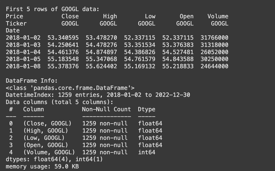

The googl_data.head() command shows the top rows, giving us a quick look at the columns available (Open, High, Low, Close, Adj Close, Volume) and their data types. googl_data.info() provides a more detailed summary, including the number of entries, non-null counts for each column, and memory usage. This helps confirm that we have a complete time series without missing values for our chosen column. For our analysis, we will focus on the Close price.

# Select only the 'Close' price and convert to a NumPy array for easier processing
googl_close_prices = googl_data['Close'].values

We extract the Close column from the DataFrame and convert it into a NumPy array. While pandas Series are highly functional, many statistical functions and NumPy operations work directly with arrays, which can sometimes be more efficient.

Visualizing the Raw GOOGL Closing Prices

The first step in any time series analysis is to visualize the data. This helps us identify trends, seasonality, and variance changes by simple inspection, which are all indicators of non-stationarity.

# Plot the raw GOOGL closing prices
plt.figure(figsize=(14, 7)) # Set a larger figure size for better readability
plt.plot(googl_data.index, googl_close_prices, label='GOOGL Close Price')
plt.title('GOOGL Stock Closing Prices (Raw Data)')
plt.xlabel('Date')
plt.ylabel('Price (USD)')
plt.grid(True) # Add a grid for easier reading of values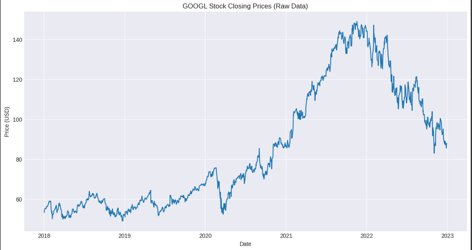

This code chunk initializes a plot, sets its size, and then plots the googl_close_prices against their corresponding dates (from googl_data.index). We add a title, axis labels, and a grid to make the plot informative.

Financial time series, especially stock prices, often exhibit a clear upward or downward trend over long periods, and their variance might also change (e.g., larger price swings when prices are higher). This visual pattern strongly suggests non-stationarity.

# Improve x-axis date formatting for better readability
plt.xticks(rotation=45) # Rotate date labels for better fit
plt.autofmt_xdate()    # Automatically format x-axis labels for dates
plt.tight_layout()     # Adjust layout to prevent labels from overlapping
plt.show()             # Display the plot

These lines enhance the plot’s readability. plt.xticks(rotation=45) rotates the date labels, preventing them from overlapping, especially when there are many data points. plt.autofmt_xdate() automatically applies smart formatting to date labels, and plt.tight_layout() adjusts plot parameters for a tight layout, minimizing whitespace and preventing labels from being cut off.

Looking at the plot, GOOGL’s closing prices clearly show an upward trend and possibly increasing variance over time. This visual inspection suggests that the series is non-stationary, which is a common characteristic of financial asset prices.

Testing for Stationarity with the ADF Test (Raw Data)

To formally test for stationarity, we employ the Augmented Dickey-Fuller (ADF) test. As discussed in Section 3.2.2, the null hypothesis of the ADF test is that the time series has a unit root, meaning it is non-stationary. If the p-value is below our chosen significance level (e.g., 0.05), we reject the null hypothesis and conclude the series is stationary.

To make our code cleaner and reusable, let’s define a function to perform and print the results of the ADF test.

def perform_adf_test(series, name='Time Series'):
    """
    Performs the Augmented Dickey-Fuller test on a given time series
    and prints the results.Parameters:
    series (array-like): The time series data to test.
    name (str): A descriptive name for the series being tested.
    """
    print(f"\n--- Augmented Dickey-Fuller Test Results for {name} ---")
    # Perform ADF test
    result = adfuller(series)
    adf_statistic = result[0]
    p_value = result[1]
    critical_values = result[4]
    # Print results
    print(f'ADF Statistic: {adf_statistic:.4f}')
    print(f'P-value: {p_value:.4f}')
    print('Critical Values:')
    for key, value in critical_values.items():
        print(f'   {key}: {value:.4f}')
    # Interpret the results
    if p_value <= 0.05:
        print(f"Conclusion: P-value ({p_value:.4f}) is <= 0.05. Reject the Null Hypothesis.")
        print(f"            The {name} series is likely stationary.")
    else:
        print(f"Conclusion: P-value ({p_value:.4f}) is > 0.05. Fail to Reject the Null Hypothesis.")
        print(f"            The {name} series is likely non-stationary.")
    print("--------------------------------------------------")

This perform_adf_test function encapsulates the logic for running the adfuller test and interpreting its output. It takes the time series data and an optional name as input, then neatly prints the ADF statistic, p-value, and critical values. Critically, it provides a clear conclusion based on the p-value against a 0.05 significance level. This function will be reused multiple times, demonstrating good programming practice.

Now, let’s apply this function to our raw GOOGL closing prices:

# Apply ADF test to the raw GOOGL closing prices
perform_adf_test(googl_close_prices, name='Raw GOOGL Close Prices')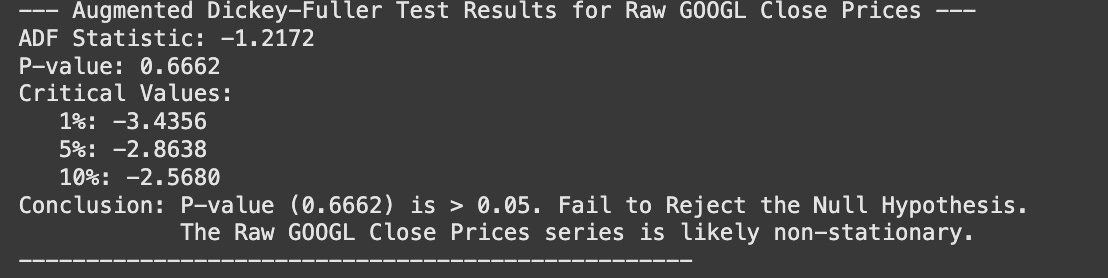

As expected from the visual inspection, the ADF test for the raw GOOGL close prices will likely yield a high p-value (e.g., > 0.05), leading us to fail to reject the null hypothesis. This confirms that the raw GOOGL closing price series is non-stationary, meaning it has a unit root. This is a characteristic feature of a random walk.

Differencing the Data

Since the raw GOOGL prices are non-stationary, we need to transform them to achieve stationarity before applying many time series models. For a random walk, the first difference is expected to be stationary and resemble white noise.

We use numpy.diff to compute the first-order difference.

# Compute the first-order difference of the GOOGL closing prices
# np.diff returns an array of n-1 elements if input has n elements
googl_differenced = np.diff(googl_close_prices)
# Since differencing reduces the length by 1, we adjust the index for plotting
# We align the differenced data with the original index starting from the second element
googl_differenced_index = googl_data.index[1:]

np.diff(series) calculates the difference between consecutive elements: series[i] - series[i-1]. This operation effectively removes a linear trend. For a random walk, which is defined by Y_t = Y_{t-1} + e_t, the first difference Y_t - Y_{t-1} = e_t should be white noise, which is a stationary process. Note that np.diff returns an array one element shorter than the input, so we adjust the index accordingly for future plotting and analysis.

Now, let’s visualize the differenced GOOGL prices. This plot should look very different from the raw price plot; it should fluctuate around zero without a clear trend or changing variance.

# Plot the differenced GOOGL closing prices
plt.figure(figsize=(14, 7))
plt.plot(googl_differenced_index, googl_differenced, label='Differenced GOOGL Close Price', color='orange')
plt.title('Differenced GOOGL Stock Closing Prices (First Difference)')
plt.xlabel('Date')
plt.ylabel('Price Change (USD)')
plt.grid(True)
plt.xticks(rotation=45)
plt.autofmt_xdate()
plt.tight_layout()
plt.show()

The plot of the differenced series now shows fluctuations around a constant mean (zero), and the variance appears relatively constant over time. This visual characteristic strongly suggests that the differenced series is stationary. Compare this to the upward-trending raw price plot; the transformation has effectively removed the trend and stabilized the mean.

Testing for Stationarity with the ADF Test (Differenced Data)

After differencing, we should re-run the ADF test to formally confirm that the series has become stationary.

# Apply ADF test to the differenced GOOGL closing prices
perform_adf_test(googl_differenced, name='Differenced GOOGL Close Prices')

For the differenced GOOGL prices, we expect the ADF test to yield a very low p-value (e.g., much less than 0.05). This result would lead us to reject the null hypothesis of a unit root, confirming that the differenced series is indeed stationary. This is a crucial step in identifying a random walk, as the first difference of a random walk is stationary.

Analyzing Autocorrelation with ACF Plots

The final diagnostic tool for identifying a random walk is the Autocorrelation Function (ACF) plot. For a random walk, the raw series will exhibit significant, slowly decaying autocorrelation. However, the first difference of a random walk should have no significant autocorrelation, except potentially at lag 0 (which is always 1) and possibly a few isolated spikes due to pure chance.

First, let’s look at the ACF of the raw GOOGL closing prices to see the characteristic slow decay of a non-stationary series.

# Plot ACF for raw GOOGL closing prices
plt.figure(figsize=(10, 6))
plot_acf(googl_close_prices, lags=40, ax=plt.gca(), title='Autocorrelation Function (ACF) for Raw GOOGL Close Prices')
plt.xlabel('Lag')
plt.ylabel('Autocorrelation')
plt.grid(True)
plt.show()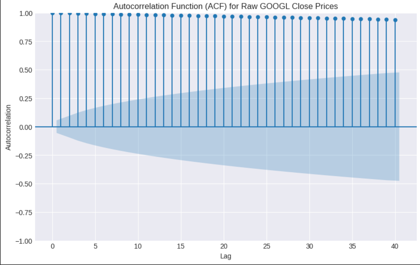

The ACF plot of the raw GOOGL prices clearly shows strong, positive autocorrelation that decays very slowly. This slow decay is a hallmark of a non-stationary time series with a trend or unit root, further supporting our ADF test results for the raw data.

Now, let’s examine the ACF of the differenced GOOGL closing prices. If GOOGL prices are a random walk, the differenced series should resemble white noise, meaning its ACF plot should show no significant autocorrelation at any lag (except lag 0).

# Plot ACF for differenced GOOGL closing prices
plt.figure(figsize=(10, 6))
plot_acf(googl_differenced, lags=40, ax=plt.gca(), title='Autocorrelation Function (ACF) for Differenced GOOGL Close Prices')
plt.xlabel('Lag')
plt.ylabel('Autocorrelation')
plt.grid(True)
plt.show()

In this ACF plot for the differenced GOOGL prices, we observe a dramatic change. Most of the autocorrelation coefficients fall within the blue shaded region, which represents the 95% confidence interval. This means that any spikes outside this region are statistically significant at the 5% level.

Interpreting Isolated Spikes: It’s common to see one or two isolated spikes outside the confidence interval in the ACF of a series that is otherwise considered white noise. This is due to the nature of statistical significance testing. At a 95% confidence level, we expect approximately 5% of the lags to appear “significant” purely by chance, even if the true underlying process is white noise. For example, if we plot 40 lags, we might expect around 40 * 0.05 = 2 lags to cross the confidence bounds randomly. Therefore, unless there’s a clear pattern of multiple consecutive significant lags, or a very strong spike, isolated significant lags are generally disregarded as random fluctuations.

In the case of differenced GOOGL prices, you will likely see that there are very few, if any, significant spikes beyond lag 0. This indicates that all historical information has been captured by the previous period’s price, and the current price change is essentially unpredictable, resembling white noise.

Synthesizing the Conclusion: Is GOOGL a Random Walk?

Based on our comprehensive analysis:

1. Visual Inspection of Raw Prices: The raw GOOGL closing prices show a clear upward trend and possibly changing variance, indicating non-stationarity.

2. ADF Test on Raw Prices: The ADF test confirms non-stationarity (high p-value, fail to reject null hypothesis of unit root).

3. Visual Inspection of Differenced Prices: The first-differenced GOOGL prices fluctuate around a constant mean (zero) with stable variance, appearing stationary.

4. ADF Test on Differenced Prices: The ADF test on the differenced prices confirms stationarity (low p-value, reject null hypothesis).

5. ACF of Raw Prices: The ACF of the raw prices shows strong, slowly decaying autocorrelation, characteristic of a non-stationary series.

6. ACF of Differenced Prices: The ACF of the differenced prices shows no significant autocorrelation beyond lag 0, consistent with white noise, after accounting for chance spikes.

The combined evidence strongly suggests that GOOGL stock prices exhibit the characteristics of a random walk. This means that the best prediction for tomorrow’s price is today’s price, plus some random noise.

Implications for Forecasting

The identification of GOOGL as a random walk has profound implications for forecasting:

• Efficient Market Hypothesis (EMH): This finding aligns with the Weak-form Efficient Market Hypothesis, which states that all past market prices and volume data are fully reflected in current prices. If stock prices follow a random walk, it implies that it’s impossible to consistently “beat the market” using only historical price data because price changes are essentially unpredictable.

• Naive Forecasting: For a random walk, the optimal forecast for the next period’s value is simply the current period’s value. Any more complex model (e.g., ARIMA, machine learning) attempting to predict future price changes based on past price changes would likely perform no better than this simple “naive” forecast. This doesn’t mean stock prices are entirely unpredictable; it means that price changes are unpredictable based on their own past. Other factors (economic news, company earnings, sentiment) might still influence prices.

• Model Selection: If a financial series is a random walk, traditional time series models that rely on past patterns (like AR, MA, or ARIMA models with AR or MA components) would not be appropriate for forecasting the level of the series. Instead, differencing would be necessary to achieve stationarity, and then the focus would shift to modeling the white noise process of the differenced series, which essentially means there’s no pattern to model.

While many financial time series (like stock prices, exchange rates) are often approximated as random walks, it’s important to remember that not all economic or financial data exhibit this behavior. For instance, interest rates, inflation, or commodity prices might display different time series properties that require more complex models. The systematic approach of visual inspection, stationarity testing, differencing, and ACF analysis is a fundamental skill for any time series analyst.

Forecasting a Random Walk

Having established the characteristics and identification methods for random walk processes, we now turn our attention to the crucial question of forecasting. While the concept of “forecasting” typically implies predicting future values based on discernible patterns, random walks present a unique challenge due to their inherent unpredictability.

The Unpredictability of Random Walks

A random walk process, as we’ve defined, can be expressed as:

Yt = Yt − 1 + ϵt

Where Yt is the value at time t, Yt − 1 is the value at the previous time step, and ϵt is a white noise error term with a mean of zero and constant variance. This formulation implies that the current value is simply the previous value plus a random shock.

The critical insight for forecasting a random walk stems from the properties of this error term. Since ϵt is white noise, it is by definition uncorrelated with past values of itself and past values of Yt. This lack of correlation means there is no linear relationship between past observations and the future random shock. Consequently, there’s no way to predict the direction or magnitude of the next step’s random movement.

This fundamental characteristic renders traditional statistical learning models (such as ARIMA models with autoregressive or moving average components, or more complex machine learning models) largely unsuitable for forecasting a pure random walk. These models rely on identifying and leveraging patterns, autocorrelations, or dependencies within the time series data. When such patterns are absent, as is the case with a random walk, these models have nothing substantial to learn from. Trying to force a complex model onto a random walk is akin to trying to predict the outcome of a fair coin flip — the best you can do is guess, and your guess will be right 50% of the time, regardless of how sophisticated your “model” is.

For a random walk, the optimal forecast for the next value, or indeed any future value, is simply the last observed value. Any deviation from this would imply that you believe you can predict the random shock ϵt, which contradicts its definition as unpredictable white noise.

Naive Forecasting: The Best Bet

Given the inherent unpredictability of random walks, the most appropriate and often the most accurate forecasting methods are surprisingly simple: the “naive” approaches. These methods serve as crucial baselines, especially for series where complex patterns are absent. For a random walk, a specific naive method stands out as the theoretically optimal choice.

The Last Value Forecast

The “last value” or “naive” forecast simply states that the best prediction for any future time step is the most recently observed value. For a random walk, this is not just a simplistic approach; it is the theoretically optimal forecast in terms of minimizing mean squared error. Why? Because any deviation from the last observed value would require predicting the future random shock, which is impossible.

Let’s illustrate this with a small numerical example. Imagine a simplified random walk sequence:

TimeValue110021013994102

If our last observed value is 102 at Time 4, then our last value forecast for Time 5 would simply be 102. The same forecast (102) would apply for Time 6, Time 7, and so on.

Now, let’s implement this in Python. We’ll start by generating a simple synthetic random walk to demonstrate the concept.

import numpy as np
import pandas as pd
import matplotlib.pyplot as plt
# Set a random seed for reproducibility
np.random.seed(42)
# Generate a synthetic random walk
# Start value
initial_value = 100
# Number of steps
n_steps = 100
# Generate random steps (white noise)
random_steps = np.random.normal(loc=0, scale=1, size=n_steps)
# Calculate the random walk path
# Cumulative sum of random steps added to initial value
synthetic_random_walk = initial_value + np.cumsum(random_steps)
# Create a Pandas Series for easier handling
rw_series = pd.Series(synthetic_random_walk, name="Synthetic Random Walk")
print("First 5 values of the synthetic random walk:")
print(rw_series.head())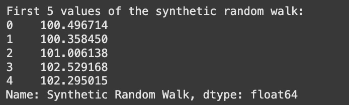

In this first code segment, we set up a controlled environment by fixing a random seed, which ensures that our generated “random” walk is reproducible. We then define an initial_value and n_steps to create a sequence. The core of the random walk generation is np.random.normal(loc=0, scale=1, size=n_steps), which produces the white noise error terms (ϵt). Finally, np.cumsum adds these random steps cumulatively to the initial value, simulating the Yt = Yt − 1 + ϵt behavior. We store this in a Pandas Series for convenient time series operations.

Next, we’ll implement the last value forecast for this synthetic series.

# Function to perform last value forecasting
def forecast_last_value(series, horizon=1):
    """
    Performs a last value (naive) forecast for a given series.Args:
        series (pd.Series): The input time series.
        horizon (int): The number of future steps to forecast.
    Returns:
        pd.Series: Forecasted values for the specified horizon.
    """
    if series.empty:
        return pd.Series([])
    # The last observed value is our forecast for all future steps
    last_val = series.iloc[-1]
    # Create a Pandas Series for the forecasted values
    # The index should extend beyond the original series
    last_index = series.index[-1]
    forecast_index = pd.RangeIndex(start=last_index + 1, stop=last_index + 1 + horizon)
    
    # All forecasted values are the last observed value
    forecasts = pd.Series([last_val] * horizon, index=forecast_index, name="Last Value Forecast")
    return forecasts
# Apply the last value forecast to our synthetic random walk
forecast_horizon = 5
rw_last_value_forecast = forecast_last_value(rw_series, horizon=forecast_horizon)
print(f"\nLast {forecast_horizon} values of the synthetic random walk:")
print(rw_series.tail(forecast_horizon))
print(f"\nLast Value Forecast for the next {forecast_horizon} steps:")
print(rw_last_value_forecast)

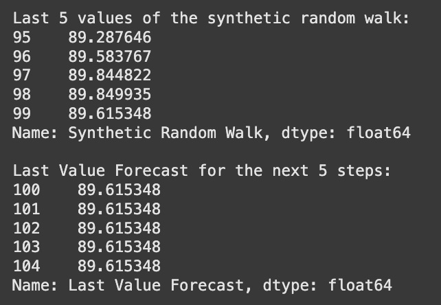
This segment defines a reusable function forecast_last_value. The function takes a time series and a horizon (how many steps into the future to predict). The core logic is series.iloc[-1], which retrieves the very last data point. This single value then becomes the forecast for all horizon steps. We also ensure that the forecasted series has an appropriate index, extending beyond the original data’s index, which is crucial for plotting and alignment. The output clearly shows that all future predictions are identical to the last observed value.

Now, let’s apply this to our GOOGL data. We’ll assume you have loaded the GOOGL_data.csv and processed it to have a Close price series as demonstrated in previous sections. For this example, we’ll simulate a portion of GOOGL’s closing prices if the actual data isn’t directly available in this environment.

# Assuming GOOGL_data is available from previous sections.
# If not, let's create a placeholder for demonstration purposes
try:
    # This assumes 'googl_df' is a DataFrame with a 'Close' column
    # from previous sections, indexed by date.
    googl_close_prices = googl_df['Close']
except NameError:
    print("\n'googl_df' not found, creating a synthetic GOOGL-like series for demonstration.")
    # Create a synthetic GOOGL-like random walk for demonstration
    # This simulates a stock price for a short period
    start_date = '2023-01-01'
    dates = pd.date_range(start=start_date, periods=252, freq='B') # 252 business days in a year
    
    # Simulate a stock price random walk
    np.random.seed(43) # Another seed for this specific simulation
    initial_googl_price = 100.0
    daily_returns = np.random.normal(loc=0.0005, scale=0.01, size=len(dates)) # Small positive drift, some volatility
    simulated_prices = initial_googl_price * np.exp(np.cumsum(daily_returns))
    
    googl_close_prices = pd.Series(simulated_prices, index=dates, name="GOOGL Close Price")
print("\nLast 5 GOOGL Close Prices:")
print(googl_close_prices.tail())
# Apply the last value forecast to GOOGL data
googl_forecast_horizon = 10 # Forecast for the next 10 trading days
googl_last_value_forecast = forecast_last_value(googl_close_prices, horizon=googl_forecast_horizon)
print(f"\nGOOGL Last Value Forecast for the next {googl_forecast_horizon} steps:")
print(googl_last_value_forecast)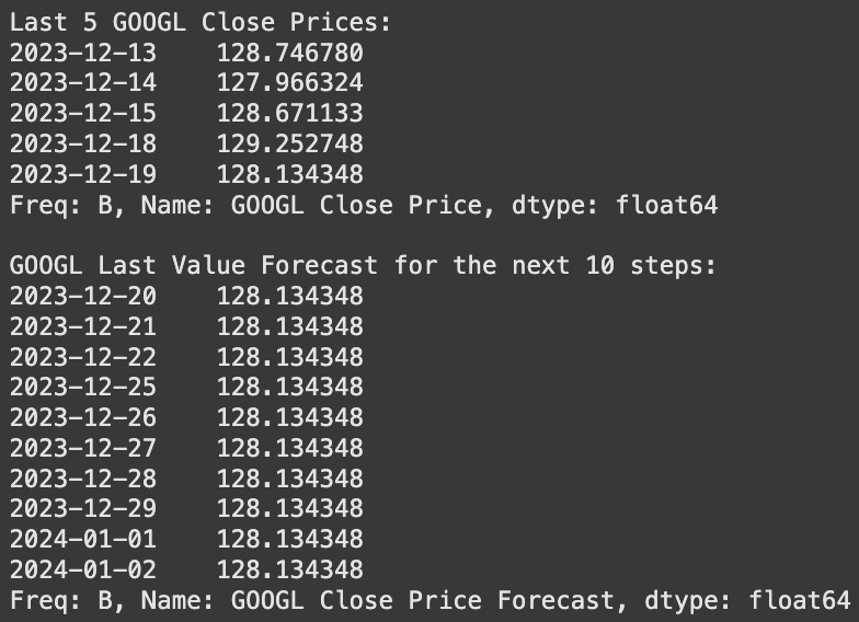

In this final last-value forecasting code block, we first attempt to use a googl_df that would have been loaded in previous sections. If it’s not found (e.g., if running this code in isolation), a synthetic googl_close_prices series is generated, mimicking typical stock price behavior as a random walk with a slight positive drift. This ensures the example remains runnable and illustrative. We then apply our forecast_last_value function to this GOOGL data, demonstrating how straightforward it is to generate the optimal forecast for a random walk.

The Historical Mean Forecast (and its limitations for Random Walks)

Another naive forecasting method is the “historical mean” forecast, where the prediction for any future value is simply the average of all past observed values. This method is appropriate for time series that are stationary around a constant mean, meaning they tend to fluctuate around a fixed average over time without any long-term trend or seasonality.

However, a random walk is not stationary around a constant mean. By definition, a random walk has a drifting mean and increasing variance over time. If you calculate the mean of a random walk, it will change significantly as more data points are added, especially if the random walk has drifted far from its starting point. Therefore, using the historical mean to forecast a random walk is generally a poor choice and will likely lead to large forecast errors. It’s crucial to understand why this method is unsuitable for random walks, even though it’s a “naive” method. It serves as a good contrast to highlight the specific properties of random walks.

Let’s implement the historical mean forecast and then compare it with the last value forecast.

# Function to perform historical mean forecasting
def forecast_historical_mean(series, horizon=1):
    """
    Performs a historical mean forecast for a given series.Args:
        series (pd.Series): The input time series.
        horizon (int): The number of future steps to forecast.
    Returns:
        pd.Series: Forecasted values for the specified horizon.
    """
    if series.empty:
        return pd.Series([])
    # Calculate the mean of all observed values
    historical_mean = series.mean()
    # Create a Pandas Series for the forecasted values
    last_index = series.index[-1]
    forecast_index = pd.RangeIndex(start=last_index + 1, stop=last_index + 1 + horizon)
    
    # All forecasted values are the historical mean
    forecasts = pd.Series([historical_mean] * horizon, index=forecast_index, name="Historical Mean Forecast")
    return forecasts
# Apply the historical mean forecast to our synthetic random walk
rw_historical_mean_forecast = forecast_historical_mean(rw_series, horizon=forecast_horizon)
print(f"\nHistorical Mean Forecast for the next {forecast_horizon} steps:")
print(rw_historical_mean_forecast)

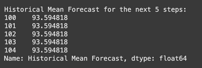
This forecast_historical_mean function is similar in structure to the last value forecast, but instead of taking the last value, it computes the series.mean()of all available data points. This mean then becomes the forecast for all future steps. For a random walk, where the series can drift away from its starting point, this mean will likely be quite different from the last observed value, leading to less accurate forecasts.

Now, let’s apply it to our GOOGL data and visually compare both naive forecasts.

# Apply the historical mean forecast to GOOGL data
googl_historical_mean_forecast = forecast_historical_mean(googl_close_prices, horizon=googl_forecast_horizon)
print(f"\nGOOGL Historical Mean Forecast for the next {googl_forecast_horizon} steps:")
print(googl_historical_mean_forecast)
# --- Visual Comparison of Forecasts ---
# Combine original data and forecasts for plotting
# Take a recent segment of the original data for better visualization
plot_series = googl_close_prices.tail(30) # Last 30 actual values
combined_series = pd.concat([plot_series, googl_last_value_forecast, googl_historical_mean_forecast])
plt.figure(figsize=(12, 6))
plt.plot(plot_series.index, plot_series.values, label='Actual GOOGL Close Prices (Recent)', color='blue')
plt.plot(googl_last_value_forecast.index, googl_last_value_forecast.values, 
         label='Last Value Forecast', color='green', linestyle='--')
plt.plot(googl_historical_mean_forecast.index, googl_historical_mean_forecast.values, 
         label='Historical Mean Forecast', color='red', linestyle=':')
plt.title('GOOGL Close Price: Actual vs. Naive Forecasts')
plt.xlabel('Date')
plt.ylabel('Price')
plt.legend()
plt.grid(True)
plt.show()

The final code block applies the historical mean forecast to the GOOGL data. Crucially, it then generates a plot to visually compare the actual GOOGL prices with both the last value forecast and the historical mean forecast. This visual representation vividly demonstrates why the last value forecast is superior for a random walk: it starts exactly where the series left off, while the historical mean forecast might be significantly off, especially if the random walk has exhibited a strong trend. This plot helps solidify the understanding of the limitations of the historical mean for random walks.

Understanding the Forecasting Horizon

The concept of a “forecasting horizon” refers to how far into the future we are trying to predict. For a time series that exhibits predictable patterns, a longer forecasting horizon generally leads to increased uncertainty in the predictions, but the model might still capture underlying trends or seasonalities. For a pure random walk, however, the implications of the forecasting horizon are distinct and critical:

1. Best Forecast is Always the Last Value: For a pure random walk, the best forecast for any future time step (whether it’s the next day, next week, or next month) is simply the last observed value. As we’ve discussed, there’s no information in the past to predict the direction of the next random shock. Therefore, Ft + 1 = Yt, Ft + 2 = Yt, and so on. The forecast line for a random walk is a flat line extending from the last data point.

2. Uncertainty Grows with Horizon: While the point forecast remains the last observed value, the uncertainty around that forecast grows proportionally with the square root of the forecasting horizon. The variance of the forecast error for a random walk is h × σ2, where h is the horizon and σ2 is the variance of the white noise error term (ϵt). This means that although our best guess is always the last value, our confidence in that guess diminishes rapidly as we look further into the future. The range of possible outcomes widens significantly.

This increasing uncertainty implies that while you can provide a point forecast for a random walk for any horizon, the practical utility of long-term forecasts is very limited. For instance, predicting GOOGL’s closing price for tomorrow based on today’s close might be reasonable (it’s the best you can do), but predicting its price a year from now based on today’s close is almost meaningless due to the massive potential deviation from that single point forecast.

In financial markets, this concept is crucial. Stock prices are often modeled as random walks (or close approximations), implying that short-term price movements are inherently unpredictable. This is a core tenet of the Efficient Market Hypothesis in its weakest form. Traders and investors often rely on fundamental analysis or very short-term technical analysis, but the idea of accurately predicting long-term price levels for individual stocks is generally viewed with skepticism within the realm of quantitative finance, precisely because of their random walk characteristics.

Forecasting on a Long Horizon

Having established the characteristics of random walks and identified them in time series data, the natural next step for a trader or analyst is to consider how to forecast such processes. This section delves into the practical aspects of forecasting random walks, specifically focusing on simple, yet often the most appropriate, “naive” methods, and evaluating their performance over a long forecasting horizon. Understanding the limitations of forecasting for random walks is crucial, as it prevents the misapplication of more complex models and sets realistic expectations for prediction accuracy.

Preparing Data for Time Series Forecasting

Before applying any forecasting method, it’s essential to properly prepare the time series data. For evaluating forecast accuracy, we typically split our data into a training set and a testing set. The model learns from the training data, and its performance is then assessed on the unseen testing data. For time series, this split must be chronological to simulate real-world conditions, meaning we train on past data and forecast into the future.

First, let’s ensure we have a simulated random walk to work with. This example uses a simple random walk, where each step is a random increment from the previous value.

import numpy as np
import pandas as pd
import matplotlib.pyplot as plt
from sklearn.metrics import mean_squared_error
# Set a seed for reproducibility to ensure consistent results
np.random.seed(42)
# Simulate a random walk
initial_value = 0
num_steps = 1000
# Generate random steps (e.g., daily price changes) from a normal distribution
steps = np.random.normal(loc=0, scale=1, size=num_steps)
# The random walk is the cumulative sum of these steps plus the initial value
random_walk = initial_value + np.cumsum(steps)
# Create a Pandas DataFrame for easy manipulation
# We use a simple integer index representing time steps for this simulation
df = pd.DataFrame({'value': random_walk})
print("Simulated Random Walk Data Head:")
print(df.head())
print("\nSimulated Random Walk Data Tail:")
print(df.tail())

The code above initializes our environment by importing necessary libraries and then generates a simulated random walk. We start with an initial_value and then cumulatively sum num_steps of normally distributed random increments. This creates a series where each step is the previous value plus a random shock, perfectly embodying the definition of a random walk. The data is then stored in a Pandas DataFrame, which is a standard structure for time series analysis. This simulation helps us understand the behavior of financial series that often approximate random walks, such as certain stock prices or exchange rates.

Next, we perform the train-test split. For time series, this is typically a rolling or expanding window, but for simplicity here, we’ll use a fixed percentage. We’ll use 80% of the data for training and the remaining 20% for testing.

# Define the split point for train and test sets
train_size = int(len(df) * 0.8)
# Split the DataFrame into training and testing sets chronologically
train, test = df[0:train_size], df[train_size:len(df)]
# Determine the number of steps in the forecast horizon
forecast_horizon = len(test)
# Capture the index (time steps) for the forecast horizon, useful for plotting
test_index = test.index
print(f"\nTraining set size: {len(train)} observations")
print(f"Testing set size: {len(test)} observations (Forecast Horizon)")
print(f"First 5 values of training set:\n{train.head()}")
print(f"First 5 values of testing set:\n{test.head()}")

Here, train_size determines the cut-off point. We slice the DataFrame df using integer-location based indexing to create train and test DataFrames.forecast_horizon represents the number of future steps we need to predict. This setup ensures that our ‘model’ (naive methods in this case) only sees data up to the train_size index, and then makes predictions for test_index. This mirrors a real-world scenario where you train a model on historical data and then use it to predict future, unseen values.

Naive Forecasting Methods for Random Walks

Given the inherent unpredictability of a true random walk — where past movements offer no predictive power for future changes — complex forecasting models often perform no better than simple, “naive” benchmarks. In fact, for a pure random walk, these naive methods are theoretically the optimal point forecasts. They serve as crucial baselines against which any more sophisticated model must be compared. If a complex model cannot outperform these simple baselines, it suggests that the series is either a random walk or that the model is not capturing any meaningful patterns.

We’ll explore three common naive forecasting strategies: the historical mean, the last known value, and the drift method. To promote modularity and reusability, we will encapsulate each method within its own function.

Historical Mean Forecast

The historical mean forecast predicts that all future values will be equal to the average of all observed values in the training set. This method assumes that the time series is stationary around a constant mean. While a pure random walk is not stationary, this method still serves as a fundamental, albeit often poor, baseline.

def historical_mean_forecast(train_data, horizon):
    """
    Calculates the historical mean from the training data and
    uses it as a constant forecast for the given horizon.Args:
        train_data (pd.DataFrame): The training data (e.g., historical prices).
        horizon (int): The number of steps to forecast into the future.
    Returns:
        np.array: An array of constant forecasts, each equal to the historical mean.
    """
    # Calculate the mean of the 'value' column from the training data
    mean_value = np.mean(train_data['value'])
    # Create an array where every element is this mean value, for the length of the horizon
    return np.full(horizon, mean_value)
# Apply the historical mean forecast to our test set
test['mean_forecast'] = historical_mean_forecast(train, forecast_horizon)
print("\nTest data with Historical Mean Forecast (first 5 rows of test set):")
print(test.head())

The historical_mean_forecast function calculates the mean of the value column from the train_data. It then uses np.full to create an array of thismean_value repeated for the entire forecast_horizon. This array is then assigned to a new column, mean_forecast, in our test DataFrame. This method essentially assumes the process will revert to its long-term average, which is a strong assumption for a non-stationary series like a random walk, often leading to large errors.

Last Known Value Forecast

The last known value forecast (often called the “Naive Forecast” or “Random Walk Forecast”) simply predicts that the next value will be the same as the last observed value. For a pure random walk, where the best estimate of the next value is the current value (because changes are unpredictable, having a mean of zero), this method often performs surprisingly well, especially for short horizons. It effectively predicts that the change from the last known value will be zero.

def last_value_forecast(train_data, horizon):
    """
    Uses the last observed value from the training data as a constant forecast
    for the given horizon.Args:
        train_data (pd.DataFrame): The training data.
        horizon (int): The number of steps to forecast.
    Returns:
        np.array: An array of constant forecasts based on the last value.
    """
    # Get the very last value from the 'value' column of the training data
    last_value = train_data['value'].iloc[-1]
    # Create an array where every element is this last value, for the length of the horizon
    return np.full(horizon, last_value)
# Apply the last known value forecast
test['last_value_forecast'] = last_value_forecast(train, forecast_horizon)
print("\nTest data with Last Known Value Forecast (first 5 rows of test set):")
print(test.head())

The last_value_forecast function retrieves the final value from the train_data using iloc[-1]. Similar to the mean forecast, np.full is then used to extend this single value across the entire forecast_horizon, populating the last_value_forecast column in the test DataFrame. This approach is particularly sensible for random walks because their “memory” is only of the most recent state; past changes don’t inform future ones, making the current value the best predictor of the next.

Drift Method Forecast

The drift method is a slightly more sophisticated naive forecast. It accounts for a constant average increase or decrease (the “drift”) observed in the historical data and projects this trend into the future. This method is particularly relevant when dealing with a “random walk with drift” (as discussed in Equation 3.1: Yt = C + Yt − 1 + ϵt), where the series tends to increase or decrease by a small constant amount on average at each step, in addition to the random shock (ϵt). The drift method estimates this constant C from the training data and adds it cumulatively to the last observed value.

def drift_forecast(train_data, horizon):
    """
    Calculates the average change (drift) from the training data
    and extrapolates it from the last observed value.Args:
        train_data (pd.DataFrame): The training data.
        horizon (int): The number of steps to forecast.
    Returns:
        np.array: An array of forecasts based on the drift method.
    """
    # Calculate the average change per step (drift) from the training data.
    # The first difference of the series represents the steps in the random walk.
    drift = train_data['value'].diff().mean()
    # Get the last observed value from the training data
    last_value = train_data['value'].iloc[-1]
    # Project the drift into the future.
    # For each step in the horizon, add the cumulative drift to the last observed value.
    forecast_values = [last_value + (drift * (i + 1)) for i in range(horizon)]
    return np.array(forecast_values)
# Apply the drift forecast
test['drift_forecast'] = drift_forecast(train, forecast_horizon)
print("\nTest data with Drift Forecast (first 5 rows of test set):")
print(test.head())

The drift_forecast function first calculates the average drift by taking the mean of the first differences of the training data (train_data['value'].diff().mean()). This directly estimates the constant C from the random walk with drift model. It then takes the last_value from the training set and projects future values by cumulatively adding the calculated drift for each step in the forecast_horizon. This method implicitly assumes that the underlying systematic trend observed in the past will continue into the future. For financial time series like stock prices, which sometimes exhibit a slight positive long-term drift, this can be a more reasonable baseline than simply the last value.

Visualizing Forecasts

Visualization is a critical step in understanding forecast performance. Plotting the actual values against the predictions allows for quick qualitative assessment of how well each method captures the series’ behavior. For random walks, this visual inspection will quickly highlight the futility of long-term predictions.

# Plotting the forecasts
fig, ax = plt.subplots(figsize=(12, 6))
# Plot training data (historical data used for training)
ax.plot(train.index, train['value'], label='Training Data (Actual)', color='blue')
# Plot actual test data (the true future values)
ax.plot(test.index, test['value'], label='Test Data (Actual)', color='black', linestyle='--')
# Plot each of the naive forecasts
ax.plot(test_index, test['mean_forecast'], label='Mean Forecast', color='red', linestyle=':')
ax.plot(test_index, test['last_value_forecast'], label='Last Value Forecast', color='green', linestyle='-.')
ax.plot(test_index, test['drift_forecast'], label='Drift Forecast', color='purple', linestyle='-')
# Highlight the forecast region with a shaded vertical span
ax.axvspan(train.index.max(), test.index.max(), color='#cccccc', alpha=0.5, label='Forecast Horizon')
ax.set_title('Random Walk Forecasting with Naive Methods')
ax.set_xlabel('Time Step')
ax.set_ylabel('Value')
ax.legend() # Display the legend to identify lines
plt.grid(True, linestyle='--', alpha=0.6) # Add a grid for better readability
plt.tight_layout() # Adjust layout to prevent labels from overlapping
# Save the plot to a file for future reference
plt.savefig('random_walk_naive_forecasts.png', dpi=300)
plt.show()

This plotting code generates a comprehensive visualization. It first plots the train data (what the models learned from) and the test data (the actual values the models are trying to predict). Then, it overlays the predictions from each of our three naive methods: mean_forecast, last_value_forecast, and drift_forecast. The ax.axvspan function visually delineates the forecast horizon, making it clear which part of the plot represents predictions. The legend helps identify each line. Observing this plot, you will typically see that for a random walk, all forecasts quickly diverge from the actual values, especially over a longer horizon. The last_value_forecast and drift_forecast might track the actual path slightly better initially than the mean_forecast, but all will fail to capture the inherent randomness over time, demonstrating the challenge of forecasting such series.

Evaluating Forecast Performance with Error Metrics

Visual inspection provides qualitative insights, but quantitative metrics are essential for objective evaluation and comparison. For forecasting continuous values like stock prices, Mean Squared Error (MSE), Root Mean Squared Error (RMSE), and Mean Absolute Error (MAE) are commonly used.

Mean Squared Error (MSE), Root Mean Squared Error (RMSE), and Mean Absolute Error (MAE)

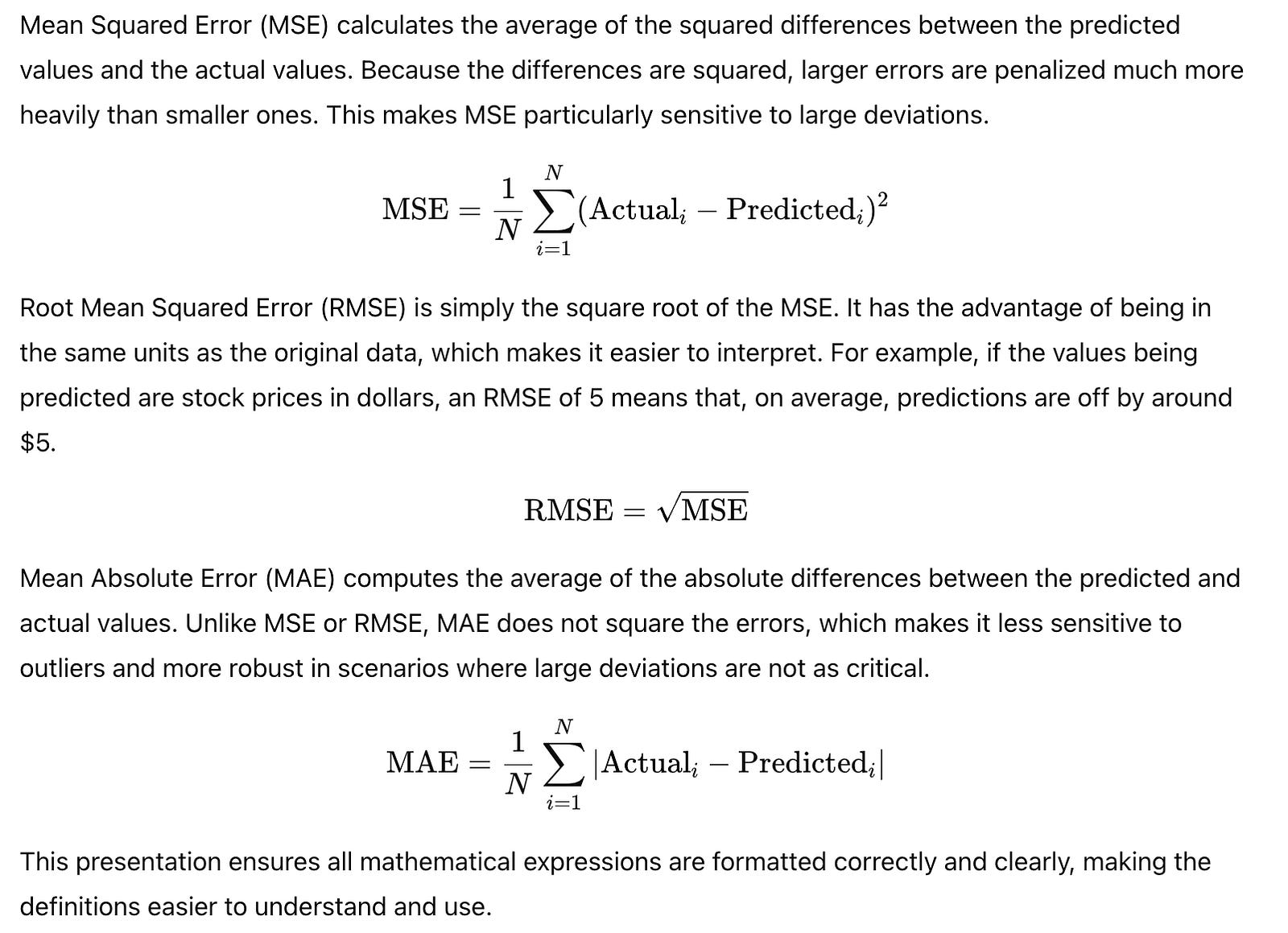
For random walks, metrics like Mean Absolute Percentage Error (MAPE) are generally unsuitable because the true value can be zero or close to zero (as in our simulated random walk which starts at zero), leading to division by zero or extremely large percentage errors. MSE and RMSE, focusing on the absolute magnitude of the error, are more robust in such scenarios.

Let’s calculate MSE and RMSE for each of our naive forecasts.

# Extract the actual values from the test set for comparison
actual_values = test['value']
print("Forecast Evaluation Metrics:")
# Evaluate the Mean Forecast
mse_mean = mean_squared_error(actual_values, test['mean_forecast'])
rmse_mean = np.sqrt(mse_mean)
# For completeness, let's also calculate MAE
mae_mean = np.mean(np.abs(actual_values - test['mean_forecast']))
print(f"Mean Forecast      - MSE: {mse_mean:.4f}, RMSE: {rmse_mean:.4f}, MAE: {mae_mean:.4f}")
# Evaluate the Last Value Forecast
mse_last = mean_squared_error(actual_values, test['last_value_forecast'])
rmse_last = np.sqrt(mse_last)
mae_last = np.mean(np.abs(actual_values - test['last_value_forecast']))
print(f"Last Value Forecast- MSE: {mse_last:.4f}, RMSE: {rmse_last:.4f}, MAE: {mae_last:.4f}")
# Evaluate the Drift Forecast
mse_drift = mean_squared_error(actual_values, test['drift_forecast'])
rmse_drift = np.sqrt(mse_drift)
mae_drift = np.mean(np.abs(actual_values - test['drift_forecast']))
print(f"Drift Forecast     - MSE: {mse_drift:.4f}, RMSE: {rmse_drift:.4f}, MAE: {mae_drift:.4f}")

The output of this code will typically show very high MSE and RMSE values for all naive methods, especially over a long forecast horizon. This is not an indication of poor implementation, but rather a direct consequence of the unpredictable nature of random walks. A high RMSE value, for example, might indicate that your forecasts are off by an average of X units, where X is a significant portion of the typical range of the series. For predictable series, you would aim for an RMSE that is small relative to the typical fluctuations of the data. For a random walk, the error will grow with the square root of the forecast horizon, meaning long-term predictions become increasingly unreliable. This demonstrates the inherent difficulty in predicting such series.

Implications for Long-Horizon Forecasting

The exercise of forecasting a random walk, particularly over a long horizon, starkly illustrates its inherent unpredictability. The key takeaways for traders and analysts are:

• No Long-Term Predictability: For a true random walk, past data provides no information about future directions or magnitudes of change. Any attempt to predict specific future values beyond the immediate next step is essentially futile. The error in prediction (RMSE) will grow proportionally to the square root of the forecast horizon. This means that while a forecast for the next day might be somewhat close, a forecast for a month or a year out will likely be wildly inaccurate.

• Naive Methods as Benchmarks: The simple naive forecasts (last value, drift) are not just “bad” forecasts; for a random walk, they are often the best possible point forecasts. Any more complex statistical or machine learning model (e.g., ARIMA, neural networks) applied to a true random walk will not yield significantly better point forecasts than these simple baselines. In fact, if a complex model does perform significantly better than these baselines on a series identified as a random walk, it might indicate that the series is not a pure random walk (e.g., it has some underlying pattern or stationarity that was overlooked), or that the model is overfitting to noise in the training data. This makes naive methods invaluable as a “sanity check” or “benchmark” against which any sophisticated model’s performance must be compared.

• Focus on Uncertainty, Not Point Forecasts: Given the high and ever-increasing error, providing a single point forecast for a random walk is misleading. Instead, the focus should shift to quantifying the uncertainty around the forecast, perhaps through prediction intervals. While not explicitly implemented here, conceptually, these intervals would widen significantly with the forecast horizon, reflecting the growing unpredictability. For a random walk, these intervals would grow as a cone, reflecting the increasing dispersion of possible future paths.

• Real-World Random Walks: Many financial time series, such as certain commodity prices, exchange rates, or even daily stock prices (when considering their log returns), often exhibit characteristics close to a random walk. This understanding is critical: if your financial asset is a random walk, your edge does not come from predicting its future price, but from managing risk, exploiting known market inefficiencies, or utilizing fundamental information outside of past price data. Trying to predict the unpredictable is a losing game.

This section underscores a fundamental principle in time series analysis: not all series are predictable. Recognizing a random walk allows you to set realistic expectations, avoid overfitting to noise, and focus on strategies that acknowledge inherent uncertainty rather than attempting to predict the unpredictable.

Forecasting the Next Timestep

In the previous section, we established that forecasting a random walk over a long horizon is inherently futile. The further out we try to predict, the more our forecast simply reverts to the historical mean, and the confidence intervals widen indefinitely, reflecting the process’s unpredictability. However, the situation changes when we consider forecasting just the immediate next timestep.

Recall the definition of a random walk:

Yt = Yt − 1 + ϵt

Where Yt is the value at time t, Yt − 1 is the value at the previous time step, and ϵt is a white noise term (unpredictable, with a mean of zero and constant variance).

Given this definition, what is the best possible forecast for Yt if we know Yt − 1? Since ϵt is unpredictable with a mean of zero, our best point estimate for Yt is simply Yt − 1. This is known as the naive forecast or the “last known value” forecast. It’s the simplest possible forecasting method, stating that the next value will be the same as the current value. While seemingly simplistic, for a random walk, it is the most appropriate strategy for a one-step-ahead prediction.

Understanding the shift() Operation

Before implementing this in Python, let’s clarify how we can obtain the “last known value” using pandas. The shift() method is perfectly suited for this. It moves data points by a specified number of periods along the axis.

Consider a very simple sequence of numbers:

import pandas as pd
# A short sequence of values
data_series = pd.Series([10, 12, 11, 15, 13])
print("Original Series:")
print(data_series)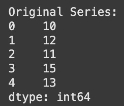

When we apply shift(periods=1), each value is moved down by one position. The first value in the new series will become NaN (Not a Number) because there’s no preceding value to shift into its position.

# Shifting by 1 period: Each value becomes the previous value
shifted_series = data_series.shift(periods=1)
print("\nShifted Series (periods=1):")
print(shifted_series)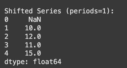

As you can see, the value at index 1 (12) is now 10 (the value from index 0). The value at index 2 (11) is now 12 (the value from index 1), and so on. This exactly replicates our “last known value” forecast, where shifted_series[t] is our forecast for data_series[t], based on data_series[t-1].

Implementing the One-Step-Ahead Forecast

Now, let’s apply this concept to our simulated random walk data, which we’ve been using in previous sections. We’ll assume the df DataFrame, containing our random walk, is already loaded and available.

import numpy as np
import pandas as pd
import matplotlib.pyplot as plt
from sklearn.metrics import mean_squared_error
# For demonstration, let's quickly re-create a simple random walk if df is not globally available
# In a real book, this would assume 'df' is carried over from previous sections.
np.random.seed(42) # for reproducibility
steps = np.random.normal(loc=0, scale=1, size=1000)
df = pd.DataFrame(100 + steps.cumsum(), columns=['value'])
# Generate the one-step-ahead forecast using the 'shift' method
# Each value in 'df_forecast' will be the previous value from 'df'
df_forecast = df.shift(periods=1)
# Display the first few rows of the original and forecasted DataFrame
print("Original DataFrame (first 5 rows):")
print(df.head())
print("\nForecasted DataFrame (first 5 rows):")
print(df_forecast.head())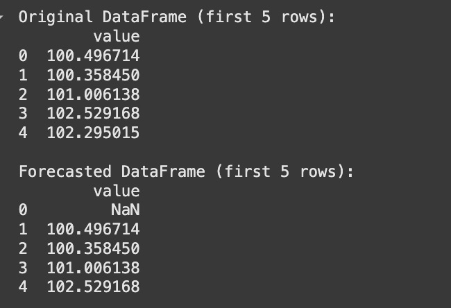

As expected, the first value of df_forecast is NaN, and subsequent values are simply the preceding values from df. This df_forecast now represents our one-step-ahead naive forecast.

Visualizing the Naive Forecast

Let’s visualize how this simple forecast performs against the actual random walk. You might be surprised by how “good” it looks.

# Create a figure and an axes object for the plot
fig, ax = plt.subplots(figsize=(12, 7))
# Plot the actual random walk values
ax.plot(df.index, df['value'], 'b-', label='Actual Values')
# Plot the one-step-ahead forecast
# We start from the second value as the first forecast is NaN, ensuring alignment
ax.plot(df_forecast.index, df_forecast['value'], 'r-.', label='One-Step-Ahead Naive Forecast')
# Add labels and title for clarity
ax.set_xlabel('Timestep')
ax.set_ylabel('Value')
ax.set_title('Random Walk: Actual vs. One-Step-Ahead Naive Forecast')
# Add a legend to distinguish the lines
ax.legend(loc='upper left')
# Ensure layout is tight to prevent labels from overlapping
plt.tight_layout()
plt.show()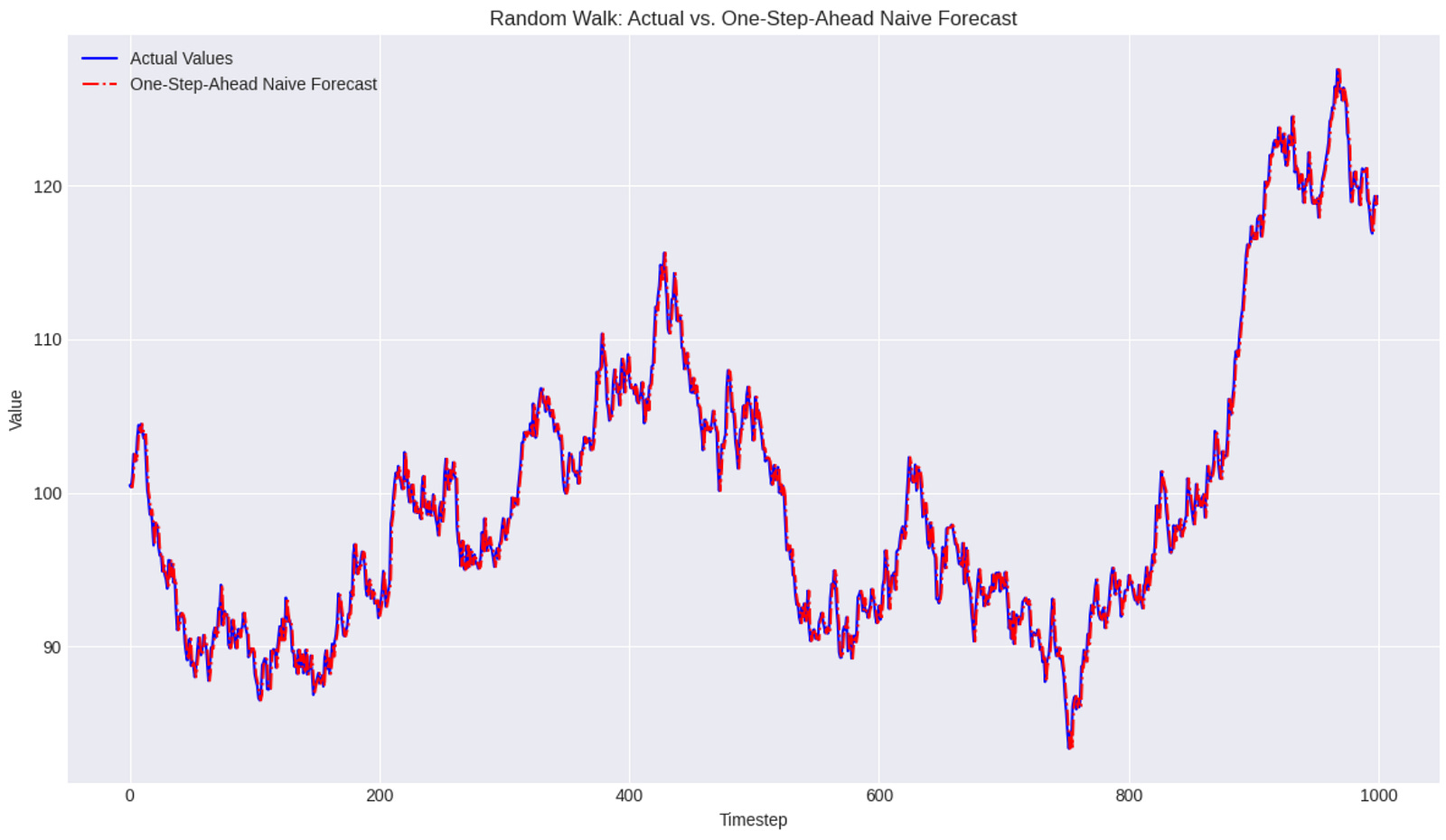

The plot strikingly shows the forecast line almost perfectly tracking the actual values, just slightly behind. This might lead one to believe that we’ve found a highly accurate predictive model for a random walk. However, this visual “perfection” is deceptive. It doesn’t signify true predictive power in the sense of anticipating future movements, but rather it’s a direct consequence of the random walk’s definition. Since Yt is essentially Yt − 1 plus some small, unpredictable noise, predicting Yt − 1 for Yt will naturally result in a very close fit, as the only difference is the unforecastable noise term.

Quantifying Performance with Mean Squared Error (MSE)

To quantitatively evaluate the forecast, we’ll use the Mean Squared Error (MSE). The MSE measures the average of the squares of the errors — that is, the average squared difference between the estimated values and the actual value. A lower MSE indicates a better fit.

When calculating MSE, it’s crucial to evaluate the model on unseen data. From previous sections, we typically split our data into a training set and a test set (e.g., the first 800 timesteps for training and the remaining 200 for testing). We will calculate the MSE on the test set portion of our data. Also, remember thatdf_forecast has a NaN at the first position, which needs to be handled by dropping NaNs before comparison.

# Define the start index for the test set, consistent with previous sections
test_start_index = 800
# Extract the actual values for the test set
test_actual = df['value'].iloc[test_start_index:]
# Extract the corresponding forecasted values for the test set
test_forecast = df_forecast['value'].iloc[test_start_index:]
# Create a combined DataFrame to easily drop rows where either actual or forecast is NaN
# This handles the initial NaN from the shift operation and ensures alignment
combined_data = pd.DataFrame({'actual': test_actual, 'forecast': test_forecast}).dropna()
# Extract the aligned actual and forecast values for MSE calculation
actual_for_mse = combined_data['actual']
forecast_for_mse = combined_data['forecast']
# Calculate the Mean Squared Error (MSE)
mse_one_step = mean_squared_error(actual_for_mse, forecast_for_mse)
print(f"Mean Squared Error (MSE) for one-step-ahead forecast on test set: {mse_one_step:.4f}")

Mean Squared Error (MSE) for one-step-ahead forecast on test set: 0.9304

The MSE value is approximately 0.93. This is a very low error, reinforcing the visual observation that the forecast is very close to the actual values.

Interpreting the MSE for a Random Walk

A low MSE for a random walk’s one-step-ahead forecast is not a sign of a powerful predictive model, but rather a direct reflection of the random walk’s underlying structure. The random walk equation is Yt = Yt − 1 + ϵt. When we forecast Yt as Yt − 1, our error is simply ϵt. Therefore, the Mean Squared Error of our forecast should theoretically be equal to the variance of the white noise term, Var(ϵt).

In our simulation, we generated the steps (which represent ϵt) using np.random.normal(loc=0, scale=1, size=1000), meaning the noise term has a mean of 0 and a standard deviation (and thus variance) of 1. Our calculated MSE of 0.9304 is very close to the expected variance of 1, confirming that our “forecast” is effectively just measuring the variance of the unpredictable noise component. It tells us nothing about predicting the direction or magnitude of future changes beyond the immediate past.

Practical Implications

This exercise highlights a critical lesson for time series analysis, especially in finance:

1. Fundamental Unpredictability: For processes that closely resemble random walks (like many financial asset prices), predicting future values beyond the very next step is practically impossible.

2. Naive Baselines are Powerful: The “last known value” forecast, despite its simplicity, serves as an excellent benchmark for random walk-like series. Any more complex model must significantly outperform this naive baseline to be considered truly valuable. Often, sophisticated models fail to beat this simple approach for random walks, especially over longer horizons.

3. Context is Key: A low error metric doesn’t always imply a “good” model in the traditional sense. For random walks, a low MSE for one-step-ahead forecasts merely confirms that the process behaves as a random walk, where the next value is largely determined by the current value plus random noise.

You are encouraged to experiment by changing the periods parameter in the shift() method. Observe how the visual fit deteriorates and the MSE increases rapidly as you try to forecast further into the future (e.g., periods=5, periods=10). This will visually and quantitatively reinforce the concept that random walks quickly become unpredictable beyond their immediate past.

Having thoroughly explored the nature and unique characteristics of random walks, it’s crucial to consolidate our understanding and establish a clear path forward for analyzing other types of time series. This section serves as a recap of the key takeaways regarding random walks and a bridge to more sophisticated modeling techniques applicable to series that exhibit different behaviors.

Understanding and Identifying Random Walks: A Recap

A random walk is a time series where the current value is simply the previous value plus a random shock. Mathematically, it can be expressed as Yt = Yt − 1 + ϵt, where ϵt is a white noise error term. This fundamental characteristic implies that the series has no memory of its past beyond the immediate prior step, and its future direction is entirely unpredictable.

Recalling the identification process is paramount, as correctly classifying a time series is the first step towards appropriate modeling. As previously illustrated (e.g., in Figure 3.20), identifying a random walk typically involves a multi-faceted approach:

Visual Inspection:

• Look for a non-constant mean (drift) or non-constant variance (heteroscedasticity). Random walks often exhibit apparent trends or shifts, but these are not true, deterministic trends; they are merely the accumulated effect of random steps.

• The series will not tend to revert to a mean.

Autocorrelation Function (ACF) and Partial Autocorrelation Function (PACF) Analysis:

• ACF: For a random walk, the ACF will decay very slowly, often linearly, remaining significantly positive for many lags. This slow decay is a hallmark of non-stationarity, indicating that past values have a persistent, but not necessarily predictive, influence on future values due to the cumulative nature of the random steps.

• PACF: The PACF of a random walk typically shows a single significant spike at lag 1 and then cuts off quickly or shows very small, insignificant spikes thereafter. This signifies that the direct dependence is only on the immediately preceding value.

Statistical Unit Root Tests:

• The Augmented Dickey-Fuller (ADF) test is the gold standard for statistically testing for the presence of a unit root, which is characteristic of a random walk. A unit root indicates that the series is non-stationary and that differencing is required to make it stationary. If the ADF test fails to reject the null hypothesis (that a unit root is present), it strongly suggests the series is a random walk.

Correctly performing these steps ensures that we do not mistakenly apply complex models to a series that is inherently unpredictable.

Forecasting Random Walks: Limitations and Best Practices

One of the most critical insights gained from studying random walks is their inherent unpredictability. Because each step is random and independent of previous steps (beyond the immediate last value), there is no underlying pattern or structure to exploit for forecasting.

Consequently, the most effective and statistically sound approach for forecasting a random walk is the naive forecast. This simply means that the best prediction for any future time step is the last observed value of the series.

• Forecasting the next timestep: For Yt + 1, the optimal forecast is Ŷt + 1 = Yt. Any attempt to use more sophisticated methods, such as averaging past values or fitting a linear model, will not yield better results and will likely introduce unnecessary complexity and potentially higher error.

• Forecasting on a long horizon: When forecasting multiple steps into the future, the naive forecast remains the last observed value: Ŷt + h = Yt for h > 0. However, the confidence intervals around this forecast will widen rapidly, reflecting the increasing uncertainty due to the accumulation of random shocks. This widening uncertainty underscores the practical limitation of forecasting random walks over longer periods — while the point forecast is flat, our confidence in it diminishes quickly.

The key takeaway is that for a random walk, advanced forecasting models are not just unnecessary; they are inappropriate. The best strategy is to acknowledge its unpredictability and rely on the simplest, most robust method.

Beyond Random Walks: Introducing Autoregressive (AR) and Moving Average (MA) Models

While random walks represent a fundamental type of time series, many real-world series do not behave in such an entirely unpredictable manner. Instead, they often exhibit stationarity (their statistical properties like mean, variance, and autocorrelation remain constant over time) but also possess autocorrelation (their past values influence their future values in a predictable, non-random way). For these series, more sophisticated models are not only appropriate but necessary to capture their underlying patterns and make accurate forecasts.

This is where Autoregressive (AR), Moving Average (MA), and combined Autoregressive Moving Average (ARMA) models come into play. These models are designed specifically to exploit the autocorrelation structure present in stationary time series.

Intuition Behind AR and MA Models

Autoregressive (AR) Models:

• Concept: An AR model predicts future values based on a linear combination of past values of the series itself. The “autoregressive” component implies that the series is regressed on its own past values.

• Intuition: Imagine a stock price that tends to move higher today if it moved higher yesterday. This suggests an autoregressive relationship. The model “remembers” its own past performance. An AR(p) model uses the previous p observations to predict the current value. For example, an AR(1)model suggests that the current value is directly dependent on the immediately preceding value plus a random error.

• Suitability: AR models are suitable for series where there’s a direct, measurable influence of previous observations on the current one.

Moving Average (MA) Models:

• Concept: An MA model predicts future values based on a linear combination of past forecast errors (or random shocks). It models the impact of past “noise” or “shocks” on the current value.

• Intuition: Consider a manufacturing process where a sudden, unexpected defect (a “shock”) today might have a lingering effect on production quality for the next few days, even after the initial cause is addressed. An MA model captures this kind of dependency. It’s not about the past value of the series directly, but about the impact of past unpredictable events. An MA(q) model uses the previous q forecast errors to predict the current value.

• Suitability: MA models are suitable for series where deviations from the mean (errors) in the past have a transient but predictable effect on current values. They are often useful for smoothing out short-term fluctuations caused by random disturbances.

Autoregressive Moving Average (ARMA) Models:

• Concept: An ARMA(p, q) model combines both AR(p) and MA(q) components. Many real-world time series exhibit both types of dependencies simultaneously.

• Intuition: An ARMA model provides a more comprehensive framework to capture the complex autocorrelation patterns found in many stationary series. It can model both the direct influence of past values and the lingering effects of past shocks.

The transition from random walks to AR, MA, and ARMA models marks a significant step in time series analysis. While random walks are inherently unpredictable, these advanced models provide powerful tools to analyze and forecast series that, though random to some extent, possess exploitable patterns within their statistical structure. The ability to correctly identify whether a series is a random walk or a stationary, autocorrelated process is fundamental, as it dictates the entire modeling strategy.

Summary: Unpacking Random Walks and Their Forecasting Frontier

This chapter has provided a deep dive into the fascinating, yet often counter-intuitive, world of random walks. Understanding random walks is fundamental in time series analysis, not only because they describe many real-world phenomena, particularly in finance, but also because they serve as a critical benchmark against which more complex models are evaluated. This section consolidates the key insights, reinforcing their definitions, identification methods, and, crucially, their unique forecasting implications.

Defining the Random Walk

A random walk is a time series where the current value is the sum of the previous value and a random shock. Mathematically, it can be expressed as:

Yt = Yt − 1 + ϵt

Where: * Yt is the value of the series at time t. * Yt − 1 is the value of the series at the previous time step t − 1. * ϵt is a random error term, often referred to as a “shock” or “innovation.”

The critical characteristic of the random shock ϵt is that it is typically assumed to be white noise. White noise is a series of independent and identically distributed (i.i.d.) random variables with a mean of zero and a constant variance. This means that each shock is entirely uncorrelated with previous shocks and has no predictable pattern.

This definition implies several key properties for a random walk: * Non-Stationary Mean: The mean of a random walk is not constant over time; it drifts. * Non-Stationary Variance: The variance of a random walk increases with time, meaning the uncertainty around future values grows as the forecast horizon extends. * Unpredictable Steps: Future steps are determined solely by the current position and a random, unpredictable shock. The past trajectory (beyond the immediate previous step) provides no information about the direction or magnitude of the next step.

Identifying Random Walks: The Quest for Stationarity

Identifying a random walk is paramount because it dictates the appropriate analytical and forecasting strategies. The core concept in this identification is stationarity.

Understanding Stationarity

A time series is considered stationary if its statistical properties — specifically its mean, variance, and autocorrelation structure — remain constant over time. This means that if you take any segment of a stationary series, its statistical characteristics will be similar to any other segment of the same length.

Visually, stationary series tend to fluctuate around a constant mean with a stable range of variation, exhibiting no obvious trends or increasing/decreasing volatility. In contrast, non-stationary series, like random walks, often display clear trends (upward or downward drifts) and/or changing variance (e.g., increasing volatility over time). Many traditional time series models rely on the assumption of stationarity for valid inference and forecasting.

The Augmented Dickey-Fuller (ADF) Test

The Augmented Dickey-Fuller (ADF) test is a formal statistical test used to determine if a time series has a unit root, which is a characteristic feature of non-stationary series like random walks.

• Null Hypothesis (H0): The time series has a unit root (i.e., it is non-stationary, like a random walk).

• Alternative Hypothesis (H1): The time series does not have a unit root (i.e., it is stationary).

When interpreting the ADF test results, we look at two main components: 1. Test Statistic: A more negative value suggests stronger evidence against the null hypothesis. 2. P-value: If the p-value is less than a chosen significance level (e.g., 0.05), we reject the null hypothesis and conclude the series is stationary. Conversely, a high p-value indicates that we fail to reject the null hypothesis, suggesting the presence of a unit root and non-stationarity.

For a random walk, the ADF test typically yields a high p-value, indicating non-stationarity.

Differencing for Stationarity

Since many time series models require stationarity, a common transformation technique for non-stationary series is differencing. Differencing involves calculating the difference between consecutive observations in a series.

The first difference of a series Yt is given by:

ΔYt = Yt − Yt − 1

For a random walk, taking the first difference yields:

ΔYt = (Yt − 1+ϵt) − Yt − 1 = ϵt

As we noted, ϵt is defined as white noise. This is a crucial insight: the first difference of a random walk is a white noise process. This property is a definitive characteristic of a random walk and is often confirmed by applying the ADF test to the differenced series, which should then show stationarity.

Logarithmic Transformations

While differencing addresses trends and unit roots, another common transformation is the logarithmic transformation. This is particularly useful when the variance of a time series increases with its level (heteroscedasticity).

The natural logarithm function compresses larger values more than smaller values. By taking the logarithm of a series, multiplicative changes (e.g., percentage changes) are converted into additive changes, which can help stabilize the variance and make the series more amenable to models that assume constant variance. For instance, if a stock price tends to fluctuate more wildly when its price is high, taking the logarithm can normalize these fluctuations across different price levels.

Autocorrelation Function (ACF)

The Autocorrelation Function (ACF) plot is a powerful visual tool for assessing the correlation of a time series with its own lagged values. It shows the correlation coefficients between Yt and Yt − k for various lags k.

For a random walk: * Original Series: The ACF plot of a random walk typically shows a very slow decay of autocorrelation, meaning that current values are highly correlated with past values, and this correlation persists over many lags. This slow decay is another strong indicator of non-stationarity and the presence of a unit root. * Differenced Series: After differencing, the ACF plot of a random walk’s first difference (ϵt) will resemble that of a white noise process. This means there will be a significant spike at lag 0 (correlation of a series with itself is 1) and then all other lags will be near zero, falling within the confidence bands. This confirms that all serial correlation has been removed, leaving only random noise.

Forecasting Random Walks: The Naive Approach

Perhaps the most critical takeaway from studying random walks is their profound implication for forecasting. Despite the sophistication of modern statistical models and deep learning architectures, these methods are generally ineffective for forecasting random walks beyond a single step.

Why Advanced Models Fail

The fundamental reason for this ineffectiveness lies in the definition of a random walk: each step is determined by the previous value plus a random, unpredictable shock. There is no underlying pattern, seasonality, or trend in the shocks that can be learned or extrapolated by complex algorithms. Any perceived patterns in a random walk are merely the result of accumulated random shocks, not inherent predictability. Training a sophisticated model on a random walk would be akin to trying to predict the outcome of a fair coin toss based on previous tosses — it’s inherently unpredictable.

The Power of Naive Forecasting

Given the inherent unpredictability of the random shock, the most statistically sound and practically effective method for forecasting a random walk is the naive forecast.

For a random walk, the best forecast for the next timestep (Yt + 1) is simply the last observed value (Yt):

Ŷt + 1 = Yt

This is because, on average, the expected value of the random shock ϵt + 1 is zero. Therefore, our best estimate for the next value is simply the current value, as we have no information to suggest it will move up or down beyond the current observation.

This principle extends to longer horizons: for any future timestep T > t, the best forecast for YT is still Yt. This highlights that for a random walk, forecasts beyond one step ahead provide no additional information and are no more accurate than simply using the last observed value. This was empirically demonstrated in our previous sections, showing that forecasting a random walk on a long horizon simply produces a flat line at the last observed value, with the confidence intervals widening dramatically, reflecting the increasing uncertainty.

In summary, random walks represent a benchmark of unpredictability in time series. Their non-stationary nature, identifiable through tools like the ADF test and ACF plots, necessitates transformations like differencing to achieve stationarity (revealing the underlying white noise). Most importantly, their inherent randomness dictates that naive, one-step-ahead forecasts are not just adequate, but often the optimal strategy, serving as a critical reminder that not all time series are predictable, and understanding these limitations is as crucial as mastering complex modeling techniques.