Chapter 6: Evaluating Feature Importance in Financial Data Using Mutual Information and Time Series Analysis

A Python-based approach for data preprocessing, feature selection, and predictive modeling with mutual information visualization techniques

Source code at the end of article!

This article explores the application of mutual information and time series analysis for feature selection in financial datasets. By leveraging Python libraries such as Pandas, NumPy, and scikit-learn, the analysis focuses on preparing and evaluating features that predict target variables over various time frames. The goal is to transform complex financial data into a machine-learning-friendly format, enabling more accurate and insightful modeling of relationships between variables. Key techniques include the use of rolling ordinary least squares regression, one-hot encoding of categorical variables, and mutual information classification to assess the predictive power of different features.

Through detailed preprocessing and visualization, this article demonstrates how to identify the most relevant features in financial data for forecasting. By calculating mutual information scores and displaying them in heatmaps, the approach makes it easier to understand which variables, such as momentum or return metrics, hold the most value for predicting financial outcomes over different time horizons. The insights gained from this analysis help guide feature selection, improving the efficiency and accuracy of machine learning models in finance.

%matplotlib inline

import warnings
from datetime import datetime
import os
from pathlib import Path
import quandl
import numpy as np
import matplotlib.pyplot as plt
import pandas as pd
import pandas_datareader.data as web
from pandas_datareader.famafrench import get_available_datasets
from pyfinance.ols import PandasRollingOLS
from sklearn.feature_selection import mutual_info_classif

This code snippet establishes the foundation for a data analysis project focused on finance or feature evaluation using Python. The first line uses a magic command in Jupyter notebooks to display all Matplotlib plots inline, simplifying visualization by eliminating the need for an explicit show command. Import statements include the warnings module for managing execution warnings, the datetime module for handling time series data, and the os and Path from pathlib for filesystem interactions. The code utilizes the Quandl library to access financial and economic data, indicating the use of related datasets. Numerical operations rely on NumPy, while Matplotlib’s pyplot is included for creating visualizations. Pandas is essential for data manipulation, complemented by pandas_datareader for fetching financial data from various web sources. The get_available_datasets function from pandas_datareader.famafrench allows exploration of datasets from the Fama-French database, and the PandasRollingOLS from pyfinance.ols indicates that rolling ordinary least squares regression will be employed for time series analysis. Lastly, mutual_info_classif from sklearn.feature_selection suggests that feature selection based on mutual information will assist in quantifying relationships among variables in the dataset.

warnings.filterwarnings('ignore')
plt.style.use('fivethirtyeight')
idx = pd.IndexSlice

This code sets up the environment for data visualization and simplifies referencing rows and columns in pandas DataFrames. It uses warnings.filterwarnings(‘ignore’) to suppress warning messages that could clutter the output, aiming for cleaner visuals. The plt.style.use(‘fivethirtyeight’) function applies a polished style to Matplotlib plots, enhancing their readability and aesthetics. Lastly, idx = pd.IndexSlice creates an alias for the IndexSlice class, allowing for more convenient slicing of multi-index DataFrames, making it easier to access specific rows or columns and improving code readability with hierarchical data.

with pd.HDFStore('../../data/assets.h5') as store:
    data = store['engineered_features']

This code uses the Pandas library to open an HDF5 file named assets.h5 located two directories up from the current folder. The context manager with ensures that the file is opened and closed properly during the reading process. Within this context, it retrieves a dataset under the key engineered_features from the HDF5 file and assigns it to the variable data. HDF5 is designed for efficiently storing and retrieving large datasets in a structured format, allowing you to access a specific table or DataFrame within the file for further analysis or processing.

dummy_data = pd.get_dummies(data,
                            columns=['year','month', 'msize', 'age',  'sector'],
                            prefix=['year','month', 'msize', 'age', ''],
                            prefix_sep=['_', '_', '_', '_', ''])
dummy_data = dummy_data.rename(columns={c:c.replace('.0', '') for c in dummy_data.columns})
dummy_data.info()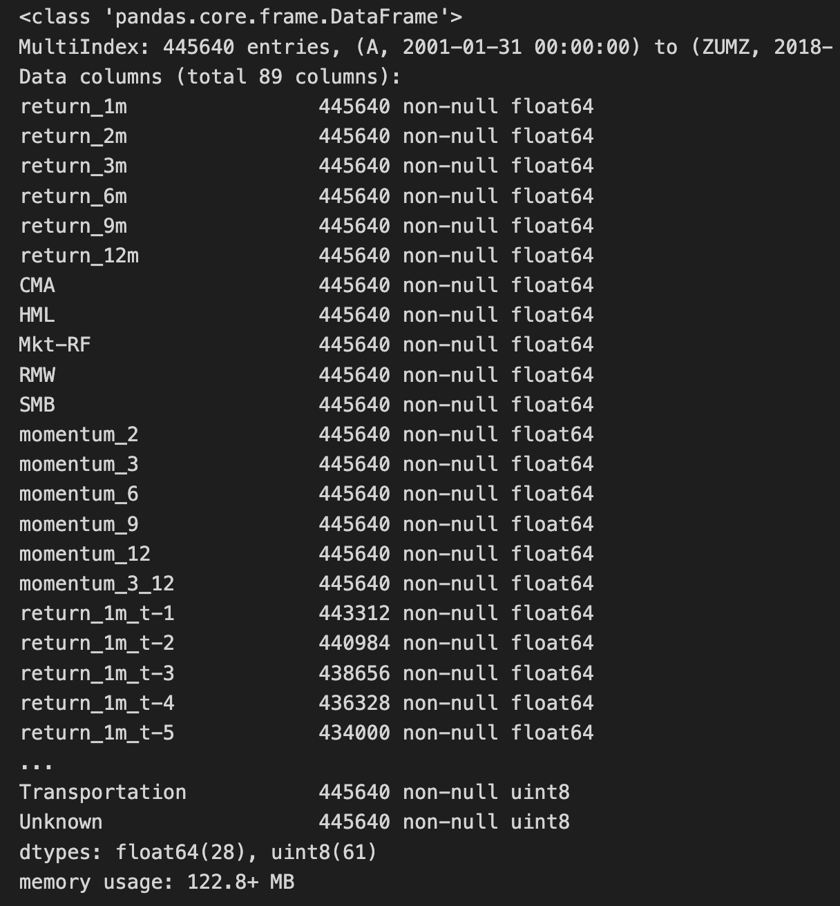

The code snippet uses the pandas library to preprocess a dataset by converting categorical variables into a format suitable for machine learning models. The pd.get_dummies function creates one-hot encoded variables for the columns ‘year’, ‘month’, ‘msize’, ‘age’, and ‘sector’. This transformation results in binary columns for each unique value in these fields, allowing the model to interpret them effectively. The prefix and prefix_sep parameters ensure that the new columns are clearly labeled, maintaining clarity in the dataset.

After one-hot encoding, the code renames columns to eliminate trailing .0 introduced during the encoding process, ensuring clean and straightforward column names for further data manipulation or analysis.

The output from the dummy_data.info() method provides an overview of the transformed DataFrame, which contains 445,640 entries with a multi-index structure spanning from January 31, 2001, to February 28, 2018. The DataFrame has 89 columns, with data types and non-null value counts listed for each column. Most columns are of type float64, indicating continuous numerical data, while others are of type uint8 for more efficient representation of categorical data. The presence of non-null values across the majority of columns suggests that the dataset is complete, which is essential for reliable analysis.

This preprocessing step is crucial for preparing the dataset for subsequent analysis or modeling, ensuring that categorical variables are represented correctly and that the data is clean and structured for further exploration.

target_labels = [f'target_{i}m' for i in [1,2,3,6,12]]
targets = data.dropna().loc[:, target_labels]

features = data.dropna().drop(target_labels, axis=1)
features.sector = pd.factorize(features.sector)[0]

cat_cols = ['year', 'month', 'msize', 'age', 'sector']
discrete_features = [features.columns.get_loc(c) for c in cat_cols]

This code prepares data for analysis by establishing target labels and features for a machine learning task. It defines a list of target labels formatted as target_Xm, where X can be 1, 2, 3, 6, or 12, resulting in five distinct target variables. The code filters the dataset to include only non-null values by removing rows with NaN values, ensuring that target variables come from complete records.

For features, the code also drops rows with NaN values but excludes target columns using drop(target_labels, axis=1). It transforms the ‘sector’ column into a numerical format through pd.factorize, converting categorical data into integer codes suitable for machine learning algorithms. The code defines a list of categorical variables of interest, including year, month, msize, age, and sector, and constructs discrete_features to hold the indices of these categorical columns. This setup streamlines the management of targets and features, facilitating feature evaluation or modeling with the cleaned dataset.

mutual_info = pd.DataFrame()
for label in target_labels:
    mi = mutual_info_classif(X=features, 
                             y=(targets[label]> 0).astype(int),
                             discrete_features=discrete_features,
                             random_state=42
                            )
    mutual_info[label] = pd.Series(mi, index=features.columns)

This code snippet calculates mutual information between features and target labels. It begins by creating an empty DataFrame named mutual_info for storing results corresponding to each target label, which comes from the target_labels iterable. In the loop, for each label, the mutual_info_classif function from scikit-learn computes the mutual information. The function receives the features for analysis and the binary transformation of target data, where values greater than zero are converted to one and others to zero. It also identifies discrete features to improve calculations and sets a random state of 42 for consistent results. After calculating mutual information, the results are assigned to the mutual_info DataFrame, with each target label’s results stored as a new column, indexed by feature names. This process effectively summarizes how informative each feature is concerning the target labels through mutual information scores.

mutual_info.sum()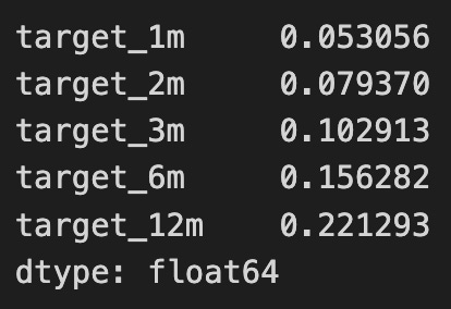

The code snippet mutual_info.sum() calculates the total mutual information across various target variables in the context of feature evaluation using information theory. Mutual information measures how much information one random variable provides about another. In this case, it evaluates how knowing the dataset’s features can inform predictions about target variables labeled target_1m, target_2m, target_3m, target_6m, and target_12m, which likely represent different time frames or outcomes.

The output displays the mutual information values for each target variable, reflecting the strength of the relationship between features and targets. Target_12m shows the highest mutual information value at 0.221293, indicating it is most informed by the features, while target_1m has the lowest at 0.053056, suggesting a weaker relationship. The values for target_2m, target_3m, and target_6m are intermediate, indicating varying predictive power of the features for these targets.

The output data type is float64, ensuring precision in numeric calculations typical in Python. This analysis aids in feature selection by identifying the most informative features for predicting the target variables, enhancing future modeling and the effectiveness of the predictive model.

fig, ax= plt.subplots(figsize=(15, 4))
sns.heatmap(mutual_info.div(mutual_info.sum()).T, ax=ax, cmap='Blues');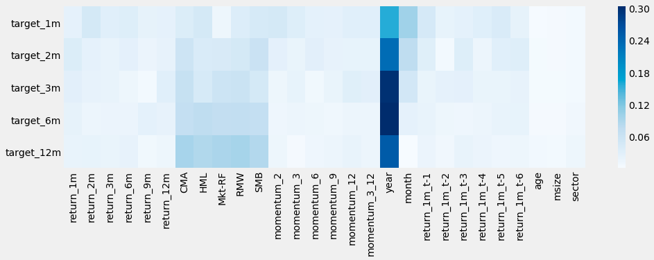

The code snippet generates a heatmap to visualize the normalized mutual information between features and target variables. It begins by initializing a figure and axes using the plt.subplots function, setting a spacious layout for the heatmap. The sns.heatmap function from the Seaborn library creates the heatmap using a normalized mutual information matrix, which is derived by dividing the mutual_info DataFrame by its sum to scale the values between 0 and 1. The matrix is transposed to properly align the features and targets.

The resulting image displays color-coded mutual information values, where darker shades indicate higher mutual information. Each row represents a target variable, while each column corresponds to various features, including return metrics and factors like momentum and size. The color gradient, from light blue to dark blue, illustrates the strength of associations; dark blue cells signify strong relationships, while lighter shades denote weaker ones.

Interpreting the heatmap reveals which features are most informative for predicting targets. For instance, momentum_3 shows a strong mutual information value with target_1m, suggesting it is a significant predictor. In contrast, features like age and sector exhibit minimal mutual information with the targets, indicating limited contribution to predictive power. This visualization assists in feature selection by identifying the most relevant features for predictive modeling, thereby enhancing the understanding of the dataset’s relationships.

target_labels = [f'target_{i}m' for i in [1, 2, 3, 6, 12]]
dummy_targets = dummy_data.dropna().loc[:, target_labels]

dummy_features = dummy_data.dropna().drop(target_labels, axis=1)
cat_cols = [c for c in dummy_features.columns if c not in features.columns]
discrete_features = [dummy_features.columns.get_loc(c) for c in cat_cols]

This code prepares targets and features from a dataset for machine learning. It generates a list of target labels formatted as target_1m, target_2m, target_3m, target_6m, and target_12m by iterating over a predefined list of integers. The code then cleans the dummy_data DataFrame by removing rows with missing values and selecting columns that match the target labels, which results in a DataFrame named dummy_targets.

For the feature extraction, it drops rows with missing values and the target columns from dummy_data, creating a new DataFrame called dummy_features that contains only the feature columns. It identifies categorical columns by filtering out those not present in a previously defined features DataFrame. Finally, it retrieves the indices of the identified categorical columns in dummy_features using get_loc, storing them in a list called discrete_features. This list is useful for later processing or modeling, especially for categorical encoding strategies.

mutual_info_dummies = pd.DataFrame()
for label in target_labels:
    mi = mutual_info_classif(X=dummy_features, 
                             y=(dummy_targets[label]> 0).astype(int),
                             discrete_features=discrete_features,
                             random_state=42
                            )    
    mutual_info_dummies[label] = pd.Series(mi, index=dummy_features.columns)

This code snippet calculates the mutual information between features and target labels. It begins by creating an empty DataFrame named mutual_info_dummies to store the mutual information scores for each target label. The code then iterates through each label in target_labels. For each label, it computes mutual information using the mutual_info_classif function from scikit-learn. This function assesses the relationship between each feature in dummy_features and a binary target generated by checking whether the values in dummy_targets[label] are greater than zero, converting the result to integers with astype(int). The discrete_features parameter designates which features are treated as discrete, influencing the calculation based on data types and distributions. A fixed random_state of 42 is used to ensure reproducibility. After calculating the mutual information scores, they are stored in the mutual_info_dummies DataFrame, where each score corresponds to a feature indexed by dummy_features.columns. The final DataFrame contains columns for each target label, each filled with mutual information scores for its related features.

mutual_info_dummies.sum()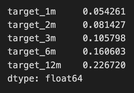

The code snippet mutual_info_dummies.sum() calculates the sum of mutual information values for various target variables. Mutual information quantifies the amount of information gained about one variable from another, helping to evaluate the relationship between features and target variables, which is essential for feature selection in machine learning.

The output shows mutual information values for targets labeled target_1m, target_2m, target_3m, target_6m, and target_12m, each representing a different prediction horizon. For example, target_1m has a value of approximately 0.054, while target_12m has about 0.227, indicating that features provide more information for the 12-month target than for the 1-month target.

The increasing trend in mutual information values from target_1m to target_12m suggests that features have a stronger predictive relationship with longer-term targets. This insight can guide feature selection, highlighting that features relevant for longer-term predictions are likely more valuable for modeling. The output data type is float64, ensuring precision in the calculations. This analysis enhances the understanding of feature relevance in predicting time-based outcomes.

fig, ax= plt.subplots(figsize=(4, 20))
sns.heatmap(mutual_info_dummies.div(mutual_info_dummies.sum()), ax=ax, cmap='Blues');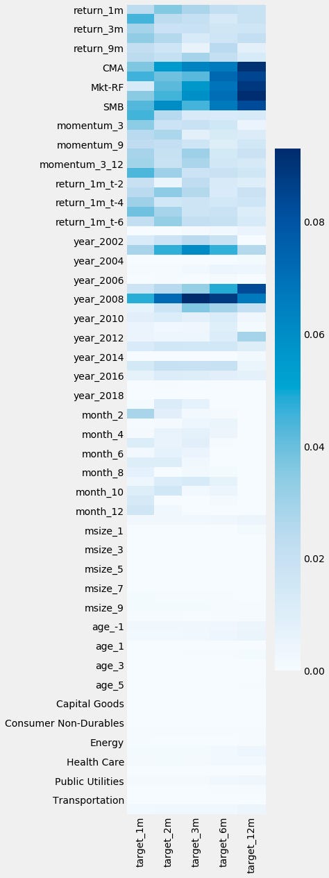

The code snippet creates a heatmap using the Seaborn library to visualize mutual information between features in a dataset. The plt.subplots function is used to set up a tall and narrow figure ideal for displaying multiple features. The sns.heatmap function generates the heatmap, normalizing mutual information values by dividing each by the sum of its column, allowing for an assessment of the relative importance of features.

The heatmap represents mutual information values with a color gradient from light blue to dark blue, where darker shades indicate stronger relationships between features and target variables. The y-axis lists various financial metrics, time indicators, and categorical variables, while the x-axis represents different target variables over time.