

Classification, Regression, and Clustering With Java
Previously, we discussed the most important Java libraries that are used to implement machine learning.

Classification, regression, and clustering are some of the basic machine-learning tasks we will examine in detail. There will be an introduction to basic algorithms for classification, regression, and clustering in each of the topics. Simple, small, and easily understood datasets will be used as examples.
This article will cover the following topics:
Data loading
Attribute filtering
Modeling classifications, regressions, and clusters
Model evaluation
Before you start
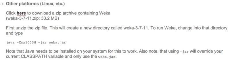
It is recommended that you download the most recent stable version of Weka from http://www.cs.waikato.ac.nz/ml/weka/downloading.html before starting.
You can download the file in multiple ways. Make sure you download the ZIP archive rather than the self-extracting executables since you will be using Weka as a library in your source code. You can find weka.jar within the extracted archive if you unzip the archive:
Follow these steps to show examples using the Eclipse IDE:
New Java project should be started.
Click on the Libraries tab and select Add External JARs after right-clicking on the project properties.
Click on the weka.jar file to extract the Weka archive.
The basics of machine learning are now ready for implementation!
The classification system
As a starting point, let’s take a look at how classification is commonly used in machine learning. According to the first article in this series, the main goal is to automatically map input variables to outcomes. Following are sections on loading data, selecting features, implementing a basic classifier in Weka, and evaluating it.
Data
The ZOO database is the resource we will use for this task. As shown in the following table, the database contains 101 records describing animals with 18 attributes:
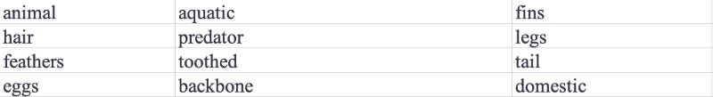
This dataset shows an example of a lion, which has the following attributes:
animal: lion
hair: true
feathers: false
eggs: false
milk: true
airborne: false
aquatic: false
predator: true
toothed: true
backbone: true
breathes: true
venomous: false
fins: false
legs: 4
tail: true
domestic: false
catsize: true
type: mammal
Using all the other attributes as inputs, we will build a model to predict the outcome variable, animal.
The data is being loaded
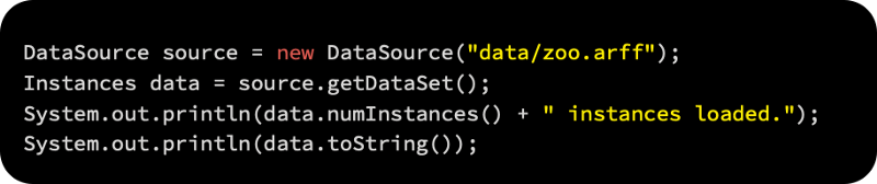
As a first step, Weka’s Attribute-Relation File Format (ARFF) is used to load the data and display the total number of loaded instances. A DataSource object contains each sample of data, while an Instances object contains the whole dataset, along with meta-information.
A DataSource object will be used to load the input data, which converts the files to Instances.
As an output, this will give you the number of loaded instances as follows:
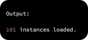
A complete dataset can also be printed by calling data.toString().
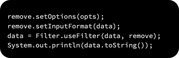
In the future, we will have to learn a model that can predict the animal attribute without knowing the animal label, based on other attributes. Therefore, the animal attribute will be removed from the training set. The Remove() filter will be used to remove the animal attribute.
In order to remove the first attribute, we first set a string table of parameters. For training a classifier, we use the remaining attributes:
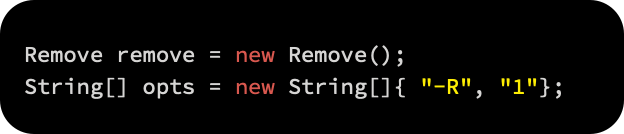
After that, we call the static method Filter.useFilter(Instances, Filter) to apply the filter to the selected dataset:
Feature selection
A preprocessing step called feature selection, also known as attribute selection, is discussed in the article Applied Machine Learning Quick Start. A learned model is created by selecting a subset of relevant attributes. What are the advantages of feature selection? Models are easier to interpret when they have a smaller set of attributes. As a result, overfitting is reduced and training time is usually shortened.
A class value can be taken into account when selecting attributes or it cannot. The first case is a selection algorithm that calculates a quality score for each selected attribute by evaluating each subset of features. In addition to extensive and best-first searches, we can use other search algorithms and quality scores, such as information gain and Gini coefficients.
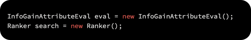
An AttributeSelection object supports this process, which requires two additional parameters: an evaluator to determine how informative an attribute is, and a ranker to sort attributes based on the evaluator’s score.
The following steps will guide us through the selection process:
Our evaluator in this example will be information gain, and the features will be ranked by information gain:
AttributeSelection will be initialized with the evaluator, ranker, and data as follows:
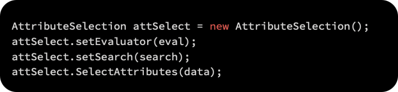
The order of attribute indices will be printed as follows:
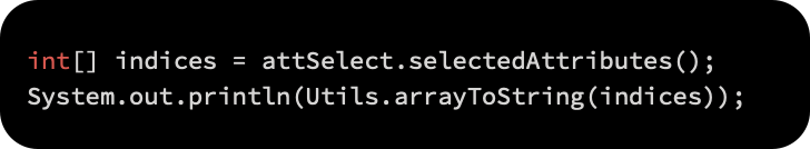
As a result of this process, the following result will be produced:
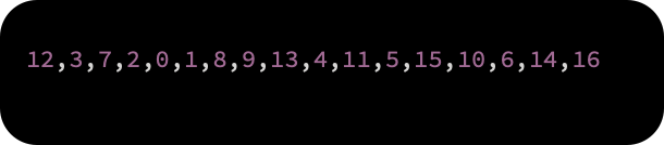
Twelve (fins), three (eggs), seven (aquatic), two (hair), and so on are the most informative attributes. In this way, we can help learning algorithms achieve more accurate and faster learning models by removing additional, non-informative features.
If we were to keep a certain number of attributes, how would we decide? Data and the problem determine the number of attributes; there is no set rule of thumb. In selecting attributes, you should consider whether the attributes improve your model rather than whether they serve the model better.
Learning algorithms
Data has been loaded and features have been selected, and we are now ready to learn some classification models. The first step is to understand the basics of decision trees.
Quinlan’s famous C4.5 decision tree learner (Quinlan, 1993) is reimplemented in Weka’s J48 class.
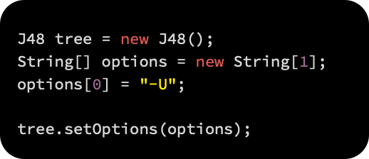
Using the following steps, we will create a decision tree:
The J48 decision tree learner is initialized. String tables can be used to pass additional parameters, such as tree pruning that controls the complexity of the model. Due to the fact that we are building an unpruned tree, we will only pass the -U parameter:
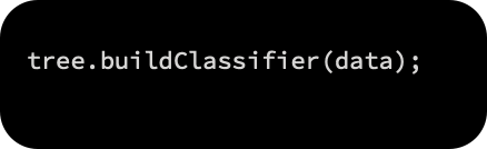
The learning process is initiated by calling the buildClassifier(Instances) method:
A tree object is now used to store the built model. To provide the unpruned J48 tree, we can use the toString() method:
As a result, we will get the following:
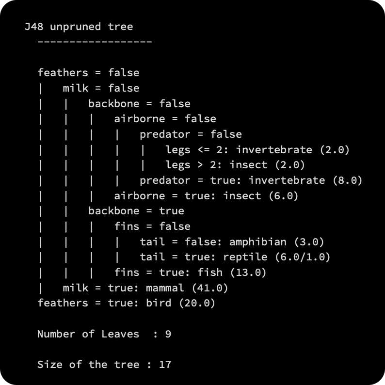
Nine of the 17 nodes in the output tree are terminal (leaves).
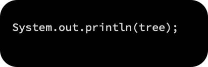
Alternatively, you can use the TreeVisualizer tree viewer to display the tree, as follows:
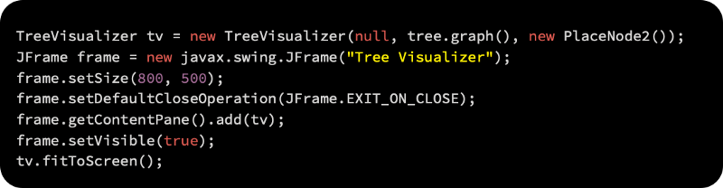
In the following output frame, the preceding code is executed:
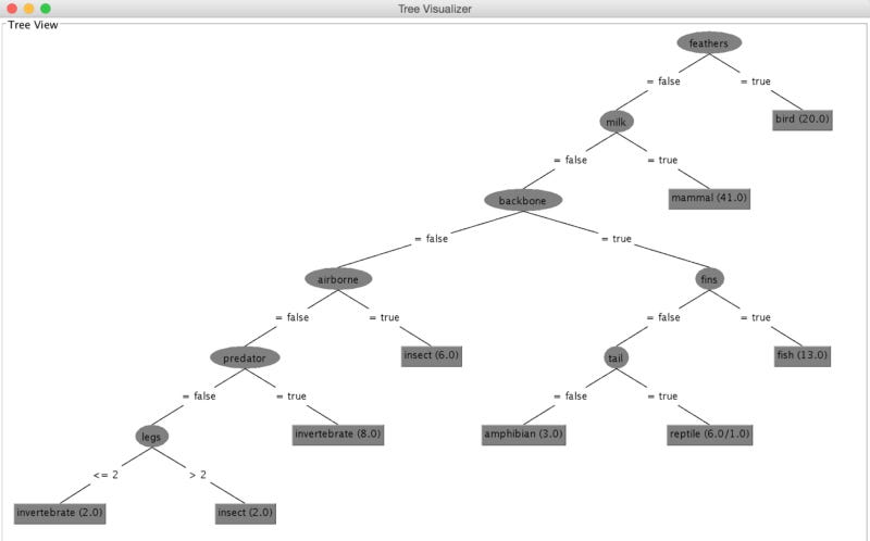
Top nodes, also called root nodes, are the starting point of the decision process. An attribute value is specified by the node label. The feathers attribute is checked first in our example. Following the right branch leads to the leaf labeled bird, which indicates 20 examples support this conclusion if the feather is present. The left-hand branch is followed if there is no feather, which leads us to the milk attribute. Following the branch that matches the attribute value, we check the value of the attribute once again. The process is repeated until a leaf node is reached.
In the same fashion, we can construct other classifiers by passing the parameters determining the model complexity to the buildClassifier(Instances) method.
In the next section, you will learn how to assign an unknown class label to a new example using a trained model.
Data classification
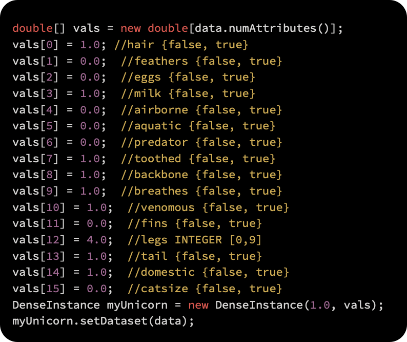
The learned classification model can be used to predict the label of an unknown animal whose attributes have been recorded. For this process, we will use the following animal:

In order to describe the new specimen in more detail, we first construct a feature vector:
The model’s class value is obtained by calling classify(Instance). As a result of the method, the label index is returned as follows:
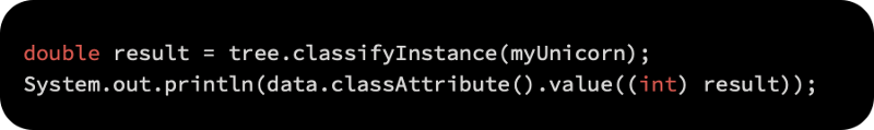
A mammal class label will be provided as an output.
Metrics for evaluating and predicting error
A model was built, but we don’t know whether it can be trusted. By applying a cross-validation technique, we can estimate its performance.
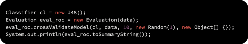
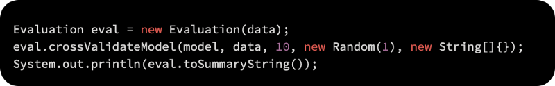
For implementing cross-validation, Weka provides an Evaluation class. Here is how we pass the model, the data, the number of folds, and a random seed:
The Evaluation object stores the results of the evaluation.
The toString() method provides a mix of metrics that are commonly used. It is important to pay attention to the metrics that make sense, since the output does not differentiate regression and classification:
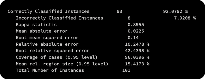
The number of instances that are correctly classified or incorrectly classified is important in the classification.
Matrix of confusion
We can also examine the confusion matrix to determine where a particular misclassification has occurred. An example of how a specific class value was predicted is shown in the confusion matrix:
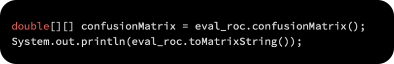
Following is the confusion matrix:
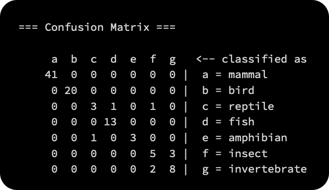
A classification node assigns labels to the columns in the first row. A true class value is then assigned to each additional row. The second row, for instance, corresponds to instances with the mammal true class label. As we can see in the column line, all mammals were correctly classified as mammals. Three of the reptiles in the fourth row were correctly classified as reptiles, while one was classified as fish and one as insect. It enables us to understand the types of errors that can be made by our classification model through the confusion matrix.
Choosing an algorithm for classification
Naive Bayes is an inductive algorithm that is simple, efficient, and effective. Even with dependent features, its performance is amazingly competitive, even when features are independent, which is seldom the case in the real world (Zhang, 2004). Its main disadvantage is that it cannot learn how features interact with each other. For example, even if you like lemon and milk in your tea, you hate it when both are in it simultaneously.
We studied in our example that the decision tree is an easy-to-understand and easy-to-explain model. You don’t have to worry about linear separability of the data when you use it, since it can handle both nominal and numeric features.
In addition, the following algorithms can also be used for classification:
In addition, if your classifier’s performance is worse than the average value predictor, it is not worth considering this rule. Weka.classifiers.rules.ZeroR: This predicts the majority class and is considered a baseline.
In weka.classifiers.trees.RandomTree, K randomly chosen attributes are considered at each node of the tree.
The RandomForest class constructs a set (forest) of random trees and uses majority voting to classify new instances.
Based on cross-validation, this k-nearest neighbor classifier is capable of selecting the appropriate number of neighbors.
Using backpropagation, weka.classifiers.functions.MultilayerPerceptron is a classifier based on neural networks. It is possible to build a network manually or using an algorithm.
Based on the analysis of the training data, weka.classifiers.bayes.NaiveBayes uses numeric estimator precision values to create a Naive Bayes classifier.
The AdaBoost M1 method is used to boost a nominal class classifier in weka.classifiers.meta.AdaBoostM1. It is possible to tackle only nominal class problems. Often, this leads to dramatic improvements in performance, however, it can also result in overfitting.
A classifier can be bagged to reduce its variance by using weka.classifiers.meta.Bagging. In addition to classification, it can also perform regression, depending on the base learner.
Using Encog to classify
You learned how to use the Weka library for classification in the previous section. The purpose of this section is to quickly show how the Encog library can achieve the same thing. In order to classify using Encog, we must build a model. Visit https://github.com/encog/encog-java-core/releases to download the Encog library. The .jar file must be added to the Eclipse project once it has been downloaded, as explained at the beginning of the article.
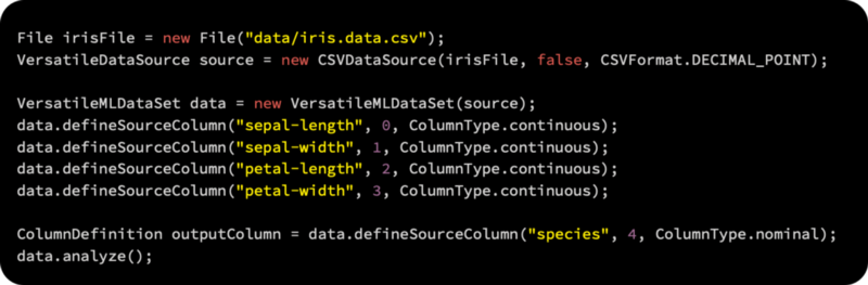
The iris dataset is available as a .csv file from http://archive.ics.uci.edu/ml/datasets/Iris and can be downloaded from there. In your data directory, copy iris.data.csv from the download path. A file containing 150 different flower data can be found here. Among the four columns are measurements and labels related to the flowers.
The following steps will be used to classify the data:
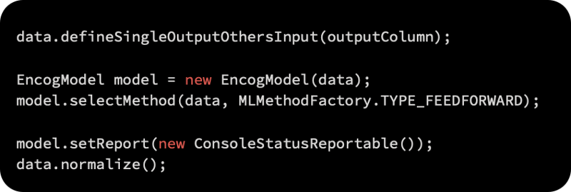
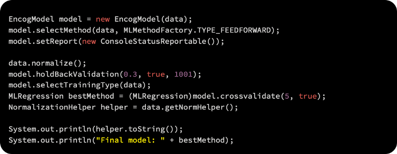
All four columns will be defined using the VersatileMLDataSet method. Using the analysis method, we can find the statistical parameters in the file, such as mean, variance, and standard deviation:
Defining the output column is the next step. Once the data has been normalized, it’s time to select the model type according to which the data will be normalized, as follows:
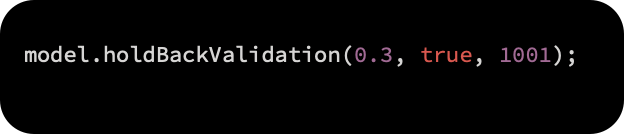
As the next step, a training set is used to fit the model, leaving a test set aside. According to the first argument, 0.3, we will hold 30% of the data; the next argument specifies to shuffle the data randomly. A holdback validation model is used because 1001 says there is a seed value of 1001.
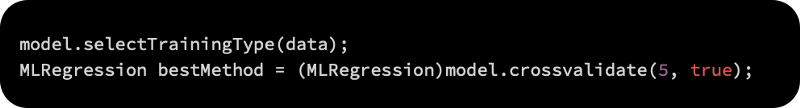
The model needs to be trained and the data categorized according to measurements and labels. Five different combinations of the training dataset are used for cross-validation:
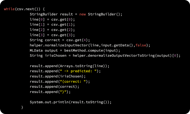
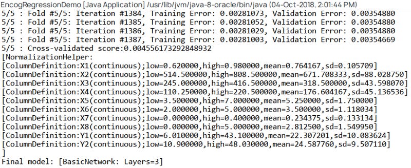
In the next step, we will display the results and errors of each fold:

Using the following code block, we will predict the values using the model:
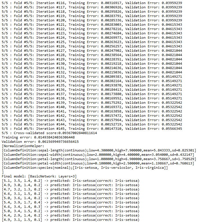
As a result, you will get the following output:
In addition to SVM and PNN, Encog supports many other methods in MLMethodFactory.
An evaluation
Following the development of the model, evaluation is the next important step. By comparing the model’s output to the dataset, you can determine whether it is performing well and whether it will be able to handle data it has never seen before. Following are the main features of the evaluation framework:
Error estimation: In this method, holdouts or interleaved tests and trains are used to estimate the errors. The data is also cross-validated using a K-fold method.
A more sensitive performance metric is Kappa, which is used to measure stream classification.
Comparing and evaluating classifiers requires comparing random and non-random experiments. For determining the statistical significance of differences between two classifiers, McNemar’s test is the most popular test in streaming. We can determine the reliability of a classifier based on the confidence intervals of parameter estimates.
In order to evaluate the process, we look at the cost per hour of usage and memory as we are dealing with streaming data that may require access to third-party or cloud-based solutions for access and processing.
Baseline classifiers
In addition to divide-and-conquer classifiers, lazy learners, kernel methods, graphics models, and so on, batch learning has contributed to the development of many other classifiers as well. Streaming the same data has the advantage of being incremental and fast, so we need to understand how to handle large datasets in streams. Model complexity must be weighed against model update speed, and this is the main trade-off to be considered.
Most classifiers are based on the majority class algorithm, which is used as a baseline. Decision tree leaves are also classified using this classifier. An alternative classifier predicts new instances’ labels based on no-change classifiers. A simple and low-cost method for calculating probabilities, Naive Bayes offers both. The algorithm is incremental and is best suited to streams.
Decision tree
In addition to being easy to interpret and visualize, decision trees are a very popular classifier technique. Trees are used in it. The leaves of the tree usually belong to the majority class classifier as it divides or splits the nodes based on their attribute values. This is a very fast decision tree algorithm for streaming data; instead of reusing instances, Hoeffding trees wait for new instances. For large data sets, a tree is built.
It maintains a model consistent with the instances in a sliding window through a concept-adapting Very Fast Decision Tree (CVFDT). In addition to the UFFT, there is the Hoeffding adaptive tree, the exhaustive binary tree, and so on.
Lazy learning
It is the most convenient batch method for streaming data to use k-nearest neighbor (KNN). When a new instance is not yet classified, the KNN is determined using a sliding window. The sliding window normally uses 1,000 instances from the most recent 1,000 observations. Concept drift is also handled by the sliding window as it slides.
Active learning
Stream data is not always classifiable by classifiers when compared with labeled data. Unlabeled data may be found in a stream, for instance. Unlabeled data must be labeled manually, which is costly. Data generated by streams is large. Only selective data is labeled by active learning algorithms. In a pool-based setting, historical data is used to label the data. It is necessary to retrain the system periodically in order to determine whether an incoming instance needs a label. A random strategy can be used to label data simply. In this method, a label is requested for every incoming instance with a probability of a budget for labeling. The least confident instance may also be asked for a label. Until the classifier reaches its threshold or exhausts its budget, this method may work well.
Regression
Using a dataset on energy efficiency, we will examine basic regression algorithms. According to their construction characteristics, such as their surface, wall, and roof areas, heights, glazing areas, and compactness, we will calculate the heating and cooling load requirements for the buildings. By varying 18 building characteristics, the researchers designed 12 different house configurations. Simulated buildings totaled 768.
A systematic analysis of each building characteristic’s impact on the target variable, that is, the heating or cooling load, is our first objective. Another goal is to compare a linear regression model with other approaches, such as a SVM regression, a random forest, or a neural network. Using the Weka library, we will accomplish this task.
Loading the data
The data on energy efficiency can be downloaded from https://archive.ics.uci.edu/ml/datasets/Energy+efficiency.
There are XLSX files in the dataset that Weka cannot read. The following screenshot shows how we can save it as a comma-separated value (CSV) file by clicking File | Save As and selecting .csv. If you choose to save only the active sheet (since all the other sheets are blank), you may lose some formatting features. The file is now ready for Weka to load:

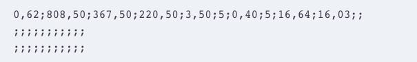
Make sure the file was transformed correctly by opening it in a text editor. There may be some minor issues that need to be addressed. A double semicolon ended each line of my export, for example:
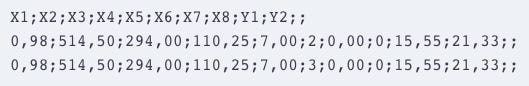
By using the Find and Replace function, you can remove the doubled semicolon: find ;; and replace it with ;.
As for the second problem, I had a long list of empty lines at the end of the document, which I can delete by following these steps:
Now that the data has been loaded, we can begin working with it. The following code will demonstrate how to import CSV files using Weka’s converter for reading CSV files:
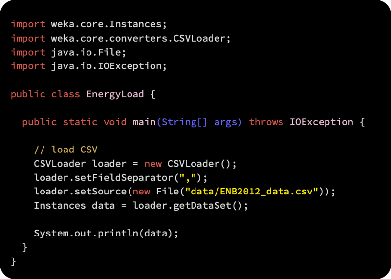
We have loaded the data! It’s time to move on.
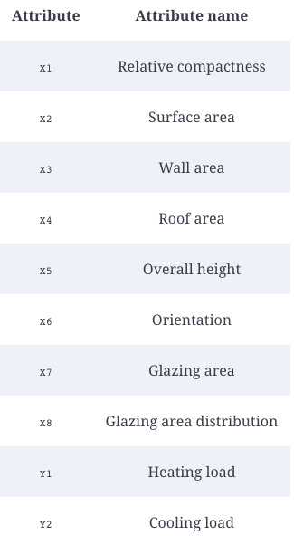
Attribute analysis
The first thing we should do is understand what we are dealing with before analyzing the attributes. As shown in the following table, there are eight attributes that describe the building characteristics, as well as two target variables:
Regression model construction and evaluation
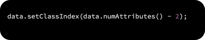
The class attribute is set at the feature position in order to start learning a model for heating load:
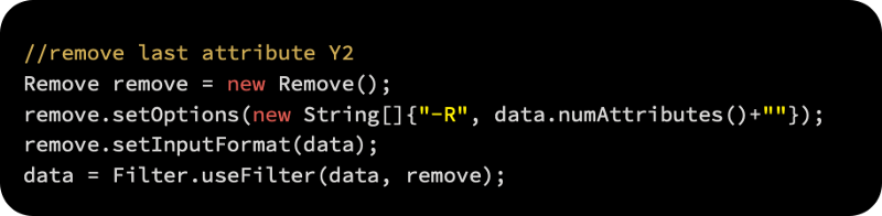
We can now remove the cooling load variable from the second target variable:
Linear regression
With the LinearRegression class, we will implement a simple linear regression model.
Our approach will be similar to that used in the classification example by creating a new model instance, passing the parameters and data, and then calling buildClassifier(Instances):
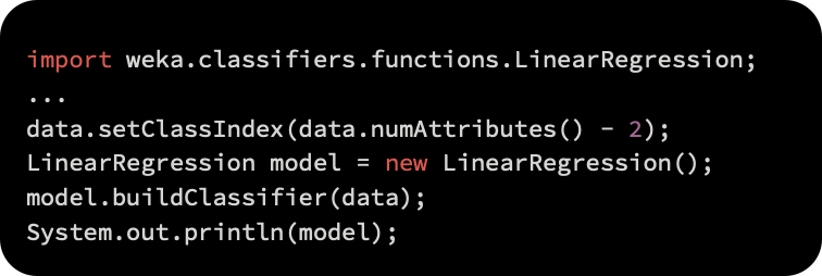
The buildClassifier(Instances) method will be invoked following the same procedure as in the classification example
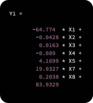
By combining the input variables linearly, the linear regression model estimates the heating load. In addition to the sign and magnitude, the number in front of the feature describes how the feature affects the target variable. A negative correlation exists between the relative compactness of feature X1 and the heating load, while a positive correlation exists between the glazing area and the heating load. The final estimate of the heating load is also affected by these two factors. By using cross-validation, the performance of the model can also be evaluated.
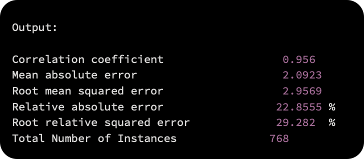
As a result of the ten-fold cross-validation, the following results were obtained:
A number of common evaluation metrics, including correlation, mean absolute error, relative absolute error, etc., can be generated, as follows:
Encog-based linear regression
We will now examine how Encog can be used to make a regression model. In this section, we will use the dataset that we loaded in the previous section. Making the model can be done in the following steps:
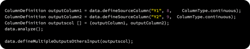
We will load the data using the VersatileMLDataSet function as follows:
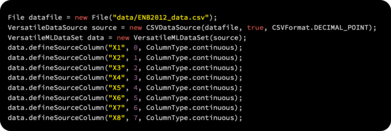
The defineMultipleOutputsOthersInput function can be used to add the two outputs, Y1 and Y2, as follows:
Using FEEDFORWARD, we build a simple regression model:
Now we have a regression model ready to use. As shown in the screenshot below, the last few lines of the output are as follows:
Trees of regression
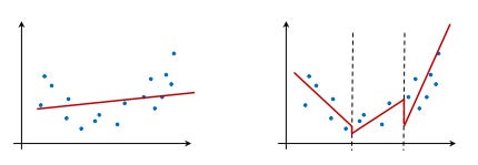
Alternatively, the data can be analyzed using a set of regression models, each using its own part of the data. Regression models and regression trees are illustrated in the following diagram. Regression models construct one model that fits all the data best. However, regression trees construct a set of regression models, each modeling a part of the data, as shown on the right. Regression trees can better fit data than regression models, but the function is piece-wise linear, with jumps between modeled regions, as shown below:
Within the M5 class, Weka implements a regression tree. As with any model, the method buildClassifier(Instances) should be invoked once the model has been initialized, the data and parameters passed, and the model’s parameters passed:
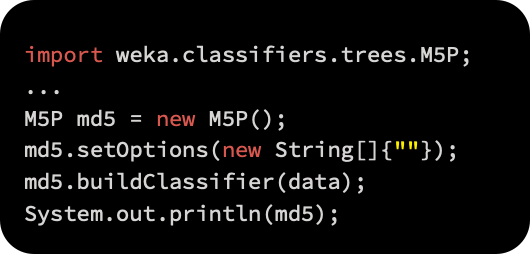
There are equations in the leaf nodes of the induced model, as follows: