

Containerized Quant: Forecasting Markets with ML
A step-by-step guide to building a robust stock prediction engine from scratch.

Download the source code using the button at the end of this article!
Building a profitable algorithmic trading strategy takes more than just a clever neural network; it requires rock-solid engineering plumbing. Too many tutorials focus purely on the machine learning model, leaving you to figure out how to ingest raw market data, align technical indicators, and manage the deadly trap of temporal data leakage. Alright, we’re going to change that. In this guide, we aren’t just training a model — we are architecting a complete, containerized system.
Together, we will build an end-to-end machine learning pipeline from scratch. We’ll start by hooking into the Alpha Vantage API to systematically fetch daily stock prices and technical indicators, merging them into a clean, time-aligned dataset. From there, we’ll construct a bulletproof preprocessing stage that handles missing data, scales features without looking into the future, and prepares our sequences for supervised learning. Finally, we’ll train and evaluate a TensorFlow neural network to forecast the next trading day’s adjusted close.
By the end of this walkthrough, you won’t just have a theoretical script running on your local machine. You will have a portable, Docker-backed trading architecture that handles the entire lifecycle: fetch, preprocess, train, and evaluate. Whether you want to stick with the baseline feedforward network or eventually upgrade to a time-series model like an LSTM, you’ll have the exact infrastructure needed to test your quantitative strategies with confidence.
# file path: run.sh
docker run -it --rm --name my-running-app stock-prediction
run.sh serves as the runtime trigger for the entire pipeline by launching the Docker image named stock-prediction as a container instance; it creates a container with the name my-running-app, attaches an interactive terminal to it so you can see logs and interact if needed, and ensures the container is removed automatically when it exits. In the project flow, run.sh is the simple handoff from local environment into the packaged runtime: build.sh is the companion script that produces the stock-prediction image by building the application, while the Python entrypoint inside the image is the code that actually imports and sequences fetch_combined_data, preprocess, neural_network, and evaluate_neural_network to perform fetch → preprocess → train → evaluate. run.sh does not perform those stages itself; it just starts the container whose default entrypoint executes the end-to-end orchestration described by the imports.
# file path: build.sh
docker build -t stock-prediction .
build.sh is the tiny convenience script that produces a portable runtime for the pipeline by invoking Docker to build an image for the project; it takes the repository’s Dockerfile and produces an image tagged stock-prediction that encapsulates the environment and all dependencies the training/evaluation flow needs. In the context of the staged ML pipeline, its role is to create the reproducible execution artifact that later steps will run: the image it builds contains the code that fetches historical JSONs, runs preprocessing, trains the per-symbol TensorFlow models, and produces evaluation artifacts so the pipeline can be executed identically across machines. There is no branching or data processing in build.sh itself—its single responsibility is image creation—so it sits standalone in the repo and is not invoked by other Python modules. build.sh pairs directly with run.sh, where run.sh starts a container from the image built here and provides the interactive runtime semantics (for example, creating and removing a running container), whereas the project’s Python import statements in other modules are unrelated to this script and live inside the image that build.sh produces.
# file path: scripts/constants.py
BASEURL = ‘https://www.alphavantage.co/query?’
BASEURL defines the root HTTP endpoint used across the pipeline to request market data from Alpha Vantage; during the fetch stage the code composes full request URLs by appending function, symbol, interval, API key and other query parameters to this base so the pipeline can retrieve the historical price and indicator JSONs it needs for preprocessing. As a project-wide constant it centralizes the remote service address so fetch logic imports a single source of truth rather than hard-coding the domain in multiple places; the value intentionally includes the query-string separator to make simple concatenation of parameters straightforward. You will see BASEURL combined with API_KEY when authenticating requests and with TIME_SERIES_DAILY_ADJUSTED and INTERVAL when selecting the specific time-series function and granularity for the next-day adjusted-close data the pipeline ingests.
# file path: scripts/constants.py
API_KEY = ‘NHX8KHJFCBEJFJ7P’
API_KEY is the module-level constant that stores the Alpha Vantage credential the fetch step uses to authenticate outbound market-data requests; during a pipeline run the fetcher reads API_KEY alongside BASEURL to construct the HTTP query that retrieves historical price and indicator JSONs, and those responses then flow into the preprocessing stage. It follows the same pattern as other constants like BASEURL, INTERVAL, and TIME_SERIES_DAILY_ADJUSTED by centralizing a fixed configuration value here so every part of the codebase uses a single source of truth for API parameters and avoids scattering hard-coded strings.
# file path: scripts/constants.py
INTERVAL = ‘daily’
INTERVAL is the global configuration constant that tells the pipeline which sampling frequency to treat the market data as — in this project it is set to a daily cadence so every fetch, gap-fill, label construction, sequence splitting, and model step is aligned to one trading-day resolution. In practice the fetch step uses INTERVAL to decide which time bucket to request from the market/indicator feeds, the preprocessing stage uses it to infer the expected spacing when filling missing dates and resampling, and the supervised-label logic uses it to define the prediction horizon (next-day adjusted-close is meaningful because the interval is daily). This is complementary to TIME_SERIES_DAILY_ADJUSTED, which names the specific API time-series endpoint the code will call; INTERVAL expresses the temporal granularity the pipeline consumes, whereas TIME_SERIES_DAILY_ADJUSTED is the API method that supplies that granularity. By contrast TIME_PERIOD is a numeric window size used for indicator calculations and looks like a different kind of configuration (a count of past steps rather than a temporal label), and API_KEY holds the credential for the external data service; INTERVAL is about frequency, TIME_PERIOD is about window length, and API_KEY is about authentication.
# file path: scripts/constants.py
TIME_PERIOD = ‘10’
TIME_PERIOD holds the project-wide setting that defines how many past time steps the preprocessing and modeling stages consider when building features and supervised sequences — in other words it specifies the lookback window used to compute rolling indicators, assemble input sequences for the TensorFlow models, and align labels for next-day adjusted-close forecasting. It is expressed as a string to remain consistent with other configuration entries such as INTERVAL, TIME_SERIES_DAILY_ADJUSTED, and OUTPUTSIZE_FULL so the same constant can be passed straight into routines and API callers that expect textual parameters; INTERVAL controls sampling frequency, TIME_SERIES_DAILY_ADJUSTED names the API payload key for the data source, and OUTPUTSIZE_FULL dictates how much history is fetched, while TIME_PERIOD determines how many of those fetched points will be combined into each training example.
This Substack is reader-supported. To receive new posts and support my work, consider becoming a free or paid subscriber.
# file path: scripts/constants.py
SERIES_TYPE = ‘close’
SERIES_TYPE declares which price series the pipeline will treat as the primary numeric series to extract from incoming market feeds and to use through preprocessing, model input construction, and target-label creation; in this configuration it selects the close price series. During the fetch stage the pipeline composes API requests using BASEURL and the function name held in TIME_SERIES_DAILY_ADJUSTED (with the temporal granularity controlled by INTERVAL) and then pulls the named series out of the returned JSON by matching the key indicated by SERIES_TYPE, converting those values into the time-indexed arrays that the preprocessing stage fills, scales, and converts into supervised examples for training and evaluation. As a project-wide constant, SERIES_TYPE centralizes that choice so every script references the same price field rather than hard-coding different keys in multiple places.
# file path: scripts/constants.py
TIME_SERIES_DAILY_ADJUSTED = ‘TIME_SERIES_DAILY_ADJUSTED’
TIME_SERIES_DAILY_ADJUSTED is the module-level constant that names the top-level key Alpha Vantage uses to return the daily adjusted time-series block in its JSON responses; the fetch stage uses that constant to locate the nested dictionary of date-indexed price records so the preprocessing stage can turn those per-day entries into a clean series for labeling, scaling, and sequence-splitting. This plays the same centralization role as INTERVAL, BASEURL, and SERIES_TYPE in the constants file—INTERVAL holds the request granularity used when composing API calls, BASEURL is the endpoint used to fetch data, and SERIES_TYPE selects which price field inside each day’s record to treat as the target—but differs conceptually because TIME_SERIES_DAILY_ADJUSTED refers to the response-side JSON key rather than a request parameter or an individual field selector; keeping that name in a single constant ensures every part of the pipeline extracts the same time-series block consistently.
# file path: scripts/constants.py
DATATYPE_JSON = ‘json’
DATATYPE_JSON is a project-wide constant that names the JSON input/output format the pipeline recognizes; other modules import it to decide how to deserialize fetched market and indicator payloads, which serializer to use when persisting preprocessed feeds, and which parsing branch to take in the fetch → preprocess stage of the run sequence. It sits alongside DATATYPE_CSV as part of the small enum-like set of supported data formats, so code that branches on file format can compare against these named constants instead of hard-coding string values. Unlike API_KEY and INTERVAL, which encode a credential and a temporal granularity respectively, DATATYPE_JSON specifically signals the serialization format that downstream readers, writers, and parsers must handle when converting raw feeds into the preprocessor’s internal time-series representation.
# file path: scripts/constants.py
DATATYPE_CSV = ‘csv’
DATATYPE_CSV is the single-source-of-truth constant that labels the CSV file/data format for the pipeline’s IO and preprocessing components; modules that read, write, or branch on file format import DATATYPE_CSV so they can consistently recognize and handle CSV inputs or outputs. It sits alongside DATATYPE_JSON, which serves the same role for JSON-formatted data, following the same pattern of centralizing magic strings, while INTERVAL and SERIES_TYPE are other project-wide defaults that encode semantic choices like the time granularity and which price series to use. By using DATATYPE_CSV everywhere, the batch fetch → preprocess → train → evaluate flow can make deterministic decisions about parsers, filename conventions, and downstream handling without hard-coded literals scattered through the codebase.
# file path: scripts/constants.py
OUTPUTSIZE_COMPACT = ‘compact’
OUTPUTSIZE_COMPACT is the canonical project constant that marks the compact output-size option the fetch stage should pass to the market-data provider when asking for time-series payloads; as part of the centralized configuration file it gives a single, importable name the fetch logic can use instead of hard-coding the provider’s short-history mode. In the pipeline’s run sequence the fetch stage combines OUTPUTSIZE_COMPACT with the time-series key named by TIME_SERIES_DAILY_ADJUSTED and the payload format constant DATATYPE_JSON to form the API request and to decide whether a returned dataset will contain only the most recent observations or the full history — the compact choice yields a limited recent window of rows that must still cover the lookback defined by TIME_PERIOD. OUTPUTSIZE_COMPACT pairs directly with the related constant OUTPUTSIZE_FULL, where the two constants represent the mutually exclusive request modes available from the provider, and it follows the same pattern used by other small string constants such as DATATYPE_CSV and INTERVAL to provide a single source of truth for configuration values consumed across the preprocessing and model-input construction stages.
# file path: scripts/constants.py
OUTPUTSIZE_FULL = ‘full’
OUTPUTSIZE_FULL declares the full-history output-size option the fetch stage uses when requesting market data from the provider. As a centralized configuration constant, OUTPUTSIZE_FULL is imported wherever the API request size needs to be specified so the code avoids hard-coded provider parameters; it complements OUTPUTSIZE_COMPACT, which names the smaller recent-window option. Unlike TIME_PERIOD and INTERVAL, which control the lookback window and data granularity used by preprocessing and model input construction, OUTPUTSIZE_FULL controls how much raw historical rows the fetch step asks for and therefore determines the maximum amount of source data available for the preprocessing stage to locate the TIME_SERIES_DAILY_ADJUSTED block in DATATYPE_JSON payloads, compute rolling indicators, assemble supervised labels, scale features, and split sequences into training and test sets. In short, OUTPUTSIZE_FULL is the canonical project-wide token that tells the pipeline to request the complete historical series so downstream stages have sufficient history to build TIME_PERIOD-length
# file path: scripts/evaluate_neural_network.py
import tensorflow as tf
import numpy as np
import pandas as pd
from utils import format_path
For the model-evaluation stage, the script imports TensorFlow, NumPy, Pandas, and the format_path helper from the utils module so it can locate saved artifacts, load test data, run the saved networks, and compute numeric metrics. TensorFlow is needed to restore the trained graph, fetch tensors by name, run the session to produce predictions and evaluate graph-defined loss nodes; NumPy is used for converting Pandas data into plain numeric arrays, flattening/pivoting prediction and label vectors, and computing aggregate statistics like mean absolute and relative errors; Pandas is used to read the per-symbol test CSVs and to slice out the label column so the pipeline’s test DataFrame can be turned into the X and y inputs the TensorFlow graph expects; format_path centralizes path normalization so the evaluation code opens the same model directories and CSV files in a platform-consistent way as the rest of the pipeline. This set of imports mirrors other modules that also bring in TensorFlow, NumPy, and Pandas but differs from them by omitting plotting and filesystem helpers—those other modules import a plotting library and extra utils functions for directory management because they perform visualization and output management, whereas this file focuses squarely on loading models and running numeric evaluation. The imports therefore directly enable the data flow described in evaluate and evaluate_batch: locate files, load test DataFrames, convert to NumPy arrays, restore and run the TensorFlow graph, and compute the evaluation metrics.
# file path: scripts/evaluate_neural_network.py
def evaluate(symbol, model_dir, data_test):
    print(’Evaluating model ‘ + symbol)
    y_test = data_test[[’label’]].transpose().values.flatten()
    data_test = data_test.drop([’label’], axis=1)
    X_test = data_test.values
    sess = tf.Session()
    saver = tf.train.import_meta_graph(model_dir + ‘/’ + symbol + ‘.meta’)
    saver.restore(sess, tf.train.latest_checkpoint(model_dir))
    graph = tf.get_default_graph()
    X = graph.get_tensor_by_name(”X:0”)
    Y = graph.get_tensor_by_name(”Y:0”)
    out = graph.get_tensor_by_name(”out:0”)
    mse = graph.get_tensor_by_name(”mse:0”)
    pred = sess.run(out, feed_dict={X: X_test})
    rel_error = abs(np.mean(((pred - y_test) / y_test)))
    mse_result = sess.run(mse, feed_dict={X: X_test, Y: y_test})
    print(’MSE on test set: ‘ + str(mse_result))
    print(’Relative error: ‘ + str(”{:.2%}”.format(rel_error)))
    return mse_result, rel_error
The evaluate function runs the trained TensorFlow graph for a single symbol on the provided test DataFrame and returns a numeric MSE and a relative-error metric for that test split. It begins by announcing which symbol is being evaluated, then separates the supervised label from the feature matrix: it extracts the DataFrame column named label into a one-dimensional NumPy array suitable as Y values and drops that column so the remaining columns form the X_test feature matrix. It opens a fresh TensorFlow session, reconstitutes the saved model by importing the meta-graph file from model_dir and restoring the latest checkpoint, and grabs the default graph so it can look up the tensors and ops the training stage created — specifically the input placeholder named X, the target placeholder named Y, the prediction op named out, and the mse op. It computes predictions by running the out op with X_test fed to the X tensor, then computes a mean absolute relative error between the predicted values and the extracted y_test array; it also evaluates the graph’s mse op by running it with both X_test and y_test fed into the
# file path: scripts/evaluate_neural_network.py
def evaluate_batch(symbols_file, data_path):
    symbols = []
    with open(format_path(symbols_file), ‘r’) as data:
        read_data = data.read()
        symbols = str(read_data).split()
    for symbol in symbols:
        test_data = pd.read_csv(format_path(data_path + ‘/’ + symbol + ‘.csv’), index_col=’date’)
        model_dir = format_path(’output/models/’ + symbol)
        evaluate(symbol, model_dir, test_data)
    print(’batch evaluation finished’)
evaluate_batch orchestrates the per-symbol evaluation pass the pipeline uses to exercise trained TensorFlow networks and produce console-visible results. It begins by resolving the provided symbols_file to an absolute location with format_path and reads that file into a whitespace-split list of ticker symbols. For each symbol it opens the symbol’s CSV from the supplied data_path using pandas with the date column as the index to build the test dataset, then computes the model directory path for that symbol (the directory where the corresponding trained checkpoints live) again via format_path. It then calls evaluate with the symbol name, the resolved model directory, and the loaded test DataFrame; evaluate (already covered) restores the saved TensorFlow graph from the model directory, runs the graph on the test inputs, and computes MSE and relative error which it prints and returns. The control flow is a simple sequential loop over symbols, performing file I/O and console output for each, and when all symbols have been processed it prints a completion message. Functionally this mirrors the per-symbol orchestration pattern used by train_batch but delegates to evaluate instead of train and does not create or remove model directories or write new CSVs.
# file path: scripts/utils.py
import os
from os.path import dirname, abspath
import urllib.request
import json
import shutil
utils.py imports a compact set of standard-library modules that directly support the file-system and HTTP helper responsibilities it provides to the pipeline. The os module is used for low-level filesystem operations such as creating directories, listing files, and checking file existence that the fetch, preprocess, train and evaluate stages rely on when they read and write per-symbol artifacts. The specific path helpers dirname and abspath are pulled from os.path so the helpers can resolve repository-anchored and absolute paths reliably when the pipeline composes filenames and root directories for TIME_PERIOD-driven outputs and serialized feeds. urllib.request supplies the networking primitives used to retrieve remote market and indicator payloads; combined with the json module it enables the get_json_from_url-style logic that opens a URL, decodes the response and parses the JSON payload into the nested structure keyed by the TIME_SERIES_DAILY_ADJUSTED constant that later stages consume. shutil provides higher-level file and directory manipulation (for example copying or recursively removing directories) that the pipeline’s setup and teardown helpers use to manage output folders between runs. Compared to other modules in the project that import heavier third-party libraries like pandas or pull in runtime plumbing like sys and re, these imports keep utils.py self-contained and focused on cross-cutting IO and network duties that the rest of the pipeline depends on.
This Substack is reader-supported. To receive new posts and support my work, consider becoming a free or paid subscriber.
# file path: scripts/utils.py
def format_path(path_from_root) -> str:
    base_path = abspath(dirname(dirname(__file__)))
    absolute_path = os.path.join(base_path, path_from_root)
    return absolute_path
format_path takes a repository-relative path fragment and turns it into a stable absolute filesystem path anchored at the project root: it finds the utils module’s containing directory, steps up two levels to locate the repository base, joins that base with the incoming path_from_root, and returns the resulting absolute path string. The why is practical — every stage in the pipeline (for example evaluate, remove_dir, train, make_dir_if_not_exists, get_filename_list and the batch drivers like evaluate_batch, fetch, train_batch, preprocess_batch) passes around short, repo-relative path identifiers; format_path normalizes those into a single canonical absolute path so file reads, writes, directory creation/removal, and TensorFlow model save/restore operations all target the same concrete location regardless of the process working directory. There is no branching or error handling here; the function deterministically computes and returns the absolute path, and other helpers rely on that normalized path to perform their IO and model-management work.
# file path: scripts/preprocess.py
import time
import pandas as pd
from sklearn.preprocessing import MinMaxScaler
from utils import get_filename_list, format_path, make_dir_if_not_exists
The file imports four things that together enable the per-symbol preprocessing orchestration described in the project architecture: the standard time module provides elapsed-time measurements so the batch preprocessing path can report how long the fetch→preprocess run took and produce simple profiling output; pandas (imported as pd) is the primary data container and I/O tool used to turn Alpha Vantage JSON or CSV feeds into date-indexed DataFrame objects, manipulate columns (including the SERIES_TYPE column you already know is treated as the primary series), and read/write the per-symbol CSVs that downstream training consumes; MinMaxScaler from scikit-learn is the concrete scaler used by the scale step to fit on the training split and transform both train and test sets so features are scaled into the model-ready range (this is the same scaler class used in the project’s scale utility that fits on train_data and applies the transform to test_data); and the three helpers imported from utils—get_filename_list, format_path, and make_dir_if_not_exists—handle filesystem choreography for the batch path: listing input files under an input path, normalizing/formatting paths so read/write calls are consistent, and ensuring output directories exist before written CSVs are persisted. Together these imports support the file’s role of filling gaps, constructing next-day labels, scaling, splitting into train/test, and iterating over a directory of symbol files to produce the scaled labeled datasets consumed by the model training stage.
# file path: scripts/preprocess.py
def split(data, train_ratio):
    rows = data.shape[0]
    split_point = int(train_ratio * rows)
    data_train = data.iloc[:split_point, :]
    data_test = data.iloc[split_point:, :]
    return data_train, data_test
As part of the preprocessing pipeline that turns a labeled, gap-filled time series into the datasets used for modeling, split takes the DataFrame produced by construct_label and fill_missing and deterministically partitions it into a training slice and a test slice based on the train_ratio parameter. It counts the number of rows, computes a split index by multiplying that row count by train_ratio and converting to an integer (so the split point is the first N rows), then slices the DataFrame by position to return the first segment as train_data and the remainder as data_test. Because the function uses positional slicing rather than random sampling, it preserves the original temporal ordering and retains the DataFrame’s index and columns (including the label column) so downstream steps can rely on time continuity; preprocess then passes those two DataFrames to scale, which fits a MinMaxScaler on the training partition and applies it to both partitions before returning them for training or evaluation. The behavior when train_ratio produces a non-integer boundary is to truncate toward zero when computing the split index, and the function returns two pandas DataFrames ready for the next steps in the per-symbol pipeline (scaling, then the train or evaluate routines that extract labels and features).
# file path: scripts/fetch_combined_data.py
from functools import reduce
import sys
import time
import pandas as pd
import constants
import utils
import fetch_stock
import fetch_indicators
The imports set up the lightweight orchestration this fetch script needs to turn combined market and indicator feeds into the per-symbol artifacts the pipeline expects: functools.reduce provides the folding operation used to iteratively merge a list of pandas DataFrames into a single joined table for each symbol; sys exposes interpreter-level utilities the script uses for command-line invocation and basic process control; time supplies simple timing and rate-limiting primitives so the fetch loop can pause between API calls and report elapsed time; pandas (aliased as pd) is the dataframe engine that represents, aligns, and ultimately writes out the combined time-indexed series; constants supplies the project-wide configuration values (the already-discussed TIME_PERIOD, SERIES_TYPE, TIME_SERIES_DAILY_ADJUSTED, DATATYPE_JSON, DATATYPE_CSV and other API/config constants) used to build the stock and indicator request payloads and parsing branches; utils brings the path normalization and filesystem helpers (format_path, split, make_dir_if_not_exists) that ensure output directories exist and produced filenames match the rest of the pipeline; and fetch_stock plus fetch_indicators are the local API wrapper modules that actually retrieve the time-series and technical-indicator payloads and return them in a DataFrame-friendly form. Compared with similar import lists elsewhere in the project, the notable additions here are reduce and the two fetch modules: reduce enables the multi-DataFrame outer-join reduction pattern the fetch loop implements, and fetch_stock/fetch_indicators encapsulate the two distinct external requests that this acquisition script coordinates before handing the merged per-symbol datasets to downstream preprocessing.
# file path: scripts/fetch_combined_data.py
def fetch(symbols_file, indicators_file, output_path):
    stocks = []
    with open(utils.format_path(symbols_file), ‘r’) as data:
        read_data = data.read()
        stocks = str(read_data).split()
    indicators = []
    with open(utils.format_path(indicators_file), ‘r’) as data:
        read_data = data.read()
        indicators = str(read_data).split()
    stocks_config = {
        ‘function’: constants.TIME_SERIES_DAILY_ADJUSTED,
        ‘output_size’: constants.OUTPUTSIZE_FULL,
        ‘data_type’: constants.DATATYPE_JSON,
        ‘api_key’: constants.API_KEY
    }
    indicators_config = {
        ‘interval’: constants.INTERVAL,
        ‘time_period’: constants.TIME_PERIOD,
        ‘series_type’: constants.SERIES_TYPE,
        ‘api_key’: constants.API_KEY
    }
    for stock in stocks:
        start = time.time()
        stock_data = fetch_stock.fetch(stock, stocks_config)
        time.sleep(1)
        dfs = []
        dfs.append(stock_data)
        for indicator in indicators:
            indicator_data = fetch_indicators.fetch(indicator, stock, indicators_config)
            time.sleep(1)
            dfs.append(indicator_data)
        stock_indicators_joined = reduce(
            lambda left, right:
            pd.merge(
                left,
                right,
                left_index=True,
                right_index=True,
                how=’outer’
            ), dfs)
        stock_indicators_joined.index.name = ‘date’
        print(’fetched and joined data for ‘ + stock)
        formatted_output_path = utils.format_path(output_path)
        utils.make_dir_if_not_exists(output_path)
        stock_indicators_joined.to_csv(formatted_output_path + ‘/’ + stock + ‘.csv’)
        print(’saved csv file to ‘ + formatted_output_path + ‘/’ + stock + ‘.csv’)
        elapsed = time.time() - start
        print(’time elapsed: ‘ + str(round(elapsed, 2)) + “ seconds”)
The fetch function is the entry point that turns a pair of simple symbol and indicator lists into the per-symbol CSV artifacts the pipeline expects, so downstream steps like preprocess_batch can pick up aligned time-series for each stock. It reads the symbol and indicator list files using utils.format_path to normalize each input path and then splits the file contents on whitespace to produce two simple Python lists. It constructs two configuration dictionaries from constants to drive the API wrappers used for retrieving time-series and indicator payloads. For each stock it measures start time, retrieves the stock time series via fetch_stock.fetch, and then iterates the indicators list to retrieve each technical-indicator series via fetch_indicators.fetch; it pauses briefly between each API call to respect rate limits. It accumulates the returned pandas objects into a list and then folds them together with functools.reduce using successive outer merges on the DataFrame indexes so that all dates from the stock and indicator feeds are preserved and aligned into a single joined table; it then names the resulting index column ‘date’ so later CSV loads treat the index consistently. Before persisting output it normalizes the destination with utils.format_path and ensures the directory exists using utils.make_dir_if_not_exists, then writes one CSV per stock that downstream preprocessing will read, and finally logs the saved path and the elapsed fetch time for simple profiling.
# file path: scripts/utils.py
def make_dir_if_not_exists(path_from_root):
    directory = format_path(path_from_root)
    if not os.path.exists(directory):
        os.makedirs(directory)
make_dir_if_not_exists is a tiny idempotent filesystem helper that ensures an output directory exists before any stage of the pipeline writes files into it. It first normalizes the incoming path by delegating to format_path (which you already looked at and which resolves a repository-relative fragment to an absolute path anchored at the project root), then performs a single existence check and, only if the directory is missing, creates the full directory tree. The function returns no value and has the side effect of creating directories, which is why fetch, preprocess_batch, train_batch, evaluate_batch and other orchestration code call it: it centralizes path normalization and the guard/creation logic so upstream code can assume the target directory is ready for writing model artifacts, per-symbol CSVs, or visual outputs without duplicating checks. The control flow is a simple one-branch guard (exists? do nothing; otherwise create), making the operation safe to call repeatedly.
# file path: scripts/fetch_combined_data.py
if __name__ == ‘__main__’:
    fetch(str(sys.argv[1]), str(sys.argv[2]), str(sys.argv[3]))
As the entry point for the fetch step, the module-level conditional makes the file executable from the command line so the fetch function is invoked with three positional arguments taken from the interpreter argument vector: the symbols list path, the indicators list path, and the desired output directory. When run this way, fetch proceeds through the per-symbol loop you already studied—calling fetch_stock and fetch_indicators, merging DataFrames with reduce, normalizing the output path with format_path, ensuring directories with make_dir_if_not_exists, and writing the per-symbol CSVs that downstream preprocessing expects. The guard also keeps that behavior from running when the module is imported by other parts of the pipeline, allowing other orchestrators or test code to import fetch without side effects. Compared to the other entry pattern in the repository that uses getopt to parse more flexible flags, this invocation uses a simpler positional-argument approach for quick command-line execution.
This Substack is reader-supported. To receive new posts and support my work, consider becoming a free or paid subscriber.
# file path: scripts/fetch_indicators.py
import sys
import pandas as pd
import constants
import utils
The four imports equip the script with the minimal toolset it needs to build indicator request URLs, perform the HTTP retrieval, and turn the returned payload into a DataFrame so the pipeline can consume indicator time series. sys provides lightweight interpreter and command-line utilities the fetch flow uses for simple process control and invocation; pandas (aliased as pd) is the DataFrame engine that will accept JSON payloads and convert them into date-indexed tables for downstream preprocessing and I/O; constants exposes the project-wide API and parsing configuration values (the same TIME_PERIOD, SERIES_TYPE, BASEURL, DATATYPE_JSON, and related constants used across the pipeline) so URL construction is consistent with the rest of the system; utils supplies the helper functions used to assemble the request and fetch the payload (url_builder and get_json_from_url) plus the path and directory helpers that keep output filenames and locations consistent with the rest of the pipeline. Compared with the other similar import sets in the project, this list is a focused subset: where the more orchestration-oriented modules also pull in time, functools, or fetch wrappers, this file keeps only the modules necessary to construct requests, retrieve JSON, and hand off a pandas-friendly structure.
# file path: scripts/fetch_indicators.py
def fetch(indicator, symbol, config):
    print(”fetching indicator “ + indicator + “ for “ + symbol)
    dataframe = pd.DataFrame([])
    params = [
        ‘function=’ + indicator,
        ‘symbol=’ + symbol,
        ‘interval=’ + config[’interval’],
        ‘time_period=’ + config[’time_period’],
        ‘series_type=’ + config[’series_type’],
        ‘apikey=’ + config[’api_key’]
    ]
    url = utils.url_builder(constants.BASEURL, params)
    json_data = utils.get_json_from_url(url)
    dataframe = {}
    try:
        dataframe = pd.DataFrame(list(json_data.values())[1]).transpose()
    except IndexError:
        dataframe = pd.DataFrame()
    return dataframe
fetch for an indicator accepts an indicator name, a ticker symbol, and a config dict and is the indicator-side entry point the orchestration calls when it needs a technical-indicator time series to merge with the stock series. It begins by printing a short status line, then constructs a list of URL parameter strings from the incoming config keys—interval, time_period, series_type and api_key—together with the indicator and symbol. Those parameters are handed to utils.url_builder along with the base API URL to produce the request URL, and that URL is fetched via utils.get_json_from_url which performs the network call and returns the parsed JSON. The function then attempts to turn the returned JSON into a pandas DataFrame by taking the API payload section (the second value in the JSON mapping) and transposing it so dates become the index and indicator values become columns; if the JSON shape is not as expected an IndexError is caught and an empty DataFrame is returned as a safe fallback. The overall data flow is: input names and config → parameter list → URL → JSON payload → DataFrame (or empty DataFrame on error), and the resulting DataFrame is what the higher-level fetch loop appends and ultimately joins with the stock series. The implementation mirrors the stock-fetching fetch pattern used elsewhere (same url_builder/get_json_from_url flow), but it omits the column-name cleanup present in the stock fetch; note that a small gap in the function indicates a likely placeholder for additional response handling or error reporting similar to what the stock fetch does on error.
# file path: scripts/utils.py
def url_builder(url, params) -> str:
    separator = ‘&’
    rest_of_url = separator.join(params)
    url = url + rest_of_url
    return url
url_builder in utils.py is the tiny helper that turns a base endpoint string and a prepared list of query-parameter strings into a single HTTP GET URL. It creates a local separator set to the ampersand character, uses that to join the incoming params list into the query portion, appends that joined string onto the provided base URL, and returns the resulting URL string. In the pipeline this is fed by the param lists assembled in the fetch and fetch(indicator) callers (those lists contain the function/symbol/apikey and other key=value pieces) and the returned URL is immediately handed to get_json_from_url for the actual network request and JSON parsing. The logic is linear and deterministic with no branching: build query by joining the param tokens with ampersands, concatenate to the base, return. Because the project-wide constants define the API base with the query prefix already in place, url_builder’s simple concatenation produces the complete Alpha Vantage request URL that the downstream fetch path expects.
# file path: scripts/utils.py
def get_json_from_url(url):
    with urllib.request.urlopen(url) as url2:
        data = json.loads(url2.read().decode())
        return data
get_json_from_url is the simple network helper in scripts/utils.py that turns a fully built API URL into a native Python object the rest of the pipeline can work with. It opens an HTTP GET to the supplied URL using the standard library’s URL opener inside a context manager so the network resource is closed automatically, reads the raw response bytes, decodes them to text, and then parses that text with the JSON parser to produce the corresponding Python dict/list structure which it returns to the caller. In the pipeline this function is called immediately after url_builder constructs the request string; fetch and fetch(indicator, ...) rely on the returned parsed JSON to extract the time-series or indicator payload and turn it into a pandas DataFrame. The function therefore centralizes the blocking HTTP request plus decode-and-parse step so the fetch logic can remain focused on payload extraction and downstream DataFrame construction.
# file path: scripts/fetch_indicators.py
if __name__ == ‘__main__’:
    fetch(str(sys.argv[1]), str(sys.argv[2]), sys.argv[3])
The module-level entry guard serves as the command-line entry point: when the file is executed as a script it grabs three positional command-line values from sys.argv and forwards them into fetch to kick off the batch indicator fetch. The first two command-line values are coerced to string before being passed and the third is forwarded as provided; that call launches the fetch workflow you reviewed earlier, which reads the symbols and indicators files, builds request configurations, uses fetch_stock and fetch_indicators (which in turn use utils.url_builder and utils.get_json_from_url) to retrieve and assemble per-symbol DataFrames, merges them, writes the per-symbol CSVs, and prints timing information. The absent two-line segment just above the invocation looks like a small placeholder where lightweight argument validation, usage/help output, or graceful handling for missing/invalid CLI inputs would normally live, but as written the entry guard directly invokes fetch with the three positional inputs.
# file path: scripts/fetch_stock.py
import sys
import re
import pandas as pd
import constants
import utils
The file brings together five modules that let fetch_stock assemble API requests, retrieve the payload, and turn it into a clean pandas table for the downstream preprocessing stage. sys provides the minimal process/CLI-level hooks the script uses when invoked from the command line or when it needs to exit early; re supplies the regular-expression tools used to normalize or extract alphabetic column names after the JSON-to-DataFrame conversion so the resulting DataFrame has consistent labels for the SERIES_TYPE-driven pipeline; pandas (pd) is the DataFrame engine that parses the JSON payload into a date-indexed table and drives the I/O and manipulation that the rest of the pipeline expects; constants supplies the project-wide API and format constants used to build the request parameters; and utils contains the helper routines already described (URL building and HTTP fetch, path formatting, and directory helpers) that fetch_stock calls to actually get JSON from the remote service and to align filenames with the rest of the pipeline. Compared with the other fetch-related modules, these imports are intentionally lean: they omit the heavier orchestration helpers like functools.reduce and time found elsewhere and add re because fetch_stock must sanitize raw JSON field names before handing a consistent DataFrame to the next preprocessing steps.
# file path: scripts/fetch_stock.py
def fetch(symbol, config):
    print(’***fetching stock data for ‘ + symbol + ‘***’)
    param_list = [
        ‘function=’ + config[’function’],
        ‘symbol=’ + symbol,
        ‘outputsize=’ + config[’output_size’],
        ‘datatype=’ + config[’data_type’],
        ‘apikey=’ + config[’api_key’]
    ]
    url = utils.url_builder(constants.BASEURL, param_list)
    json_data = utils.get_json_from_url(url)
    dataframe = {}
    try:
        dataframe = pd.DataFrame(list(json_data.values())[1]).transpose()
    except IndexError:
        print(json_data)
        dataframe = pd.DataFrame()
    pattern = re.compile(’[a-zA-Z]+’)
    dataframe.columns = dataframe.columns.map(lambda a: pattern.search(a).group())
    return dataframe
fetch is the small entry-point that turns a symbol plus a configuration dictionary into the time-indexed price table the rest of the pipeline expects. It first logs the symbol being fetched, then builds the list of API parameter strings from the config keys function, symbol, output_size, data_type and api_key so the request encodes the desired Alpha Vantage feed and access credentials. It hands those parameters to url_builder (which concatenates the base URL and the parameter list) and then calls get_json_from_url (which performs the HTTP request and parses the JSON) to retrieve the raw payload. The JSON payload’s nested time-series object is then converted into a pandas DataFrame by selecting the time-series section and transposing it so timestamps become the index; if that selection fails (IndexError) the raw JSON is printed and an empty DataFrame is returned so the batch loop can continue. Finally, fetch normalizes the column names by using a regular-expression search to extract the alphabetic name portion (turning API keys like labeled fields into clean names such as open/close), producing a DataFrame whose index and column names align with the downstream preprocessing steps, and returns that DataFrame.
# file path: scripts/fetch_stock.py
if __name__ == ‘__main__’:
    fetch(str(sys.argv[1]), sys.argv[2])
When the file is run as a standalone program, the module-level entry guard activates and calls fetch with two values taken from the command line: the first positional argument is explicitly converted to a string and provided as the symbol, and the second positional argument is passed through as the configuration identifier. That invocation starts the retrieval flow inside fetch that assembles the API URL (using url_builder), pulls the JSON (using get_json_from_url), and returns the time-indexed price table that the preprocessing stage expects. This follows the same runnable-script pattern used elsewhere in the repo to allow both import and direct execution; compared to the other module-level guards we looked at earlier that accepted three positional values for a related indicator fetch, this guard specifically forwards two arguments tailored to fetch_stock’s symbol-plus-config calling convention.
# file path: scripts/neural_network.py
import sys
import time
import tensorflow as tf
import matplotlib.pyplot as plt
import numpy as np
import pandas as pd
from utils import format_path, make_dir_if_not_exists, remove_dir
The file brings together a small set of standard-library, numerical, ML and project-utility imports that directly support its role of training and persisting per-symbol TensorFlow models. sys and time provide basic runtime utilities used by the command-line entry guard and for measuring or pacing training runs. TensorFlow is imported to define, train and save the neural networks that train_batch and train implement. matplotlib.pyplot is included to render training and evaluation plots (loss curves and prediction visualizations) that accompany model artifacts. numpy and pandas supply the array and tabular data operations needed to turn the preprocessed time-series into minibatches, targets and evaluation tables. Finally, three helpers from utils—format_path, make_dir_if_not_exists and remove_dir—handle model artifact path construction, ensure output directories exist before saving, and remove or clean directories during batch training or re-runs. This set mirrors the common pattern seen elsewhere in the project (reuse of TensorFlow, numpy, pandas and format_path) but extends those imports with explicit directory-lifecycle helpers and plotting support appropriate to the training-and-save responsibilities of this module.
This Substack is reader-supported. To receive new posts and support my work, consider becoming a free or paid subscriber.
# file path: scripts/neural_network.py
def train_batch(symbols_file, data_path, export_dir):
    symbols = []
    with open(format_path(symbols_file), ‘r’) as data:
        read_data = data.read()
        symbols = str(read_data).split()
    for symbol in symbols:
        print(’training neural network model for ‘ + symbol)
        train_data = pd.read_csv(format_path(data_path + ‘/train/’ + symbol + ‘.csv’), index_col=’date’)
        test_data = pd.read_csv(format_path(data_path + ‘/test/’ + symbol + ‘.csv’), index_col=’date’)
        model_dir = format_path(export_dir + ‘/’ + symbol)
        remove_dir(model_dir)
        train(train_data, test_data, format_path(model_dir))
        print(’training finished for ‘ + symbol)
train_batch orchestrates the per-symbol training step that ties the pipeline’s preprocessing output to the TensorFlow training routine: it opens the symbols_file (resolved to an absolute path via format_path), reads and tokenizes the whitespace-separated list of tickers, and then iterates over each symbol. For every symbol it logs a start message, loads the preprocessed train and test CSVs (expecting the files created by preprocess_batch under the train and test subfolders and read into pandas DataFrames with the date index), and constructs a symbol-specific model directory path via format_path. It then removes any existing artifacts at that model directory by calling remove_dir so training starts with a clean export location, and hands the loaded train and test DataFrames plus the formatted model directory into train. The train function (already covered) extracts the supervised label column, converts features and labels to numpy arrays, builds and runs the TensorFlow graph, and ultimately persists the trained graph/weights (savemodel is used inside that flow to write model files). After train returns, train_batch logs completion for the symbol and continues to the next ticker, so the function implements the batch loop that turns preprocessed per-symbol CSVs into saved TensorFlow models under export_dir.
# file path: scripts/neural_network.py
def train(data_train, data_test, export_dir):
start_time = time.time()
y_train = data_train[[’label’]].transpose().values.flatten()
data_train = data_train.drop([’label’], axis=1)
X_train = data_train.values
y_test = data_test[[’label’]].transpose().values.flatten()
data_test = data_test.drop([’label’], axis=1)
X_test = data_test.values
p = X_train.shape[1]
X = tf.placeholder(dtype=tf.float32, shape=[None, p], name=’X’)
Y = tf.placeholder(dtype=tf.float32, shape=[None], name=’Y’)
n_neurons_1 = 64
n_neurons_2 = 32
n_neurons_3 = 16
n_target = 1
sigma = 1
weight_initializer = tf.variance_scaling_initializer(mode=”fan_avg”, distribution=”uniform”, scale=sigma)
bias_initializer = tf.zeros_initializer()
W_hidden_1 = tf.Variable(weight_initializer([p, n_neurons_1]))
bias_hidden_1 = tf.Variable(bias_initializer([n_neurons_1]))
W_hidden_2 = tf.Variable(weight_initializer([n_neurons_1, n_neurons_2]))
bias_hidden_2 = tf.Variable(bias_initializer([n_neurons_2]))
W_hidden_3 = tf.Variable(weight_initializer([n_neurons_2, n_neurons_3]))
bias_hidden_3 = tf.Variable(bias_initializer([n_neurons_3]))
W_out = tf.Variable(weight_initializer([n_neurons_3, n_target]))
bias_out = tf.Variable(bias_initializer([n_target]))
hidden_1 = tf.nn.relu(tf.add(tf.matmul(X, W_hidden_1), bias_hidden_1))
hidden_2 = tf.nn.relu(tf.add(tf.matmul(hidden_1, W_hidden_2), bias_hidden_2))
hidden_3 = tf.nn.relu(tf.add(tf.matmul(hidden_2, W_hidden_3), bias_hidden_3))
out = tf.add(tf.matmul(hidden_3, W_out), bias_out, name=’out’)
mse = tf.reduce_mean(tf.squared_difference(out, Y), name=’mse’)
opt = tf.train.AdamOptimizer().minimize(mse)
net = tf.Session()
net.run(tf.global_variables_initializer())
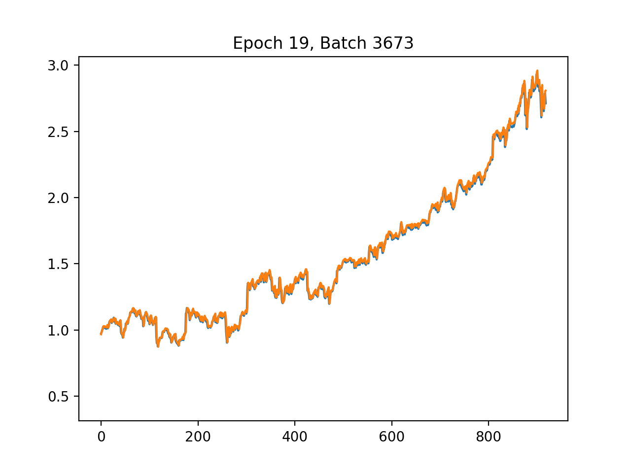
plt.ion()
fig = plt.figure()
ax1 = fig.add_subplot(111)
line1, = ax1.plot(y_test)
line2, = ax1.plot(y_test * 0.5)
plt.show()
batch_size = 1
mse_train = []
mse_test = []
epochs = 20
for e in range(epochs):
shuffle_indices = np.random.permutation(np.arange(len(y_train)))
X_train = X_train[shuffle_indices]
y_train = y_train[shuffle_indices]
for i in range(0, len(y_train) // batch_size):
start = i * batch_size
batch_x = X_train[start:start + batch_size]
batch_y = y_train[start:start + batch_size]
net.run(opt, feed_dict={X: batch_x, Y: batch_y})
mse_train.append(net.run(mse, feed_dict={X: X_train, Y: y_train}))
mse_test.append(net.run(mse, feed_dict={X: X_test, Y: y_test}))
print(’Epoch ‘ + str(e))
print(’MSE Train: ‘, mse_train[-1])
print(’MSE Test: ‘, mse_test[-1])
pred = net.run(out, feed_dict={X: X_test})
rel_error = abs(np.mean(((pred - y_test) / y_test)))
print(’Relative error: ‘ + str(”{:.2%}”.format(rel_error)))
line2.set_ydata(pred)
plt.title(’Epoch ‘ + str(e) + ‘, Batch ‘ + str(i))
plt.pause(0.001)
pred_final = net.run(out, feed_dict={X: X_test})
rel_error = abs(np.mean(((pred_final - y_test) / y_test)))
mse_final = net.run(mse, feed_dict={X: X_test, Y: y_test})
print(’Final MSE test: ‘ + str(mse_final))
print(’Final Relative error: ‘ + str(”{:.2%}”.format(rel_error)))
print(’Total training set count: ‘ + str(len(y_train)))
print(’Total test set count: ‘ + str(len(y_test)))
savemodel(net, export_dir)
elapsed = time.time() - start_time
print(’time elapsed: ‘ + str(round(elapsed, 2)) + “ seconds”)As the TensorFlow training routine invoked by train_batch, train orchestrates the full lifecycle of fitting a single stock’s neural network using the preprocessed train and test DataFrames supplied by train_batch. It first extracts the supervised target by pulling the label column into y_train and y_test and then removes that column so the remaining columns become the feature matrices X_train and X_test; it also captures the feature dimension p to size the input. The function builds a TensorFlow 1.x style computation graph and session: it creates placeholders named X and Y with shapes matching the feature matrix and scalar target, initializes three fully connected hidden layers with 64, 32 and 16 neurons respectively using a variance-scaling weight initializer and zero biases, applies ReLU activations, and wires a single-unit linear output node named out. It defines mean squared error as the loss named mse and uses the Adam optimizer to minimize that loss, then starts a Session and initializes variables. For live feedback during optimization it enables interactive Matplotlib plotting, drawing the true test targets and a second line that will be overwritten with model predictions each epoch. The training loop runs for a fixed number of epochs (shuffling the training set each epoch), iterates minibatches (batch size 1 here), runs the optimizer on each minibatch, and after each epoch computes and prints train and test MSE, produces predictions on X_test, computes a mean relative error, and updates the plot title and prediction line. After the epochs complete it computes final predictions and metrics, logs dataset sizes and final error numbers, and persists the trained model by calling savemodel with the current Session and the provided export_dir. The use of explicit tensor names and the TensorFlow Saver/Session pattern is what allows the complementary evaluate routine to later restore the graph, fetch tensors by name, and score the saved model. Finally, train reports the elapsed wall-clock time before returning.
# file path: scripts/neural_network.py
def savemodel(sess, export_dir):
    saver = tf.train.Saver()
    saver.save(sess, export_dir + ‘/MSFT’)
    print(’Saved model to ‘ + export_dir)
savemodel is the thin persistence step the training module uses to write a trained TensorFlow model to disk: it accepts the active TensorFlow session and an export directory, creates a TensorFlow Saver object to capture the session’s variables, and invokes the saver to write the session state into the export directory using a fixed base name of MSFT; after the checkpoint files are written it prints a confirmation that includes the export directory. In the pipeline this is called by train at the end of a single-symbol training run so the per-stock session state produced by train is persisted for later evaluation or inference; train_batch arranges a per-symbol export_dir (using format_path as explained earlier) and calls train, which in turn calls savemodel. The side effects are the creation of standard TensorFlow checkpoint artifacts on disk and a console message confirming the save.
# file path: scripts/utils.py
def remove_dir(path_from_root):
    shutil.rmtree(format_path(path_from_root), ignore_errors=True)
remove_dir takes a project-relative path and removes the filesystem tree at that location as a side effect. It first turns the incoming path fragment into an absolute path by calling format_path (which you already looked at), then delegates the actual deletion to the standard library recursive remover; the call is configured to ignore errors so the call is safe to run even when the target does not exist. In the pipeline this is the cleanup counterpart to make_dir_if_not_exists: where make_dir_if_not_exists ensures a directory exists for outputs, remove_dir clears out old outputs (for example the model export directory used by train_batch and evaluate_batch) so subsequent training or evaluation runs start from a clean state. There is no branching or return value — it’s a single, best-effort recursive delete operation that suppresses missing-file errors and leaves the rest of the batch flow to create or repopulate the directory as needed.
# file path: scripts/neural_network.py
if __name__ == ‘__main__’:
    train_batch(str(sys.argv[1]), str(sys.argv[2]), str(sys.argv[3]))
When the module is run as a standalone script the bottom-level entry point grabs three positional command-line values and hands them to train_batch so the file can be used to kick off the per-symbol training loop directly. In practice those three arguments map to the symbols list file, the directory containing the preprocessed train/test CSVs, and the export directory where each symbol’s model artifacts will be written; train_batch will then iterate the symbols, load each symbol’s train and test CSVs, remove any existing model directory for that symbol, and call train to fit a TensorFlow network and persist its outputs. This mirrors the earlier module-level entry guard pattern you saw that forwarded sys.argv into fetch, but differs from the run.py main function which uses option parsing and calls neural_network.train_batch with hard-coded paths; the entry point here provides a lightweight, positional-argument way to run the batch training flow from the command line.
# file path: scripts/plot.py
import sys
import pandas as pd
import matplotlib.pyplot as plt
from utils import format_path
The file pulls in a very small, focused set of runtime helpers that match its role as a visualization utility: sys provides access to interpreter-level functionality such as command-line arguments and process control so the plotting routine can be invoked from the shell or a wrapper script; pandas is used to read and manipulate the time-indexed actual and predicted adjusted-close series so the data can be aligned, sliced, and prepared for plotting; matplotlib.pyplot supplies the plotting primitives and figure management used to render and persist the actual-versus-predicted charts; and format_path from utils is the project-level helper that canonicalizes the model/output file locations so plot_closing_adj can find the saved predictions and metadata. This import set is intentionally lean compared with other modules that also pull in training/runtime dependencies — for example, some files add tensorflow, numpy, or additional filesystem helpers from utils and constants for training and directory management — but plot_closing_adj follows the common project pattern of always importing sys and pandas while avoiding heavy ML libraries because its sole responsibility is loading already-produced outputs and rendering them.
# file path: scripts/plot.py
def plot_closing_adj(path_to_csv):
    data = pd.read_csv(format_path(path_to_csv), index_col=’date’)
    print(’plotting data for ‘ + path_to_csv + ‘...’)
    print(’data dimensions ‘ + str(data.shape))
    plt.plot(data.index.values, data[’adjusted’].values)
    plt.show()
plot_closing_adj is the simple visualization helper used in the evaluation/visualization stage of the pipeline: it accepts a path_to_csv (expected relative to the repository root), uses format_path to turn that into an absolute filesystem path consistent with other IO helpers, and then loads the CSV into a pandas DataFrame with the date column as the index. After loading it prints a short console message identifying which CSV is being plotted and another showing the DataFrame dimensions, then renders the time series by plotting the DataFrame index against the DataFrame’s adjusted column and calling the plotting library’s show routine so the figure is displayed to the user. There are no branches or return values—its side effects are the console output and the blocking plot window—and it fits into the pipeline as the quick way to view the actual adjusted-close series for a symbol during or after training/evaluation (it relies on format_path the same way other batch utilities do to locate files).
This Substack is reader-supported. To receive new posts and support my work, consider becoming a free or paid subscriber.
# file path: scripts/plot.py
if __name__ == ‘main’:
    plot_closing_adj(str(sys.argv[1]))
The snippet performs a runtime check of the module-level name variable to decide whether the file was invoked as a script; when that check passes it invokes plot_closing_adj with the first command-line argument taken from sys.argv. That call hands a user-supplied path into plot_closing_adj, which in turn uses format_path, pandas and matplotlib to load the saved series (model/output CSV) and render the actual versus predicted adjusted-close trace for quick visual inspection. Functionally this provides a minimal command-line visualization entry point: you run the file with a single path and the plotting routine displays the series. This mirrors the pattern used by the other module-level guard that forwards argv values into fetch, but differs in that the other guard expects three positional arguments and launches the fetch pipeline, whereas this one expects a single path and launches the plotting/visualization step; if the name check does not pass (for example when the module is imported), nothing is executed.
# file path: scripts/preprocess.py
def fill_missing(data):
    data.fillna(method=’ffill’, inplace=True)
    data.fillna(method=’bfill’, inplace=True)
    data.fillna(value=0, inplace=True)
    return data
fill_missing is the simple imputation step that sits immediately after construct_label inside preprocess and prepares the labeled DataFrame for splitting and scaling. It accepts the pandas DataFrame coming out of construct_label and applies three deterministic passes to eliminate missing values: first it forward-fills to carry the most recent observed value forward across gaps (preserving temporal continuity for features), then it backward-fills to populate any leading gaps that forward-fill cannot touch, and finally it replaces any remaining missing entries with zero so there are no NaNs left for downstream consumers. The ordering matters because it prefers to reuse nearby observed values when available and only falls back to a constant when no nearby observation exists. fill_missing mutates the DataFrame in place and returns it unchanged structurally (index and columns preserved), which is important because split relies on the original time index and scale expects dense numeric inputs to fit and transform. There is no branching or error handling here—just a fixed, repeatable imputation pipeline designed to make the per-symbol data safe for the subsequent split and MinMaxScaler stages.
# file path: scripts/preprocess.py
def scale(train_data, test_data):
    scaler = MinMaxScaler()
    scaler.fit(train_data)
    train_data_np = scaler.transform(train_data)
    test_data_np = scaler.transform(test_data)
    train_data = pd.DataFrame(train_data_np, index=train_data.index, columns=train_data.columns)
    test_data = pd.DataFrame(test_data_np, index=test_data.index, columns=test_data.columns)
    return train_data, test_data
scale accepts the train_data and test_data DataFrames produced earlier in preprocess (after construct_label, fill_missing, and split) and normalizes feature columns for modeling. It instantiates a MinMaxScaler and fits it only on train_data so the per-feature minima and maxima are learned from the training set; it then applies that fitted scaler to transform both the training and the held-out test partitions so the test set is scaled using training-derived parameters (preventing target leakage). The raw transform produces NumPy arrays, which scale wraps back into pandas DataFrames while preserving the original row indices and column names so downstream consumers keep the date index and feature labels intact. It returns the scaled train and test DataFrames ready for the per-symbol training and evaluation stages; because MinMaxScaler is used, features end up normalized to the standard 0–1 range determined by the training data.
# file path: scripts/preprocess.py
def construct_label(data):
    data[’label’] = data[’adjusted’]
    data[’label’] = data[’label’].shift(-1)
    return data.drop(data.index[len(data)-1])
construct_label turns the raw adjusted-close series into the supervised learning target the pipeline expects: it creates a new column named label by copying the existing adjusted values and then shifts that column so each row’s label represents the next trading day’s adjusted close. Because shifting produces a missing value at the end of the series, construct_label removes the final row so every remaining record has a valid next-day target. This labeled DataFrame is what preprocess receives next (preprocess then calls fill_missing to propagate any missing feature values, split to partition by train_ratio, and scale to fit and apply a MinMaxScaler), and the one-row reduction caused by dropping the last index affects the subsequent split and scaling steps.
# file path: scripts/preprocess.py
def preprocess(data, train_ratio):
    data = construct_label(data)
    data = fill_missing(data)
    train_data, test_data = split(data, train_ratio)
    train_data, test_data = scale(train_data, test_data)
    return train_data, test_data
preprocess is the per-symbol orchestration that turns a raw, time-indexed DataFrame into the paired, scaled train and test sets the rest of the pipeline expects. It receives the DataFrame that preprocess_batch loaded (date as index and columns including the adjusted-close series) and first calls construct_label to create the next-day supervised target: the adjusted-close value is copied into a new label column and shifted so each row’s label corresponds to the following trading day, and the trailing row that loses its label is removed. After the label exists, preprocess calls fill_missing to make the series contiguous for modeling by forward-filling, then back-filling, and finally replacing any remaining gaps with zero so no NaNs remain. Next it delegates to split with the provided train_ratio to slice the time-ordered rows into an earlier training portion and a later test portion (a simple row-index split so the temporal order is preserved). Finally preprocess calls scale which fits a MinMaxScaler on the training DataFrame only, transforms both sets with that fitted scaler to avoid leakage, and wraps the scaled arrays back into pandas DataFrames that keep the original row indices and column names. The function then returns the scaled train and test DataFrames, ready for train_batch to persist and for the neural-network training and later evaluation steps to consume.
# file path: scripts/preprocess.py
def preprocess_batch(input_path, output_path, train_ratio):
    start = time.time()
    files = get_filename_list(input_path, ‘csv’)
    for file in files:
        symbol = file.split(’.’)[0]
        print(”preprocessing “ + symbol)
        data = pd.read_csv(format_path(input_path + ‘/’ + file), index_col=’date’)
        train_data, test_data = preprocess(data, train_ratio)
        formatted_output = format_path(output_path)
        make_dir_if_not_exists(formatted_output + ‘/train’)
        make_dir_if_not_exists(formatted_output + ‘/test’)
        train_data.to_csv(formatted_output + ‘/train’ + ‘/’ + symbol + ‘.csv’)
        test_data.to_csv(formatted_output + ‘/test’ + ‘/’ + symbol + ‘.csv’)
        print(’saved csv files to ‘ + formatted_output + ‘{train, test}/’ + symbol + ‘.csv’)
    print(”preprocessing complete”)
    elapsed = time.time() - start
    print(’time elapsed: ‘ + str(round(elapsed, 2)) + “ seconds”)
preprocess_batch is the orchestration routine that turns a directory of raw per-symbol CSVs into the scaled, labeled train and test CSVs the rest of the pipeline expects. It starts a timer, enumerates CSV filenames using get_filename_list, and then iterates over those files; for each file it derives the symbol name, prints a progress message, and loads the CSV into a pandas DataFrame with the date index using format_path to canonicalize the filesystem access. The loaded DataFrame is handed to preprocess, which is responsible for constructing the next-day label, filling missing values, splitting into train and test, and scaling features, and preprocess_batch receives back a train_data and a test_data DataFrame. preprocess_batch then ensures the standardized output layout exists by formatting the output root and invoking make_dir_if_not_exists for the train and test subdirectories, writes the two DataFrames out as symbol-named CSVs into those subdirectories, and prints a confirmation for each symbol. After all files are processed it prints completion and the elapsed time. The produced train and test CSVs are the inputs consumed by downstream batch stages such as train_batch and evaluate_batch, so preprocess_batch enforces the consistent preprocessing, splitting, scaling, and file organization that the model training and evaluation steps rely on.
# file path: scripts/utils.py
def get_filename_list(path_from_root, suffix) -> list:
    filenames = os.listdir(format_path(path_from_root))
    return [filename for filename in filenames if filename.endswith(suffix)]
get_filename_list is a small filesystem helper that the batch stages use to discover which files in a project-relative directory should be processed. It first uses format_path to turn the provided project-relative path into an absolute directory, lists the directory contents, and then returns only the entries whose names end with the provided suffix. preprocess_batch calls get_filename_list with a csv suffix to obtain the set of symbol CSV filenames to iterate over; each returned filename is then turned into a symbol name, loaded via format_path, and sent through preprocess and the rest of the pipeline. Its role is to centralize simple file discovery and suffix-based filtering so the various batch operations don’t duplicate directory listing logic, following the same helper-style pattern used by format_path and make_dir_if_not_exists.
# file path: scripts/run.py
import sys
import getopt
import time
import fetch_combined_data
import preprocess
import neural_network
import evaluate_neural_network
The imports at the top wire the script into the command-line orchestration role of the pipeline: sys provides access to interpreter-level features such as reading argv and terminating the process when argument parsing fails, while getopt is used to parse the short and long command-line flags that select which pipeline stages to run. time is pulled in so the script can measure and report elapsed wall-clock time for the run. The remaining four imports are the project-level stage modules that implement the pipeline steps: fetch_combined_data contains the data acquisition routines that gather symbol and indicator feeds into the raw output area; preprocess exposes the preprocessing pipeline that fills gaps, constructs labels, scales features, and splits sequences (the stage invoked by preprocess_batch); neural_network implements the per-stock model training logic (the stage invoked by train_batch); and evaluate_neural_network provides the evaluation/visualization step that consumes trained models and test splits to produce metrics and plots (the stage invoked by evaluate_batch). Together these imports reflect the procedural orchestrator pattern used by run.py: command-line parsing and timing control locally, and delegation of each major pipeline phase to a dedicated module that encapsulates the implementation details. This is the same high-level pattern you saw in the main function: getopt-driven flags trigger calls into fetch_combined_data, preprocess, neural_network, and evaluate_neural_network to perform fetch → preprocess → train → evaluate, and when the module is invoked directly the bottom-level entry point delegates arguments into the training path as noted earlier.
# file path: scripts/run.py
def main(argv):
    start = time.time()
    try:
        opts, _ = getopt.getopt(argv, ‘fpn’, [’fetch’, ‘preprocess’, ‘neuralnetwork’, ‘evalnn’])
    except getopt.GetoptError:
        print(’run.py’)
        sys.exit(2)
    print(’-----command line options-----’)
    print(opts)
    single_opt = [opt[0] for opt in opts]
    if ‘-f’ in single_opt or ‘--fetch’ in single_opt:
        print(’-----fetching new data-----’)
        fetch_combined_data.fetch(
            ‘input/symbols’,
            ‘input/indicators’,
            ‘output/raw’
        )
    if ‘-p’ in single_opt or ‘--preprocess’ in single_opt:
        print(’-----preprocessing data-----’)
        preprocess.preprocess_batch(
            ‘output/raw’,
            ‘output/preprocessed’,
            0.8
        )
    if ‘-n’ in single_opt or ‘--neuralnetwork’ in single_opt:
        print(’-----training Neural Network models-----’)
        neural_network.train_batch(
            ‘input/symbols’,
            ‘output/preprocessed’,
            ‘output/models’
        )
    if ‘--evalnn’ in single_opt:
        print(’-----Evaluating Neural Network models-----’)
        evaluate_neural_network.evaluate_batch(
            ‘input/symbols’,
            ‘output/preprocessed/test’
        )
    elapsed = time.time() - start
    print(’time elapsed: ‘ + str(round(elapsed, 2)) + “ seconds”)
    print(’-----program finished-----’)
main orchestrates the staged pipeline by parsing command-line flags, deciding which stages to run, invoking the concrete batch helpers, and reporting elapsed time. It starts a timer, then uses getopt to accept short flags for fetch, preprocess, and neuralnetwork and a long flag for evalnn; if option parsing fails it prints a small help-like line and exits with status code 2. After printing the parsed options it reduces the getopt output to a simple list of option names and then conditionally executes the stages in a fixed order: if the fetch flag is present it calls fetch_combined_data.fetch to pull combined symbol and indicator feeds and write them into the raw output directory; if the preprocess flag is present it calls preprocess.preprocess_batch to turn the raw CSVs into train/test splits and scaled feature files (the call supplies the raw input directory, the preprocessed output directory, and a train ratio of 0.8); if the neuralnetwork flag is present it calls neural_network.train_batch to iterate over the symbol list and train a TensorFlow model per ticker, exporting each model into the models directory; and if the evalnn long flag is present it calls evaluate_neural_network.evaluate_batch to run per-symbol evaluation against the test set under output/preprocessed/test. After any enabled stages complete it prints the elapsed wall-clock time and a finished message. The control flow therefore supports running any subset of the pipeline stages
# file path: scripts/run.py
if __name__ == ‘__main__’:
    main(sys.argv[1:])
The module-execution guard at gap_L48_49 ensures that when scripts/run.py is executed directly it invokes main and passes the command-line arguments excluding the interpreter-invoked program name; main then becomes responsible for parsing those arguments and driving the staged workflow (preprocess_batch, train_batch, evaluate_batch) according to what the caller requested. This preserves the file’s dual role as an importable set of orchestration helpers and as a standalone pipeline driver, preventing automatic execution when other modules import symbols from scripts/run.py. Compared with the other entry points you saw earlier—one that invoked plot_closing_adj with a single argv value and the bottom-level entry that forwarded three positional values directly to train_batch—this guard delegates the entire argv tail to main, giving main the flexibility to validate, parse, and route a variable argument shape into the batch preprocessing/training/evaluation sequence.
# file path: setup/setup.sh
echo
echo --------------------🇨🇳 Database Setup🇨🇳 --------------------
echo 😊 Enter your custom configurations when prompted, otherwise hit ‘enter’ to use default.
read -p “Database hostname (localhost): “ database
read -p “Database user (root): “ user
read -s -p “Database password: “ pass
echo
echo
LOGWRITE=”DEV_DB_HOST=${database:=’localhost’}\nDEV_DB_USER=${user:=’root’}\nDEV_DB_PASS=lol i ain’t showing you shit\n”
echo $LOGWRITE
echo “🤔 Running database setup”;
echo
export MYSQL_PWD=$pass
echo 🚴 Setting up database...
mysql -u $user < setup.sql
echo 📚 Completed
unset MYSQL_PWD
echo -------------------🇨🇳 Setup completed🇨🇳  --------------------
setup.sh is an interactive shell bootstrap that prepares the MySQL-backed runtime the pipeline expects before any preprocessing, training, or evaluation runs. It walks the operator through entering a database hostname, username, and a silent password prompt, applying sensible defaults for host and user when the operator hits enter; it then assembles a small status string that reports the selected host and user while explicitly masking the password when printed to the console. The script exports the entered password into the MYSQL_PWD environment variable so the mysql client can be invoked non-interactively with the supplied username and the setup SQL file, effectively initializing the database schema and any baseline data the project needs. After the mysql client runs, the script clears the password environment variable and emits human-friendly progress and completion messages (with emoji), leaving the filesystem and environment ready for the pipeline’s fetch→preprocess→train→evaluate sequence. Because setup.sh is a standalone interactive initializer rather than a library helper like remove_dir or the plotting utilities, it is intended to be run once by an operator to create and seed the database dependencies that later pipeline stages rely on.
Use the button below to download:
