

Covid-19 Infected Person? Find Using Images & Densenet-121 Neural Network
The Covid-19 pandemic has caused widespread health and economic devastation around the world.

One of the biggest challenges in controlling the spread of the virus has been identifying infected individuals quickly and accurately. In this article, we explore how deep learning techniques can be used to analyze medical images and scans to detect Covid-19 in patients. Specifically, we’ll be using the DenseNet-121 neural network to analyze chest x-rays and CT scans.
Watch My Video here:
Imports
# This Python 3 environment comes with many helpful analytics libraries installed
# It is defined by the kaggle/python Docker image: https://github.com/kaggle/docker-python
# For example, here's several helpful packages to load

import numpy as np # linear algebra
import pandas as pd # data processing, CSV file I/O (e.g. pd.read_csv)

# Input data files are available in the read-only "../input/" directory
# For example, running this (by clicking run or pressing Shift+Enter) will list all files under the input directory

import os
#for dirname, _, filenames in os.walk('/kaggle/input'):
    #for filename in filenames:
        #print(os.path.join(dirname, filename))

# You can write up to 5GB to the current directory (/kaggle/working/) that gets preserved as output when you create a version using "Save & Run All"
# You can also write temporary files to /kaggle/temp/, but they won't be saved outside of the current session
#importing necessary python libraries.
import numpy as np
import pandas as pd
import matplotlib.pyplot as plt
%matplotlib inline # this line is used to display plots/graphs within the jupyter notebook itself.
import seaborn as sns
import cv2
import os
from tqdm import tqdm # Just a progress bar library that shows a progress meter during processing.
from sklearn.metrics import confusion_matrix # To compute confusion matrix to evaluate the accuracy of classification.
from sklearn.model_selection import train_test_split # To split data into training and testing sets.
from keras.utils.np_utils import to_categorical # Used for one-hot encoding the labels.
from keras.models import Model,Sequential, Input, load_model # importing deep learning model from keras
from keras.layers import Dense, Dropout, Flatten, Conv2D, MaxPool2D, BatchNormalization, AveragePooling2D, GlobalAveragePooling2D
from keras.optimizers import Adam # optimization algorithm to minimize loss function
from keras.preprocessing.image import ImageDataGenerator # used for generating augmented images
from keras.callbacks import ModelCheckpoint, ReduceLROnPlateau # used to save the best weights of model and reduces learning rate when improvment stops
from keras.applications import DenseNet121 # Pretrained Deep Learning ModelImporting Data
disease_types=['COVID', 'non-COVID']
data_dir = '/kaggle/input/sarscov2-ctscan-dataset/SARS-Cov-2/'
train_dir = os.path.join(data_dir)
train_data = []
for defects_id, sp in enumerate(disease_types):
for file in os.listdir(os.path.join(train_dir, sp)):
train_data.append(['{}/{}'.format(sp, file), defects_id, sp])
train = pd.DataFrame(train_data, columns=['File', 'DiseaseID','Disease Type'])
train.head()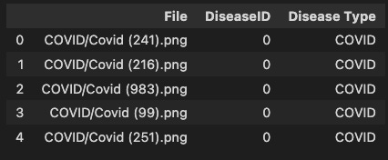
This code snippet is used to create a list of image file paths and corresponding disease labels from a dataset of COVID-19 diagnosis images. The dataset is organized into folders, where each folder corresponds to a specific disease type (e.g., normal, COVID-19). Here’s a breakdown of the code:
train_data = []: An empty list called train_data is created to store the information about each image file and its corresponding disease type.
for defects_id, sp in enumerate(disease_types):: This for loop iterates through the disease_types list, which contains the names of the disease folders in the dataset. The enumerate() function is used to get both the index (stored in defects_id) and the disease folder name (stored in sp) for each iteration.
for file in os.listdir(os.path.join(train_dir, sp)): This nested for loop iterates through each file in the current disease folder. os.listdir() lists all the files in the folder specified by os.path.join(train_dir, sp), where train_dir is the root directory containing all disease folders, and sp is the current disease folder name.
train_data.append([‘{}/{}’.format(sp, file), defects_id, sp]): For each file (image) in the current disease folder, a list containing the relative file path (‘{}/{}’.format(sp, file)), the disease index (defects_id), and the disease name (sp) is appended to the train_data list.
train = pd.DataFrame(train_data, columns=[‘File’, ‘DiseaseID’, ‘Disease Type’]): Once all the files and their corresponding disease information have been added to the train_data list, a pandas DataFrame named train is created. The DataFrame has three columns: ‘File’ for the relative file path, ‘DiseaseID’ for the disease index, and ‘Disease Type’ for the disease name.
train.head(): This line displays the first 5 rows of the train DataFrame to provide a glimpse of the data. This is helpful to ensure that the DataFrame was created correctly and that the data is in the expected format.
In summary, this code snippet creates a pandas DataFrame containing the file paths and corresponding disease labels for a dataset of COVID-19 diagnosis images organized in folders by disease type.
Randomizing
SEED = 42
train = train.sample(frac=1, random_state=SEED)
train.index = np.arange(len(train)) # Reset indices
train.head()
This code snippet is responsible for shuffling the train DataFrame created in the previous snippet to ensure that the order of the data is randomized. Randomizing the order of the data is important in machine learning to avoid any potential bias due to the initial ordering of the dataset. Here’s a breakdown of the code:
SEED = 42: This line sets a constant value called SEED to 42. The purpose of this seed value is to ensure that the randomization process is reproducible. By using the same seed value, you can obtain the same random order of the dataset every time you run the code.
train = train.sample(frac=1, random_state=SEED): The sample() function is called on the train DataFrame to shuffle its rows. The frac parameter is set to 1, which means that all the rows in the DataFrame should be included in the shuffled output. The random_state parameter is set to the SEED value (42) to ensure reproducibility.
train.index = np.arange(len(train)): This line resets the index of the train DataFrame after shuffling. The np.arange() function creates a new numpy array with consecutive integers from 0 to len(train) — 1, which is the total number of rows in the DataFrame. This new array is assigned to the index property of the DataFrame, effectively resetting the indices to a new sequence of consecutive integers.
train.head(): This line displays the first 5 rows of the shuffled train DataFrame, allowing you to verify that the DataFrame has indeed been randomized.
In summary, this code snippet shuffles the train DataFrame containing the file paths and corresponding disease labels for a dataset of COVID-19 diagnosis images, ensuring that the order of the data is randomized to avoid bias. It also resets the DataFrame indices and displays the first 5 rows of the shuffled data.
Plotting a Histogram
plt.figure(figsize=(12, 12))
plt.hist(train['DiseaseID'])
plt.title('Frequency Histogram of Species')
plt.show()
This code snippet is responsible for creating and displaying a histogram of the disease labels (DiseaseID) present in the train DataFrame. A histogram is a graphical representation of the distribution of a dataset, and in this case, it helps to visualize the number of images per disease type in the dataset. Here’s a breakdown of the code:
plt.hist(train[‘DiseaseID’]): The plt.hist() function from the matplotlib.pyplot library (imported as plt) is used to create a histogram of the ‘DiseaseID’ column from the train DataFrame. The ‘DiseaseID’ column contains integer labels representing different disease types.
plt.title(‘Frequency Histogram of Species’): This line sets the title of the histogram plot to ‘Frequency Histogram of Species’ using the plt.title() function.
plt.figure(figsize=(12, 12)): The plt.figure() function is called with the figsize parameter set to (12, 12), which creates a new figure with the specified width and height in inches. However, this line should be placed before the plt.hist() function call to properly set the figure size for the histogram plot.
plt.show(): This line displays the histogram plot using the plt.show() function.
In summary, this code snippet creates and displays a histogram of the disease labels (DiseaseID) present in the train DataFrame to visualize the distribution of the dataset. The plot shows the number of images per disease type, which helps to understand the dataset’s balance.
Displaying Images Of COVID
def plot_defects(defect_types, rows, cols):
    fig, ax = plt.subplots(rows, cols, figsize=(12, 12))
    defect_files = train['File'][train['Disease Type'] == defect_types].values
    n = 0
    for i in range(rows):
        for j in range(cols):
            image_path = os.path.join(data_dir, defect_files[n])
            ax[i, j].set_xticks([])
            ax[i, j].set_yticks([])
            ax[i, j].imshow(cv2.imread(image_path))
            n += 1
# Displays first n images of class from training set
plot_defects('COVID', 5, 5)
This code snippet defines a function called plot_defects that displays a grid of images for a specific disease type from the train DataFrame. The purpose of this function is to help you visually inspect the images in the dataset. Here’s a breakdown of the code:
def plot_defects(defect_types, rows, cols):: The plot_defects function is defined with three parameters: defect_types, which represents the disease type (e.g., ‘COVID’); rows, the number of rows in the image grid; and cols, the number of columns in the image grid.
fig, ax = plt.subplots(rows, cols, figsize=(12, 12)): The plt.subplots()function is called to create a grid of subplots with the specified rows and cols values. The figsize parameter is set to (12, 12) to specify the width and height of the figure in inches. The function returns a Figure object (fig) and an array of Axes objects (ax).
defect_files = train[‘File’][train[‘Disease Type’] == defect_types].values: This line filters the ‘File’ column of the train DataFrame to select only the rows where the ‘Disease Type’ column equals the specified defect_types. The .values attribute is used to get the underlying numpy array of filtered file paths.
n = 0: A counter variable n is initialized to 0. This variable is used to iterate through the selected image file paths.
The nested for loops iterate through the rows and cols of the grid of subplots:
for i in range(rows): iterates through the rows of the grid.
for j in range(cols): iterates through the columns of the grid.
Inside the nested for loops:
image_path = os.path.join(data_dir, defect_files[n]): The os.path.join()function is called to concatenate the root directory data_dir and the current image file path defect_files[n] to get the full path of the image.
ax[i, j].set_xticks([]): This line removes the x-axis ticks from the current subplot.
ax[i, j].set_yticks([]): This line removes the y-axis ticks from the current subplot.
ax[i, j].imshow(cv2.imread(image_path)): The cv2.imread() function reads the image at the specified image_path. The imshow() function is then called on the current Axes object (ax[i, j]) to display the image in the subplot.
n += 1: The counter variable n is incremented by 1 to move to the next image file path.
plot_defects(‘COVID’, 5, 5): The plot_defects function is called with the parameters ‘COVID’ (the disease type), 5 (the number of rows in the image grid), and 5 (the number of columns in the image grid). This call displays a 5x5 grid of images from the ‘COVID’ disease type in the dataset.
In summary, this code snippet defines a function called plot_defects that displays a grid of images for a specific disease type from the train DataFrame. The function is called to display a 5x5 grid of images from the ‘COVID’ disease type.
Displaying Images of Non-COVID
def plot_defects(defect_types, rows, cols):
    fig, ax = plt.subplots(rows, cols, figsize=(12, 12))
    defect_files = train['File'][train['Disease Type'] == defect_types].values
    n = 0
    for i in range(rows):
        for j in range(cols):
            image_path = os.path.join(data_dir, defect_files[n])
            ax[i, j].set_xticks([])
            ax[i, j].set_yticks([])
            ax[i, j].imshow(cv2.imread(image_path))
            n += 1
# Displays first n images of class from training set
plot_defects('non-COVID', 5, 5)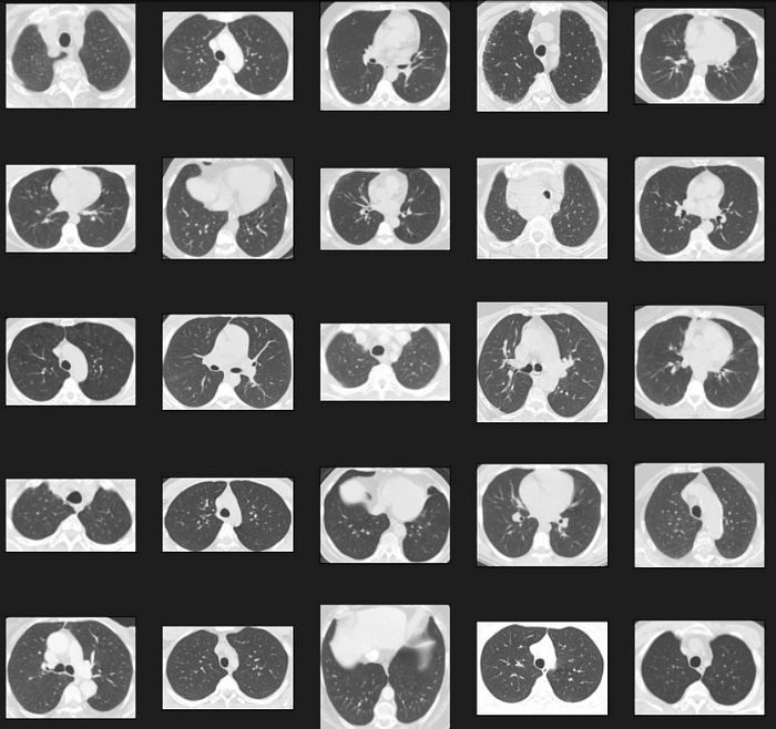
This code snippet is almost identical to the previous one, with the only difference being the disease type passed to the plot_defects() function. In this case, the function is called to display a 5x5 grid of images from the ‘non-COVID’ disease type. Here’s the breakdown of the code that is different from the previous snippet:
plot_defects(‘non-COVID’, 5, 5): The plot_defects function is called with the parameters ‘non-COVID’ (the disease type), 5 (the number of rows in the image grid), and 5 (the number of columns in the image grid). This call displays a 5x5 grid of images from the ‘non-COVID’ disease type in the dataset.
In summary, this code snippet defines a function called plot_defects that displays a grid of images for a specific disease type from the train DataFrame. The function is called to display a 5x5 grid of images from the ‘non-COVID’ disease type.
Image Read And Resize Function
IMAGE_SIZE = 64
def read_image(filepath):
    return cv2.imread(os.path.join(data_dir, filepath)) # Loading a color image is the default flag
# Resize image to target size
def resize_image(image, image_size):
    return cv2.resize(image.copy(), image_size, interpolation=cv2.INTER_AREA)
This code snippet defines two utility functions, read_image() and resize_image(), that are used for reading and resizing images from the dataset, respectively. Here’s a breakdown of the code:
IMAGE_SIZE = 64: This line sets a constant value called IMAGE_SIZE to 64. This value will be used later to resize images to a fixed size (64x64 pixels) for model training.
def read_image(filepath):: The read_image() function is defined with a single parameter, filepath, which is the relative path of an image file.
return cv2.imread(os.path.join(data_dir, filepath)): The cv2.imread()function is called to read the image file specified by the filepath parameter. The os.path.join() function is used to concatenate the root directory data_dir and the relative file path filepath to form the full path of the image. The cv2.imread() function returns the loaded image as a numpy array.
def resize_image(image, image_size):: The resize_image() function is defined with two parameters: image, which is the input image as a numpy array; and image_size, which is the target size for the resized image (both width and height, as they are assumed to be equal in this case).
return cv2.resize(image.copy(), image_size, interpolation=cv2.INTER_AREA): The cv2.resize() function is called to resize the input image to the specified image_size. The .copy() method is used to create a copy of the input image before resizing to avoid modifying the original image. The interpolation parameter is set to cv2.INTER_AREA, which is a recommended interpolation method for downsampling images.
In summary, this code snippet defines two utility functions for reading and resizing images from the dataset. The read_image() function reads an image file specified by a relative file path, while the resize_image() function resizes a given image to a specified target size using the cv2.INTER_AREAinterpolation method.
Training Images
X_train = np.zeros((train.shape[0], IMAGE_SIZE, IMAGE_SIZE, 3))
for i, file in tqdm(enumerate(train['File'].values)):
    image = read_image(file)
    if image is not None:
        X_train[i] = resize_image(image, (IMAGE_SIZE, IMAGE_SIZE))
# Normalize the data
X_Train = X_train / 255.
print('Train Shape: {}'.format(X_Train.shape))
This code snippet creates an array X_train that stores the resized and normalized images from the train DataFrame for further processing and model training. Here’s a breakdown of the code:
X_train = np.zeros((train.shape[0], IMAGE_SIZE, IMAGE_SIZE, 3)): A numpy array X_train of zeros is created with the shape (number of training samples, IMAGE_SIZE, IMAGE_SIZE, 3). The first dimension corresponds to the number of images in the training set, and the other dimensions represent the height, width, and number of color channels (3 for RGB) of the resized images.
for i, file in tqdm(enumerate(train[‘File’].values)):: A loop is created to iterate through the file paths in the ‘File’ column of the train DataFrame. The tqdm function wraps the enumerate() function to display a progress bar while looping through the file paths.
Inside the loop:
image = read_image(file): The read_image() function is called with the current file path to read the image.
if image is not None:: An if statement checks if the image is not None (i.e., the image was successfully read).
X_train[i] = resize_image(image, (IMAGE_SIZE, IMAGE_SIZE)): The resize_image() function is called with the loaded image and the target size (IMAGE_SIZE, IMAGE_SIZE). The resized image is then assigned to the corresponding position in the X_train array.
X_Train = X_train / 255.: The pixel values in the X_train array are normalized by dividing them by 255. This scales the pixel values to the range [0, 1], which can help improve the performance of the neural network during training. The normalized data is stored in a new array named X_Train.
print(‘Train Shape: {}’.format(X_Train.shape)): The shape of the X_Trainarray is printed to provide information about the dimensions of the processed dataset.
In summary, this code snippet creates an array X_train that stores the resized and normalized images from the train DataFrame. The images are read, resized, and normalized using the previously defined utility functions read_image() and resize_image(). The processed images are stored in a new array X_Train, which is ready for model training.
Converting Labels To Categorical
Y_train = train['DiseaseID'].values
Y_train = to_categorical(Y_train, num_classes=2)
This code snippet creates a one-hot encoded array Y_train for the disease labels (DiseaseID) in the train DataFrame. One-hot encoding is used to convert categorical integer labels into a binary vector that can be used as the target for model training. Here’s a breakdown of the code:
Y_train = train[‘DiseaseID’].values: This line extracts the ‘DiseaseID’ column from the train DataFrame as a numpy array and assigns it to the variable Y_train. The ‘DiseaseID’ column contains integer labels representing the different disease types (e.g., 0 for ‘COVID’, 1 for ‘non-COVID’).
Y_train = to_categorical(Y_train, num_classes=2): The to_categorical()function from the Keras library is called to convert the integer labels in Y_train into one-hot encoded vectors. The num_classes parameter is set to 2, as there are two disease types (‘COVID’ and ‘non-COVID’). The resulting one-hot encoded array is assigned back to the Y_train variable.
For example, if the original Y_train array contains the labels [0, 1, 0, 1],the one-hot encoded Y_train array would look like this:
[[1, 0],
[0, 1],
[1, 0],
[0, 1]]
In summary, this code snippet creates a one-hot encoded array Y_train for the disease labels (DiseaseID) in the train DataFrame. This one-hot encoded array can be used as the target for model training.
Train Test Splitting
BATCH_SIZE = 64

# Split the train and validation sets
X_train, X_val, Y_train, Y_val = train_test_split(X_Train, Y_train, test_size=0.2, random_state=SEED)
This code snippet splits the preprocessed dataset (X_Train and Y_train) into training and validation sets using the train_test_split function from the sklearn library. Validation sets are used to evaluate the model’s performance during training and help prevent overfitting. Here’s a breakdown of the code:
BATCH_SIZE = 64: A constant value BATCH_SIZE is set to 64. This value represents the number of samples that will be propagated through the model at each training iteration (also known as the batch size).
X_train, X_val, Y_train, Y_val = train_test_split(X_Train, Y_train, test_size=0.2, random_state=SEED): The train_test_split function is called with the following parameters:
X_Train: The array containing the resized and normalized images.
Y_train: The one-hot encoded array of disease labels.
test_size=0.2: This parameter specifies that 20% of the data will be used as the validation set.
random_state=SEED: The random seed is set to ensure reproducibility of the split.
The train_test_split function returns four arrays: X_train and Y_train for the training set, and X_val and Y_val for the validation set.
In summary, this code snippet splits the preprocessed dataset into training and validation sets using the train_test_split function. It also sets a constant value BATCH_SIZE to 64, which will be used later during model training.
64*64 Training Images
fig, ax = plt.subplots(1, 3, figsize=(15, 15))
for i in range(3):
    ax[i].set_axis_off()
    ax[i].imshow(X_train[i])
    ax[i].set_title(disease_types[np.argmax(Y_train[i])])
This code snippet displays the first three images from the X_train array along with their corresponding disease type labels. Here’s a breakdown of the code:
fig, ax = plt.subplots(1, 3, figsize=(15, 15)): A 1x3 grid of subplots is created using the plt.subplots() function, with a figure size of 15x15 inches. The function returns the figure object fig and an array of Axes objects ax.
for i in range(3):: A loop is created to iterate over the indices of the first three images in the X_train array.
Inside the loop:
ax[i].set_axis_off(): The axis is turned off for the current subplot using the set_axis_off() method. This hides the axis labels and ticks, providing a cleaner view of the image.
ax[i].imshow(X_train[i]): The imshow() method is called on the current Axes object to display the i-th image from the X_train array.
ax[i].set_title(disease_types[np.argmax(Y_train[i])]): The set_title()method is called on the current Axes object to set the title of the subplot. The title is the disease type corresponding to the i-th label in the Y_train array. The np.argmax() function is used to find the index of the maximum value in the one-hot encoded label, which corresponds to the original integer label. The disease_types list is then used to map the integer label back to the disease type string.
In summary, this code snippet displays the first three images from the X_train array along with their corresponding disease type labels in a 1x3 grid of subplots. The loop iterates over the first three images and displays them on the subplots with the disease type as the title.
EPOCHS = 50
SIZE=64
N_ch=3
This code snippet defines three constant values that will be used during model training:
EPOCHS = 50: The EPOCHS constant is set to 50, representing the number of times the entire training dataset will be passed through the model during training. Each epoch consists of multiple iterations (batches) covering the entire dataset.
SIZE = 64: The SIZE constant is set to 64, which is the same as the previously defined IMAGE_SIZE. This value represents the width and height of the resized images in the dataset.
N_ch = 3: The N_ch constant is set to 3, representing the number of color channels in the images (3 for RGB).
These constant values will be used as parameters in the DenseNet model or during the training process.