

Cracking the Complexity Code: Big O & Interview-Grade Analysis
Go beyond theory and learn how to estimate complexity from constraints, master amortized analysis, and spot hidden performance traps in Python and ML.

Download the entire book using the URL at the end of this article!
Big O, Big Theta, and Big Omega are shorthand for specific relations between two functions as their argument grows without bound. Use these definitions as tools for precise interview answers, not as rhetorical approximations.
f(n) ∈ O(g(n)) if there exist constants c > 0 and n0 such that for all n ≥ n0, f(n) ≤ c · g(n). This is an upper bound: f grows no faster than g up to constant factors for large n.
f(n) ∈ Ω(g(n)) if there exist constants c > 0 and n0 such that for all n ≥ n0, f(n) ≥ c · g(n). This is a lower bound: f grows at least as fast as g asymptotically.
f(n) ∈ Θ(g(n)) if f(n) ∈ O(g(n)) and f(n) ∈ Ω(g(n)). Θ denotes a tight bound; g captures the asymptotic growth rate of f up to constants.
Explicit constants and a domain assumption are part of a correct proof. Always state "for sufficiently large n" or give a numeric n0. In interviews, a compact proof sketch that identifies c and n0 is preferred to a hand-wavy claim.
Worked numeric example (compact proof style)
Take f(n) = 3n + 2. Show f ∈ O(n), f ∈ Ω(n), hence f ∈ Θ(n).
Upper bound (Big O): choose c = 5 and n0 = 1. For all n ≥ 1, 3n + 2 ≤ 3n + 2n = 5n = c·n. Therefore f(n) ≤ c·n for all n ≥ n0, so f ∈ O(n).
Lower bound (Big Omega): choose c = 3 and n0 = 1. For all n ≥ 1, 3n + 2 ≥ 3n = c·n. Therefore f(n) ≥ c·n for n ≥ n0, so f ∈ Ω(n).
Tight bound (Big Theta): since both relations hold, f ∈ Θ(n).
This is the concise proof style to deliver aloud: state your constants and domain, write the inequality, conclude. If asked for rigor, note that constants are not unique; any valid pair suffices.
Illustrative code (minimal, demonstrative)
The following snippet is only to make the inequality check explicit for small n—do not rely on finite checks for mathematical proof during interviews. It demonstrates picking constants and verifying the bound over a sample range to build confidence.
# Illustrative check: verifying chosen constants for f(n)=3n+2
def f(n): return 3*n + 2

c_upper, n0 = 5, 1
for n in range(n0, 100):
    assert f(n) <= c_upper * n

c_lower = 3
for n in range(n0, 100):
    assert f(n) >= c_lower * n
Why state constants and n0? Interviewers listen for explicit assumptions. Saying "choose c=5, n0=1" is short, precise, and demonstrates formal understanding.
Baseline-first coding scaffold
A repeatable mental scaffold orders problem solving and anchors complexity reasoning under interview pressure. Use these five steps in every coding problem:
Clarify: Restate the input types, bounds, and expected output. Ask about edge cases (empty input, negative values, duplicates) and resource constraints (memory, time limits).
Baseline: Give a simple correct solution with its complexity. This establishes correctness and an initial complexity reference.
Implement/Test: Code or pseudocode the baseline, run through a couple of small examples and edge cases verbally or on paper.
Complexity: State time and space for baseline. Give a short proof sketch (one or two inequalities or an amortized argument if relevant).
Optimize: Propose improvements, give their complexities, and trade-offs. Stop when improvements hit diminishing returns or constraints.
This scaffold enforces a complexity-first culture: clarify, then baseline, then justify costs before optimizing.
Five-bullet interview script for verbalizing complexity
When asked for complexity, fill these five bullets concisely; they form a 30–60 second verbal answer:
Assumptions: input sizes and relevant bounds (n is number of items, m number of edges; keys fit in memory; adversarial inputs possible?).
High-level complexity: state the tightest asymptotic bound you can (Θ(...) if you can justify both sides; otherwise use O(...) and mention average vs worst-case).
Proof sketch: give the inequality or amortized reasoning with constants or an iteration count (e.g., "each element is processed once; inner pointer only advances forward giving O(n) total").
Space: state auxiliary memory and whether solution is in-place; include recursion stack if recursive.
Edge-cases & mitigations: note adversarial cases (hash collisions, degenerate graphs), and fallback strategies (use balanced trees, change hashing, limit recursion depth).
Example fill-in for f(n) = 3n + 2:
Assumptions: n is integer ≥ 1.
High-level complexity: Θ(n).
Proof sketch: 3n+2 ≤ 5n for n≥1 so O(n); 3n+2 ≥ 3n so Ω(n); thus Θ(n).
Space: O(1) auxiliary.
Edge-cases: none nontrivial; constants irrelevant for asymptotics; mention runtime differences between languages.
Practice prompt (realistic interview rehearsal)
Time yourself: in 60 seconds, say the five bullets for a simple function or algorithm (for example, "binary search on sorted array" or "hash-based Two Sum"). Record the constants or amortized argument in the proof sketch bullet. Self-assess: did you state assumptions and space? Could an interviewer ask about average vs worst-case for your chosen data structures?
Practical notes and failure modes
Always separate asymptotic claims from implementation constants. Claiming O(n) in Python is correct asymptotically, but large constant factors—interpreted as unacceptable in a timed system—are legitimate follow-up concerns; state them if needed. Be explicit about average-case vs worst-case for hash tables: in interviews, clarify whether inputs may be adversarial or whether randomized hashing is acceptable. For amortized analyses (dynamic arrays, union-find), name the technique (e.g., geometric resizing, path compression) and give the aggregate cost argument succinctly.
Use the scaffold and five-bullet script until they become reflexive. They convert formal notation into communicable arguments suitable for the pressure and time constraints of technical interviews.
Estimating Complexity from Input Constraints: A Practical Checklist
Treat input constraints as the decisive instrument for selecting algorithm families; they convert abstract Big-O classes into concrete feasibility judgments. An interviewer is checking whether you translate n, m, k, alphabet size, edge density, memory caps, and expected output size into a practical plan before you code. Start by asking a compact set of clarifying questions, then convert bounds into operation-count estimates and memory budgets. The remainder explains how to do that cleanly, how language/runtime constants shift thresholds, and how to reason about combined constraints (e.g., V and E in graphs or sequence length and hidden size in ML).
Clarifying questions (ask these aloud and record assumptions)
What are the input-size bounds? Provide n, m, k, maximum element magnitude, and distribution if known.
Is the input presorted or mutable? Are duplicates possible or guaranteed absent?
What is the expected output size? Must the solution enumerate all pairs, paths, or produce a compact summary?
Are there memory limits (per-process or overall)? Is streaming/online acceptable or required?
What language/runtime is assumed for complexity assessment (Python, Java, C++)?
Converting bounds into feasibility: numeric back-of-envelope Big-O tells growth; constraints tell whether growth fits tolerances. Translate asymptotic costs into expected operation counts. Use base-2 logs for divide-and-conquer estimates and multiply by a conservative per-operation cost that reflects language. Example rules of thumb:
n ≤ 10^5: O(n) or O(n log n) typically acceptable in C++/Java; in Python, O(n log n) is often okay but heavy constant factors matter (e.g., many object allocations or expensive comparisons).
n ≤ 10^3: O(n^2) may be acceptable even in Python; when nested operations are trivial (integer ops), 10^3^2 = 10^6 is small.
n ≈ 10^4: O(n^2) becomes borderline: 10^8 operations—possible in optimized C++ but slow in Python; consider algorithmic refactoring.
For memory, n^2 structures with n > 5·10^3 quickly blow past gigabyte budgets (assume 8 bytes per scalar → n^2·8 bytes).
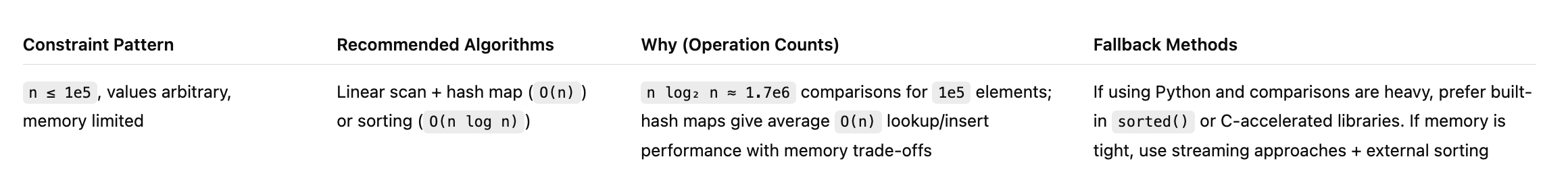
Concrete numeric example: decide between O(n log n) and O(n^2) for n ≤ 10^5 Estimate: n log2 n ≈ 10^5 · 17 = 1.7·10^6 comparisons; n^2 = 10^10 comparisons. Even with high per-comparison overhead, O(n log n) is feasible where O(n^2) is not. Ask whether output size or hidden constants change the calculus: if each comparison is expensive (e.g., long string comparisons) or required memory is large, further constraints may force alternative approaches.
Language and constant-factor trade-offs Asymptotic notation hides constants that matter in interviews and production. Python's per-loop and per-object costs are higher than C++; vectorized NumPy/PyTorch operations move work into native code with much smaller per-element overhead. When constraints sit near thresholds, prefer:
Implementations that use linear-time, low-allocation primitives (in-place edits, generators, iterators).
Offloading inner loops to native libraries (NumPy, C extensions) or using built-in sorting which is highly optimized (Timsort).
Document this reasoning aloud: "I could do an O(n log n) approach using sorting, but in Python I'll rely on sorted() because it's optimized; if data are huge I'll switch to streaming/partial aggregation to keep memory down."
Multi-dimensional and combined constraints Treat multi-parameter problems by identifying their independent axes. Examples:
Graphs: state complexity in terms of V and E. BFS/DFS on adjacency lists is O(V + E) time, O(V + E) memory; on adjacency matrix it is O(V^2) time and memory. For sparse graphs (E ≪ V^2), adjacency lists are almost always superior.
Parameterized problems: when complexity is O(k·n) or O(n·log k), make k explicit in feasibility checks. A solution with O(n·k) is acceptable if k ≤ 10^2; otherwise hunt for O(n log k) or O(n) variants.
ML: include sequence length n and hidden dimension d. Self-attention is O(n^2 d) time and O(n^2) memory for dense attention; if n grows (e.g., > 2k), dense attention often fails due to memory, motivating chunking or sparse approximations.
Output size and impossibility checks Always ask about required output size. If the problem demands enumerating all pairs that match a predicate, worst-case output may be Θ(n^2)—and no algorithm can avoid that cost. A correct interview answer explains that an O(n) algorithm is impossible when output size is quadratic and suggests returning counts or streaming matches instead.
Adversarial and worst-case inputs Hash-based structures (dict, unordered_map) provide average O(1) operations but can degrade under adversarial inputs causing collisions. In interviews and production, mention mitigations: use randomized hashing, stick to balanced-tree maps (O(log n) worst-case), or combine checks with input validation/timeouts. For production-facing code, prefer algorithms with predictable worst-case if inputs are untrusted.
A compact constraint-to-algorithm template Use a single template row to record your decision succinctly; fill this aloud when asked to choose an approach.
Practical interview phrasing and framing Sample spoken script to justify choice:
"What are n and any memory caps?" (clarify)
"Given n ≤ X, n log n is ≈ Y operations — that fits within expected limits; n^2 would be ≈ Z and is infeasible."
"If inputs are adversarial or memory-constrained, I'll use [fallback] because it provides predictable worst-case or lower memory."
Exercise (apply this immediately) Given n up to 10^5 and values up to 10^9: list the clarifying questions you'd ask, estimate operation counts for an O(n log n) sort versus O(n^2) nested loops, state whether you'd start with sorting/hash-map, and name one production mitigation if inputs are adversarial.
Failure modes and final cautions
Ignoring output size yields incorrect feasibility claims.
Treat average-case hash costs as conditional; mention collision mitigations.
Over-relying on asymptotics without numeric estimates invites poor choices near thresholds; always convert Big-O to concrete operation counts and cross-check with language/runtime characteristics.
For ML workloads, remember to include per-batch costs, activation memory, and optimizer state in memory budgets; sequence-length-driven quadratic costs are a common production bottleneck.
This checklist and template sharpen decisions under time pressure; an interviewer expects the reasoning path as much as the final complexity class.
Proof Patterns: Halving, Recurrences, and Comparison-Sort Intuition
Binary search and divide‑and‑conquer recurrences are the most interview‑useful proof patterns: halving (logarithms), recursion trees (levels × per‑level work), and the contrast with linear/unbalanced recurrences. Master these three compact templates and you can deliver tight, verbal complexity proofs that interviewers expect.
Halving (binary search): the halving argument is arithmetic and short. Start with n items. Each comparison reduces the search space by at least a factor of two; after k comparisons the remaining space is ≤ n / 2^k. The loop stops when n / 2^k ≤ 1, so 2^k ≥ n and k ≥ log2 n. Therefore binary search needs O(log n) comparisons. This is robust: whether you write an iterative loop or a tail‑recursive function, the number of iterations is bounded by ⌈log2 n⌉. Mention as you speak that the base of the logarithm is a constant and irrelevant for Big‑O.
Illustrative, interview‑ready binary search (loop invariant annotated — illustrative):
# illustrative binary search: returns index or -1
def binary_search(a: list[int], target: int) -> int:
    lo, hi = 0, len(a) - 1
    # invariant: target is in a[lo:hi+1] if present
    while lo <= hi:
        mid = (lo + hi) // 2
        v = a[mid]
        if v == target:
            return mid
        if v < target:
            lo = mid + 1  # preserve invariant
        else:
            hi = mid - 1  # preserve invariant
    return -1
# Time: O(log n) comparisons; Space: O(1)
Choose the invariant phrasing you can state concisely in an interview; that communicates correctness as well as complexity.
Recurrence intuition via recursion trees: for balanced divide‑and‑conquer recurrences of the form T(n) = a T(n/b) + f(n), the recursion‑tree picture clarifies growth. Each level of the tree contributes total work equal to the number of subproblems times the per‑subproblem nonrecursive work. Example: T(n) = 2 T(n/2) + Θ(n). Level 0 does Θ(n) work (the root). Level 1 has two subproblems of size n/2, so total Θ(2 · n/2) = Θ(n). Level 2 has 4 subproblems of size n/4; total Θ(4 · n/4) = Θ(n). This repeats for log2 n levels until subproblem size is constant. Summing Θ(n) per level over Θ(log n) levels yields Θ(n log n). In interview phrasing: "balanced split ⇒ Θ(n) per level × log n levels ⇒ Θ(n log n)."
Contrast with unbalanced splits and linear recurrences. T(n) = T(n−1) + Θ(1) is easy: the recursion tree is a chain of n levels with Θ(1) per level, giving Θ(n). The topology (chain vs. balanced tree) is the key driver. Always state the number of levels and the work per level when answering a recurrence question.
When to invoke the comparison‑sort lower bound: any comparison‑based sorting algorithm must perform Ω(n log n) comparisons in the worst case. The decision‑tree model argues there are n! possible input orderings and a binary comparison produces two branches, so a depth of at least log2(n!) = Ω(n log n) is required. Thus if your algorithm's dominant cost reduces to comparing arbitrary element orders, O(n log n) is not improvable with comparisons. In interviews, tie this to algorithm families: merge sort and heapsort achieve Θ(n log n) by balanced divide‑and‑conquer or heap operations; quicksort achieves Θ(n log n) average‑case but worst‑case Θ(n^2) under adversarial pivots.
Practical caveats and failure modes. Do not apply the balanced recurrence template if splits are not uniform or when f(n) dominates. For T(n) = 2 T(n/2) + n^2, per‑level work grows (level 0: n^2, level 1: 2·(n/2)^2 = n^2/2, ...), so the root dominates and T(n)=Θ(n^2). Always check which term dominates: the recursive tree may have either the root, the leaves, or all levels contributing equally. Common mistakes: treating a pointer‑movement double loop as O(n^2) without amortized reasoning (see next chapter), or blindly invoking the Master theorem when subproblems are uneven or when recursion depth is input‑dependent.
Interview phrasing templates (3–4 short sentences you can say aloud): state the recurrence, summarize per‑level work, state number of levels, sum and conclude. Example: "We have T(n)=2T(n/2)+Θ(n). Each level does Θ(n) work, there are Θ(log n) levels because size halves each time, so total is Θ(n log n)." Keep this under 30–40 seconds.
Production considerations: recursion depth matters in real systems. Implementations that recurse for Θ(log n) depth are fine; those that recurse O(n) depth (e.g., T(n)=T(n−1)+O(1)) risk stack overflows in languages without guaranteed tail‑call optimization (CPython). Convert to iterative forms when depth is large. Also remember constants and cache effects: Θ(n log n) with good locality (merge sort with sequential access) can outperform Θ(n log n) with poor locality (random memory accesses), so asymptotic class is necessary but not sufficient for engineering trade‑offs.
Connections to ML workloads: divide‑and‑conquer appears in hierarchical clustering and reductions over sequences; the same recursion‑tree intuition helps reason about algorithmic bottlenecks. Contrast hierarchical methods (Θ(n log n) or Θ(n log^2 n) depending on merges) with dense attention's Θ(n^2) cost — the cost per level and number of levels are directly analogous.
Short practice prompt to speak aloud: take T(n)=T(n−1)+O(1) and T(n)=2T(n/2)+O(n). For each, state levels, per‑level work, and final bound in one sentence. If you can do both in under 60 seconds, your verbal recurrence proofs are interview‑ready.
Amortized Analysis: Dynamic Arrays, Two-Pointer Patterns, Stacks, Heaps, and Union-Find
Amortized analysis answers the question: when an expensive operation occasionally appears in a repeated sequence, how should you account for its cost across the whole sequence rather than blaming a single outlier? Interviews expect a tight, repeatable argument: count relevant atomic actions across an entire sequence, bound that total by a simple function of N, and divide to get a per-operation amortized bound. The aggregate method is the most interview-friendly: add up actual costs over N operations and show the sum is O(N) (or whatever function), yielding O(1) amortized per operation when appropriate. Mention the potential or accounting method only when necessary: it provides a bookkeeping view that assigns "credits" to cheap operations to pay for later expensive ones, but the end result should match the aggregate count.
Dynamic arrays (geometric resizing). The classical dynamic array doubles capacity when full. A single append may trigger a resize costing O(k) copies where k is the current size; worst-case per-append is O(n). Aggregate analysis shows these copies sum to O(N) over N appends.
Illustrative pseudo‑Python for clarity (illustrative; production systems add preallocation and thread-safety):
class DynArray:
    def __init__(self):
        self.cap = 1
        self.buf = [None] * self.cap
        self.size = 0

    def append(self, x):
        if self.size == self.cap:
            # allocate new buffer of size 2*self.cap and copy
            new_cap = self.cap * 2
            new_buf = [None] * new_cap
            for i in range(self.size):   # cost: self.size copies
                new_buf[i] = self.buf[i]
            self.buf = new_buf
            self.cap = new_cap
        self.buf[self.size] = x
        self.size += 1
Why this yields amortized O(1). Let N be total appends. Every element gets copied at most once per resizing level; geometric capacities 1,2,4,... imply total copy work ≤ 2N. Summing k over resizes forms a geometric series bounded by 2N, so total work (copies + N actual writes) is O(N), thus amortized cost per append is O(1). Practical caveats: doubling uses up to ~2× peak memory; choosing a smaller factor (e.g., 1.5×) reduces memory overhead at the cost of more frequent, smaller resizes and a slightly larger constant in amortized cost. In latency-sensitive systems, amortized O(1) hides infrequent O(n) pauses; mitigations include preallocation, background/reserved resizing, or incremental copying to spread the cost across subsequent appends.
Two-pointer and sliding-window patterns. Many nested loops are not quadratic when the inner pointer only advances forward. The key observation: each pointer can increment at most N times. Count the pointer increments as atomic actions.
Concrete sliding-window example: find the longest subarray with sum ≤ S.
def max_subarray_len_at_most(nums, S):
    left = 0
    cur = 0
    best = 0
    for right, v in enumerate(nums):
        cur += v
        while cur > S:
            cur -= nums[left]
            left += 1
        best = max(best, right - left + 1)
    return best
Amortized argument: right increments N times in the for-loop; left increments only inside the while but can only move from 0 to N across the whole run, so total loop body executions are O(N). Therefore total time O(N). Interview phrasing to assert this: "Count the increments: right moves N times; left never moves backward, so at most N increments—thus the inner loop contributes at most N operations overall."
Union-Find: union by rank + path compression. Union-Find supports make-set, find, union such that an arbitrary sequence of M operations on N elements runs in nearly linear time. The formal amortized bound uses the inverse-Ackermann function α(N), which grows so slowly that for all practical N it is ≤ 4 or 5. Intuition: union by rank keeps trees shallow; path compression flattens trees during finds so future finds are cheaper. For interview purposes, state: with both heuristics, the amortized time per operation is α(N), so M operations cost O(M α(N)), effectively linear for realistic input sizes. If pressed, give the verbal sketch: each node's parent pointer moves closer to the root on compressions, and the number of times it can meaningfully move is extremely limited by the rank structure.
Heaps and stacks. Stacks have strict O(1) push/pop in worst-case. Binary heaps provide O(log n) push/pop worst-case; there is no amortization to improve push/pop asymptotics for binary heaps because each operation may require bubbling on the heap height. However, certain heap variants (e.g., Fibonacci heaps) provide amortized O(1) decrease-key and O(log n) delete-min; those are rarely used in coding interviews but useful to mention when algorithm choices hinge on many decrease-key operations (e.g., Dijkstra variants).
Hash tables. Average-case O(1) for lookups/inserts/deletes assumes a good hash and low load factor; worst-case can be O(n) under pathological collisions. Explain this explicitly: interviewers care that you know average vs worst-case, and when adversarial inputs matter (e.g., untrusted keys). Practical mitigations include using randomized hashes, changing hash seeds, or using tree-backed buckets (Python 3.7+ moves to trees above a bucket size threshold) to bound worst-case behavior.
Presenting amortized arguments succinctly (interview micro-script):
State the sequence and the expensive operation (resize, inner loop, find).
Count the atomic event across the whole sequence (copies, pointer increments, parent-pointer changes).
Sum the counts and bound them by a simple function of N (e.g., ≤ 2N); conclude amortized per-op cost.
This three-line structure maps cleanly to the aggregate method.
Failure modes and production trade-offs. Amortized guarantees are about long-run averages, not tail latency. Systems that require tight p99 latency must avoid occasional O(n) spikes or hide them—pre-warm buffers, perform background resizing, or batch operations differently. Memory overhead from over-provisioning (doubling) interacts with memory-constrained environments and GC behavior in managed languages; prefer explicit capacity hints or pooling. In ML systems, similar amortized reasoning applies: KV caches for autoregressive decoding make each new token cheap amortized across sequence generation, but the first inference involving big cache construction may be heavy—plan for warm-up or streaming strategies.
Exercises to practice: write one-paragraph amortized proofs for (1) dynamic array doubling, (2) the two-pointer sliding-window algorithm above, and (3) Union-Find with union-by-rank plus path compression. Time yourself: deliver each proof in 30–60 seconds aloud, using the three-line micro-script. Assess each proof on clarity of counted events, correctness of bounds, and identification of practical caveats (memory, latency spikes, adversarial inputs).
Space Complexity: Stack, Output, Auxiliary Memory, and In-place Mutation
Space complexity is not a single number; it is a taxonomy you must enumerate when you state an algorithm’s memory usage. Every interviewable complexity statement should account for four distinct components: the recursion/activation stack, the size of the output the algorithm must produce, auxiliary (working) memory used by the algorithm, and transient temporary buffers produced by language or library primitives. Omitting any of these leads to incorrect or misleading claims—especially when outputs are large (e.g., returning all pairs) or when language primitives hide copies (Python slicing, string concatenation).
Recursion stack and activation frames Recursive calls allocate stack frames proportional to recursion depth. Each frame contains local variables, return address, and language/runtime bookkeeping; account for this as O(d) where d is maximum depth. In a chain-like graph (a path) with V nodes, a naive recursive DFS allocates O(V) stack frames; in CPython this can trigger RecursionError when V exceeds the interpreter limit (≈1000 by default). Tail-call elimination is not available in CPython, so do not assume tail recursion reduces stack usage. If d may be large or unbounded, transform to an iterative algorithm that explicitly manages a stack on the heap or use an explicit loop.
Illustrative example — recursive DFS vs iterative DFS (Python, illustrative) The recursive version is compact but uses O(d) call-stack memory. The iterative version replaces implicit stack frames with an explicit list, making stack memory explicit and under program control (and avoiding interpreter recursion limits). Comments annotate space costs.
# Illustrative: recursive DFS (stack implicit)
def dfs_recursive(adj, start, visited=None):
    if visited is None:
        visited = set()
    visited.add(start)
    for nbr in adj[start]:
        if nbr not in visited:
            dfs_recursive(adj, nbr, visited)
    return visited  # visited size O(V)

# Space: recursion stack O(d) (d = depth), visited set O(V).
# On a chain graph d = V -> call stack O(V) (can overflow CPython recursion limit).
# Illustrative: iterative DFS (stack explicit)
def dfs_iterative(adj, start):
visited = set()
stack = [start] # explicit stack; size O(d) worst-case
while stack:
node = stack.pop()
if node in visited:
continue
visited.add(node)
for nbr in adj[node]:
if nbr not in visited:
stack.append(nbr)
return visited
# Space: explicit stack O(d), visited set O(V).
# Iterative version avoids interpreter recursion limits; memory accounting is explicit.Output size must be counted If an algorithm returns a collection of results, that output is part of the space complexity. Returning all pairs from n items creates Θ(n^2) output. Even if the algorithm internally used only O(1) auxiliary memory, the total memory required is dominated by output: returning all pairs forces O(n^2) memory and potentially O(n^2) time to construct. Many interviewers test for this trap: "If I ask you to return all pairs, how does that change your memory claims?" Answer: include O(k) where k is the number of outputs; if k = Θ(n^2), space is Θ(n^2).
Streaming vs materializing When outputs are large, streaming (generators, iterators) avoids materializing the whole result. This shifts memory from O(k) to O(1) (plus any buffer). Streaming introduces API/semantic trade-offs: callers must consume the generator, error handling and retries are more complex, and parallel/async consumption requires additional coordination. In production, streaming is often the only viable option for very large k.
Example — all-pairs materialized vs generator (Python, illustrative)
# Materialize all pairs: O(n^2) memory and time to build list
def all_pairs_list(arr):
    out = []
    n = len(arr)
    for i in range(n):
        for j in range(i+1, n):
            out.append((arr[i], arr[j]))
    return out  # memory O(n^2)

# Generator: O(1) auxiliary memory, same total time to iterate all elements
def all_pairs_gen(arr):
    n = len(arr)
    for i in range(n):
        for j in range(i+1, n):
            yield (arr[i], arr[j])
State the trade-offs: materialized list is simpler for random access and re-iteration; generator is memory-efficient but single-pass and requires caller cooperation.
Auxiliary memory and temporary buffers Auxiliary memory includes data-structures you create in addition to the output and stack (hash tables, temporary arrays, priority queues). Temporary buffers are frequently introduced implicitly by language primitives: list slicing produces copies (O(k) memory), string concatenation in a loop produces repeated allocation cost unless done via join, and sorted() returns a new list. In interviews, explicitly call out when an operation performs copying and quantify its cost.
In-place mutation vs copying: correctness, testing, and failure modes In-place mutation reduces auxiliary memory but changes the function’s semantics: it can surprise callers, complicate reasoning about aliasing, and create harder-to-test code. For example, reversing a list in-place is O(1) auxiliary memory; returning a new reversed list is O(n). When you propose in-place approaches in interviews, justify them: are inputs allowed to be mutated? Are there concurrency or rollback requirements? In production, if immutability is required (for safety or reproducibility), copying may be the only correct choice despite the memory cost.
Concrete example — reverse in-place vs copy
def reverse_inplace(a):
    i, j = 0, len(a)-1
    while i < j:
        a[i], a[j] = a[j], a[i]
        i += 1
        j -= 1
    return a  # O(1) aux; original list mutated

def reverse_copy(a):
    return a[::-1]  # O(n) memory for the returned list; original preserved
Note that a[::-1] creates a new list via slicing; document that cost, and prefer list(reversed(a)) if you want clarity in intent.
Recursion-to-iteration transforms and patterns When depth is a concern, common transforms include: explicit stack simulation (generic), converting tail recursion into a loop (if semantics allow), or reformulating the algorithm into an iterative dynamic programming solution where the data-dependency graph is acyclic and traversal order can be arranged bottom-up. For languages with small recursion limits, prefer iterative transforms for production reliability.
ML-system analogy: activations and optimizer state are memory outputs In ML training, treat activations and optimizer accumulators like outputs or auxiliary buffers. A model with sequence length n and hidden dimension d may consume O(n·d) activation memory per layer, and self-attention additionally incurs O(n^2) memory for attention scores. When enumerating space for a training step, list activations, parameters, optimizer states, and any cached K/V tensors; quantify each term in Big-O and note batch size and sequence length multiplicative effects. This mirrors the output/aux distinction: activations are required for backward and therefore must be counted even if they are transient.
Failure modes and pragmatic rules
Forgetting to include the output: proposing O(1) auxiliary memory while returning Θ(n^2) results is a common error. Always add O(k) for k results.
Assuming tail-call elimination in Python: explicitly warn that CPython lacks TCO and that recursion depth can cause runtime failure.
Underestimating hidden copies: slicing, concatenation, and some library routines copy memory. When memory is tight, prefer in-place or streaming primitives and measure empirically.
Mutating inputs in libraries or multithreaded contexts can produce elusive bugs; document mutation semantics and add tests that assert original input unchanged when required.
How to present memory accounting concisely in interviews State the taxonomy, then quantify each term. A concise script:
"Space = recursion/stack O(d) + output O(k) + auxiliary O(a)."
"In this problem k is (e.g., number of pairs) = Θ(n^2), so total space Θ(n^2)."
"If memory is tight, I can stream results via a generator or convert recursion to an iterative stack to avoid interpreter recursion limits; in-place mutation saves memory but changes semantics—ask whether mutation is allowed."
Quick checklist to apply when reasoning:
Identify output size k and include O(k).
Bound recursion depth d; include O(d) for stack.
List auxiliary structures with their sizes (hash maps, heaps, arrays).
Call out language-level copies (slicing, join, sorted) and factor them in.
State mutation semantics and concurrency implications.
Practicing these steps on common interview problems (e.g., DFS on chains, all-pairs generation, in-place array transforms) converts surface-level Big-O claims into defensible, interview-ready statements.
Hash Tables, Collision Behavior, and Classic Interview Examples (Two Sum, Anagram, Contains Duplicate)
Hash tables give algorithm designers practical O(1) lookup and insert in everyday code, but the phrase "dict is O(1)" is shorthand that must be qualified in both interviews and production design. The average-case O(1) bound holds under two assumptions: a good hash function that distributes keys uniformly across buckets, and a bounded load factor so that the expected bucket occupancy remains constant. When either assumption fails—due to poor hashing, adversarial inputs that collide, or aggressive load factors—an operation's cost can degrade toward O(n). Interviews probe both the efficient path and the pathological caveats; production systems must mitigate the pathological cases.
Why average is O(1). A chained hash table with m buckets and n keys has expected bucket length n/m, the load factor α. If the hash function assigns keys uniformly, the expected time to examine one bucket is proportional to 1 + α. Resizing strategies keep α bounded (e.g., α ≤ 1 or ≤ 0.75), so expected cost per operation is constant. Open-addressing schemes (linear probing, quadratic, robin-hood) trade bucket occupancy patterns for cache locality; they still rely on bounded α for constant expected probes.
Why worst-case is O(n). An adversary who can choose keys that collide will force all keys into a single bucket for chaining, or into long probe sequences for open addressing. In that case, operations require scanning O(n) items. Real-world services exposed to untrusted inputs must assume this risk. Two practical mitigations are randomized hashing (per-process or per-request random seeds) and limiting work per request (size limits, timeouts, or circuit-breaking).
Production mitigations and trade-offs. Randomized hash seeds reduce the ability of an attacker to craft collisions, turning adversarial inputs into probabilistic failures rather than deterministic exploits. Randomization is low-cost but complicates reproducibility: salted hashes in a server should be stable for a request's lifetime but rotated if you want per-worker randomness. Load-factor tuning and incremental resizing keep probe costs low at the expense of higher memory overhead. For extreme scale or adversarial settings, use fallback structures (balanced trees or sorted arrays) with guaranteed logarithmic or linear bounds. Finally, rate-limit input sizes and enforce quotas before allocating proportional memory to requests.
Two Sum: baseline and optimal hash approach. Classic prompt: given array nums and target, return indices i, j with nums[i] + nums[j] == target. Baseline: sort with indices retained, then two-pointer search at O(n log n) time and O(n) auxiliary space for index bookkeeping. Optimal interview answer uses a single-pass hash map. Key pitfalls: avoid inserting the current element before checking, or you'll pair an element with itself incorrectly; state average versus worst-case behavior of the map and propose mitigations.
Illustrative: Two Sum (Python, interview-ready, illustrative)
# Illustrative example: Two Sum (returns indices)
# Average-case: O(n) time, O(n) extra space. Worst-case (hash collisions): O(n^2) if every lookup degenerates.
def two_sum(nums, target):
    seen = {}  # value -> index
    for i, x in enumerate(nums):
        y = target - x
        if y in seen:          # average O(1) lookup; worst-case O(n)
            return [seen[y], i]
        seen[x] = i            # average O(1) insert
    return None
Why this code is written this way: checking for the complement before inserting prevents the same element from being reused; storing index on first sight retains the earliest index which matches many prompt expectations. Complexity proof sketch: one pass of n iterations, each contains O(1) expected work for a lookup and possibly an insert → O(n) expected time. Space stores at most n entries → O(n) space. Adversarial collisions convert each lookup/insert into O(n) scanning of a bucket; repeated for n iterations gives O(n^2) worst-case.
Valid Anagram: counting vs sorting. For fixed small alphabets (e.g., lowercase English), counting with a fixed-size array is O(n) time and O(k) auxiliary space where k is alphabet size (26). For Unicode or unknown alphabet, use a hash map Counter (average O(n) time, O(k) space) or sort both strings (O(n log n) time, O(1) extra space if in-place). Unicode forces two considerations: the alphabet size may be large, so k can be comparable to n; normalization (NFC/NFD) must be applied before counting, or character-level counts may differ.
Illustrative: Valid Anagram (ASCII lowercase optimization)
# Illustrative example: Valid Anagram for lowercase ASCII
# Time: O(n), Space: O(1) auxiliary (26 counters)
def is_anagram(a, b):
    if len(a) != len(b):
        return False
    counts = [0] * 26
    base = ord('a')
    for ch in a:
        counts[ord(ch) - base] += 1
    for ch in b:
        counts[ord(ch) - base] -= 1
    return all(c == 0 for c in counts)
When to choose each method: use counting for small or known alphabets, Counter/dict for general Unicode sets (noting average-case hash costs), and sorting when memory is very constrained or when you can mutate in-place and accept O(n log n) time.
Contains Duplicate: set-based detection and alternatives. Using a set to detect duplicates in one pass is average O(n) time and O(n) space. If memory is constrained or worst-case guarantees are required, sort in-place and check adjacent neighbors in O(n log n) time and O(1) extra space. For streaming inputs where you cannot store all elements, use probabilistic structures (Bloom filters) to get memory-limited approximate answers with tunable false-positive rates.
What to say in an interview. A concise spoken structure makes the difference:
Assumptions: clarify input size n, whether keys are adversarial, alphabet constraints, memory limits.
Algorithm sketch: single-pass hash with complement check (for Two Sum); counting array vs Counter vs sort (for anagram).
Complexity: state expected/worst-case time and space and the assumptions behind the averages.
Edge cases and mitigations: same-index reuse, Unicode normalization, hash-seed randomization, fallbacks (sorted approach, rate limiting).
Failure modes to call out. Failing to mention worst-case hash behavior or to handle duplicate/index semantics are frequent interview deductions. In production, unbounded memory allocation from per-request hash tables leads to DoS. Randomized hashing plus request-size caps and quotas is the practical engineering pattern: preserve average-case performance while bounding worst-case resource consumption.
Practice prompt. Deliver a one-paragraph proof for Two Sum aloud: state assumptions (uniform hashing or randomized seed), sketch the single-pass algorithm and its O(n) expected time, O(n) space, then append the worst-case O(n^2) caveat under pathological collisions and two mitigations: randomize hash seeds and enforce input-size limits. This compact script becomes the reliable interview answer that balances algorithmic correctness with production-savvy nuance.
Graph Representations and BFS/DFS Complexity: Sparse vs Dense Trade-offs
Representing a graph is a design decision with immediate asymptotic and practical consequences. The same algorithm—BFS or DFS—has two common complexity narratives depending on representation: with an adjacency list you reason in terms of vertices V and edges E, giving O(V + E) time; with an adjacency matrix you trade iteration cost for constant-time edge membership tests, giving O(V^2) time but O(1) checks for edge existence. Interviews expect not only the O(·) statements but the counting argument and the representation decision driven by E relative to V^2, memory budget, and the common operations the algorithm must perform.
Why BFS is O(V + E) with an adjacency list BFS enqueues each vertex at most once and dequeues it at most once. Visiting a dequeued vertex v requires iterating over v’s adjacency list; the total number of adjacency-list entries visited across the entire run equals E (directed) or 2E (undirected counted per direction). Thus the work breaks down into at most O(V) for queue and visited bookkeeping plus O(E) for scanning neighbor lists, giving O(V + E) total time. The auxiliary space is O(V) for the visited set and the queue; the adjacency list itself costs O(V + E) memory to store.
Annotated, interview-friendly BFS (illustrative) This is a compact, idiomatic Python implementation emphasizing the representation and complexity annotations. It is illustrative—use adjacency lists for sparse graphs.
from collections import deque, defaultdict
from typing import Dict, List, Iterable

def bfs(start: int, adj: Dict[int, List[int]]) -> Iterable[int]:
    """
    Breadth-first traversal yielding nodes in BFS order.

    Complexity (adjacency list): Time O(V + E), Space O(V) extra.
    - Each vertex enqueued/dequeued once -> O(V)
    - Each adjacency entry visited once -> O(E)
    """
    seen = set([start])            # O(1) average per membership insert
    q = deque([start])             # queue operations O(1)
    while q:
        u = q.popleft()
        yield u
        for v in adj.get(u, []):   # iterating neighbors accounts for E over whole run
            if v not in seen:
                seen.add(v)
                q.append(v)
Important implementation choices: use deque for O(1) queue ops; keep visited as a hash set for average O(1) membership; store adjacency lists as lists (or arrays) for efficient iteration, not as sets—iteration cost is what we count into E.
Adjacency matrix: when and why it matters An adjacency matrix is a V×V boolean (or bit) matrix. Time to run BFS by scanning a row for neighbors is O(V) per vertex, giving O(V^2) time overall; memory is O(V^2). Where an adjacency matrix shines:
Dense graphs where E ≈ V^2: O(V^2) time and O(V^2) memory may be acceptable, and iteration over rows is straightforward and cache-friendly for small V.
Algorithms that require frequent edge-existence queries between arbitrary pairs perform better: matrix offers O(1) edge checks versus an adjacency list’s expected O(deg(u)) cost when scanning or O(1) average for hash-based neighbor sets but with extra storage and hash overhead.
Bit-packed matrices reduce memory constant factors and enable word-level parallelism.
But for large V and sparse E, matrix memory is prohibitive. Example: V = 100,000 gives V^2 = 10^10 entries; even a bit per entry would require gigabytes beyond realistic RAM.
Counting and practical numeric comparisons
Sparse scenario: V = 100,000, E ≈ 200,000. Adjacency list memory ≈ O(V + E) ~ 300k entries (feasible); adjacency matrix ~ 10^10 entries (impossible).
Dense small graph: V = 1,000, E ≈ 500k. Matrix memory ~ 1e6 entries—feasible—and row scans may outperform random memory accesses for lists due to contiguous memory and lower pointer overhead.
Complete graph: E = V(V − 1)/2 ≈ V^2/2. BFS time is O(V + E) = O(V^2). Using matrix representation yields the same asymptotic time but simplifies coding and edge checks.
Directed graphs, multigraphs, and edge semantics Always clarify whether the graph is directed or undirected. For directed graphs, the E in O(V + E) is the number of directed edges; for undirected graphs count each undirected edge as a single edge but realize the adjacency list stores it twice (once per endpoint), which affects memory constants and edge-visit counting (often resulting in 2E neighbor entries scanned). Multigraphs and parallel edges increase E directly and must be included in complexity counts.
When edge-existence checks change the asymptotic story High-level algorithms sometimes perform many arbitrary edge queries (e.g., algorithms that require checking whether two vertices are connected by an edge repeatedly, not just iterating neighbors). For such algorithms, matrix O(1) checks can reduce higher-level complexity—from O(k × deg(u)) to O(k) for k queries—altering algorithmic choices. Conversely, if the algorithm spends its time enumerating neighbors, adjacency lists win.
Memory formats for very large graphs For large sparse graphs stored on disk or in ML pipelines, use compressed sparse row (CSR) or compressed sparse column (CSC) formats: neighbor lists packed into contiguous arrays with index pointers per vertex. CSR reduces memory overhead compared to pointer-based lists and improves cache behavior for neighbor iteration—useful for graph neural networks and minibatch sampling. External-memory or streaming representations exist, but they introduce new complexity: I/O bandwidth, partitioning, and consistency when mutating graphs.
Python pitfalls and production caveats Python adjacency lists using lists of ints are convenient but carry per-object overhead (pointer-rich lists, boxed integers) and can blow memory constants compared to compact C arrays. For very large graphs, use numpy arrays for neighbor storage or frameworks (SparseCSR from scipy, graph-tool, or custom C++ backends). Hash-based neighbor sets permit O(1) average membership checks but increase memory and hurt iteration speed.
Failure modes and algorithmic anti-patterns
Choosing a matrix for large sparse graphs leads to immediate memory exhaustion.
Assuming adjacency-list iteration is cheap without accounting for skewed degree distributions: a small set of high-degree vertices can dominate runtime.
Neglecting the cost of edge duplication in undirected adjacency lists when counting memory.
Using Python lists and sets for production-sized graphs without benchmarking memory and traversal throughput.
Interview phrasing to elicit necessary constraints Ask: Is the graph directed or undirected? What are typical V and E (or a relationship between them)? Are we optimizing for neighbor iteration or for arbitrary edge-existence queries? What are memory limits? These clarifying questions let you state O(V + E) for adjacency lists and O(V^2) for matrices and then recommend representation succinctly.
Practical decision heuristic Estimate V and E. If E ≪ V^2 (sparse), use adjacency lists/CSR: time O(V + E), memory O(V + E). If E ≈ V^2 and V is small enough to allocate V^2 entries, adjacency matrix simplifies logic and supports O(1) edge queries. Consider intermediate choices (bit-packed matrices, CSR, or hybrid representations) when memory constants, cache locality, or frequent edge-existence checks influence performance.
Exercise (mental): For a complete graph with V = 10,000, compute the memory for an adjacency matrix of booleans and recommend representation. Enumerate whether BFS/DFS complexity changes in practice and why an adjacency list is still logically O(V + E) = O(V^2) but disastrous in memory for this V without compact storage.
ML-Specific Complexity: Transformer Self-Attention, Activations, Optimizer State, and KV Cache
Derive the per-layer arithmetic and memory cost of dense self-attention in concrete terms: queries Q, keys K, and values V are produced by projecting the input X of shape (B, n, d) into h heads of dimension dh (so d = h * dh). For a single head the core attention score is S = Q · K^T, an (n × n) matrix per example. Computing S requires roughly 2 · n^2 · dh floating-point multiply-adds (one multiply and one add counted as two fused ops is a common accounting; constant factors matter for runtime but not asymptotics). Applying attention to values multiplies the softmaxed S by V, another O(n^2 · dh). Aggregating across heads and batch gives the standard asymptotic time:
Time per layer ≈ O(B · h · n^2 · dh) = O(B · n^2 · d).
Memory pressure is dominated by materialized attention scores and activations. Storing the score matrix S for all heads and batch requires B · h · n^2 floats, so memory scales as O(B · h · n^2) = O(B · n^2) (up to the head-splitting constant). Activations after the attention (the output tensors) and intermediate projectors contribute O(B · n · d) each. Optimizers and training bookkeeping add further multiplicative constants: Adam-style optimizers typically store two additional tensors per model parameter (first and second moment), so parameter-state memory ≈ 3 × model_params for float32 Adam. KV caches used in autoregressive decoding grow linearly with sequence length: a cache sized O(B · n · d) if keys/values are stored per token.
Concrete arithmetic clarifies why “quadratic in n” is a practical showstopper. Assume float32 = 4 bytes per value. For B = 16, n = 2048, d = 1024, h = 16 (dh = 64):
Attention scores memory: B · h · n^2 · 4 bytes = 16 · 16 · 2048^2 · 4 ≈ 16 · 16 · 4,194,304 · 4 ≈ 4.29e9 bytes ≈ 4.0 GiB just to hold S (and that’s per layer; many implementations materialize S for backward).
Activations (layer outputs): B · n · d · 4 = 16 · 2048 · 1024 · 4 ≈ 134,217,728 bytes ≈ 128 MiB.
Optimizer state (for model params) and intermediate projections easily add tens of GiB for large models.
This arithmetic demonstrates two practical truths: (1) materializing full attention scores across heads and batch imminently exhausts GPU memory at moderate n; (2) the quadratic term dominates memory even when d is large, because n^2 grows faster than n·d for typical regimes where n is large.
Mitigations and their asymptotic effects
Chunked/local attention: Restrict attention to fixed-size windows of size w (per-token receptive field). Compute attention within each window or between neighboring windows. Time and memory reduce from O(n^2) to O(n · w) per head: O(B · h · n · w · dh) time and O(B · h · n · w) memory. This is linear in n when w is constant. Trade-offs: receptive-field truncation impairs long-range interactions; overlapping windows or dilated patterns partially recover context at increased work.
Sparse / locality-sensitive hashing (LSH) attention: Use sparsity patterns or hashing to compute only top-k key matches per query. If each query attends to r keys on average, time becomes O(B · h · n · r · dh) and memory O(B · h · n · r). If r ≪ n, this is sub-quadratic. Trade-offs: hashing induces approximation error, can be sensitive to distribution shift, and worst-case adversarial inputs could force r→n unless mitigated.
Low-rank / linearized attention: Approximate K and V interactions by projecting into a low-rank basis (rank r), so that S ≈ Q · (K'ˆT) with K' of reduced rank. Complexity drops to O(B · h · n · r · dh) or O(B · n · d · r/dh) depending on formulation. Trade-offs: introduces approximation error proportional to how well cross-token covariance is low-rank; requires careful tuning of r and sometimes additional regularization.
Gradient checkpointing / recomputation: Reduce activation memory by not storing certain intermediate activations during forward pass, recomputing them during backward. Memory for activations can be reduced from O(B · n · d) to a fraction thereof at the cost of extra forward computation: time increases (often by a constant factor) while peak memory drops. This is an engineering lever when compute is cheaper than memory.
Mixed precision and sharding: Using float16 or bfloat16 halves memory for activations and attention scores (with numerical-stability caveats such as reduced dynamic range). Parameter and optimizer sharding across devices (e.g., ZeRO-style partitioning) spreads optimizer state and activations across multiple GPUs, turning per-device OOM into a global-capacity problem. Asymptotically these do not change n dependence; they reduce constant factors and change practical feasibility boundaries.
KV cache considerations for decoding
KV cache memory grows O(B · n · d) because for autoregressive decoding each generated token appends K and V vectors to the cache. For very long autoregressive sequences this linear growth dominates if attention is computed over the entire cache. Combining KV caching with sparse attention, chunking, or windowed decoding reduces the effective attention length and peak memory. When the model attends to the full cache, time per decode step may also be O(n · d) leading to quadratic cumulative decoding work over sequence length if each step attends to all previous tokens; design choices (e.g., caching precomputed key/value matrix products) can mitigate repeated recomputation.
Presentation for interviews — concise script template (≈90s)
Start: "Dense self-attention computes Q·K^T giving an n-by-n score per head; with batch B and h heads the time per layer is O(B·h·n^2·dh) or equivalently O(B·n^2·d), and memory to store scores is O(B·n^2)." Break down: "Activations cost O(B·n·d); optimizer states add roughly 2× parameters for Adam; KV cache grows O(B·n·d) during autoregressive decoding." Mitigation: "Common fixes—chunked/local attention reduces n^2 to n·w; sparse/LSH or low-rank attention make it roughly O(n·r) where r ≪ n; gradient checkpointing trades compute for memory; mixed precision halves constants. Each mitigation reduces asymptotic or constant costs at the expense of approximation error, reduced receptive field, or extra compute and implementation complexity." Close: "Choose mitigation based on acceptable error, target hardware (memory vs compute balance), and whether long-range exact attention is required."
Illustrative arithmetic snippet (labelled illustrative)
# Illustrative: compute attention memory/time estimates (floats => 4 bytes)
def attention_budget(B, n, d, h, dtype_bytes=4):
    dh = d // h
    score_mem = B * h * n * n * dtype_bytes
    activ_mem = B * n * d * dtype_bytes
    time_ops = 2 * B * h * n * n * dh  # rough multiply-add count for QK and S*V
    return dict(score_mem=score_mem, activ_mem=activ_mem, time_ops=time_ops)

# Example
print(attention_budget(B=16, n=2048, d=1024, h=16))
This arithmetic snippet emphasizes assumptions: dtype size, head split, and that backward passes can double peak activations. In production, always compute per-device budgets (not global) and include optimizer state and reserved GPU memory. Failure modes to call out: materializing full S in backward causes OOM; approximations can break when long-range dependencies are critical; hash-based sparsity can be adversarially manipulated or fail on out-of-distribution sequences. When discussing complexity in interviews or design reviews, pair the asymptotic statement with one numeric example and a clear mitigation choice tied to task fidelity and hardware constraints.
Hidden Costs in Python: Slicing, Concatenation, Membership, Sorting, and Heaps
High-level Python operations hide allocation and traversal costs that routinely flip an algorithm’s asymptotic behavior. A loop that looks linear at the source level can become quadratic because of repeated copying; string operations, slicing, membership checks, and certain container methods carry non‑obvious per‑operation costs. Interview answers that simply state “this is O(n)” without naming these hidden costs will be judged incomplete. Articulate the actual dominating operations — copying, hashing, shifting elements — and prefer idiomatic, C-implemented primitives or alternative data structures when performance matters.
Why copying matters: slicing and immutable concatenation Slicing a list or string produces a new object and copies the slice’s elements. The time cost is proportional to the slice length, not constant. If you repeatedly slice inside a loop, those per‑iteration copy costs accumulate. The common anti‑pattern is:
Illustrative: repeated slicing (inefficient)
# Illustrative example: inefficient due to repeated copying
def pop_front_naive(arr):
    result = []
    while arr:
        result.append(arr[0])   # O(1) to index
        arr = arr[1:]           # O(k) copy of k=len(arr)-1 -> quadratic overall
    return result
That code is O(n^2) time and O(n) peak extra memory because each arr[1:] allocates a new list of shrinking size. The correct mental model is: slicing cost = O(k) where k is slice length. To fix, avoid copying by using indices or a deque:
Idiomatic alternatives
from collections import deque

def pop_front_deque(arr):
    dq = deque(arr)           # O(n) one-time cost to build
    result = []
    while dq:
        result.append(dq.popleft())  # O(1) amortized
    return result
Deque popleft is amortized O(1); converting once to deque pays a linear one-time cost and removes the quadratic copying.
String concatenation: join versus repeated + Strings are immutable; s += t repeatedly constructs new strings and copies content each time. Repeated concatenation in a loop becomes O(n^2) where n is total characters. The correct idiom is to collect fragments and join once:
Illustrative: join vs repeated concatenation microbenchmark
# Illustrative microbenchmark: use time.perf_counter and repeats
import timeit

setup = "fragments = ['x'] * 10000"
stmt_plus = "s='';\nfor x in fragments:\n    s += x"
stmt_join = "s = ''.join(fragments)"

def run(stmt):
    t = timeit.timeit(stmt, setup=setup, number=10)
    return t

print("plus:", run(stmt_plus))
print("join:", run(stmt_join))
Warm-up and multiple trials matter; report medians. For large N, join is O(total_chars) and repeated + is O(n^2).
Membership checks and the right container choice "if x in list" is linear O(n); "if x in set" or dict lookup is average-case O(1) (amortized), with worst-case O(n) under hash-collision attacks or degenerate hash functions. For interview answers, state average vs worst-case and mitigation (use randomized hashing/seeding, validate adversarial input assumptions). When alphabet size is small and dense (e.g., ASCII letters), counting via array (list of size 26) is faster and avoids hashing overhead compared to Counter.
Counter, defaultdict, and small-alphabet trade-offs collections.Counter is convenient but wraps a dict and has per-key overhead. For tight loops over a small bounded alphabet, a preallocated list or numpy array has lower constant factors and memory. Use Counter when keys are many or unknown; prefer array counters when domain is fixed and dense.
Sorting and heap operations: expected costs and use-cases sorted() and list.sort() are Timsort: O(n log n) worst-case, but with excellent constant factors and adaptivity for partially sorted data. heapq.heappush/pop are O(log n) each and are appropriate when you need repeated min/max retrieval with interleaved insertions. For selecting k smallest elements from n, consider heap of size k (O(n log k)) or use heapq.nsmallest which internally selects the best algorithm based on k.
List append vs insert/pop(0) list.append is amortized O(1). insert(0, x) and pop(0) are O(n) because they shift elements. The amortized argument for append relies on geometric resizing: growing capacity by constant factors makes the average cost per append constant even though occasional resizes are O(n).
Heaps and amortized behavior Python’s heapq is a simple binary heap over a list; push and pop are O(log n). Building a heap from an array is O(n) with heapify (Floyd’s algorithm) — an important optimization when you need to heapify once rather than push n times.
Practical microbenchmarking: rules for trustworthy timings Microbenchmarks are useful to validate asymptotic reasoning and to expose constant‑factor differences. Follow these rules: warm up the interpreter, run multiple trials, report median and variance, and test on representative input sizes (include large N where asymptotics dominate). Use timeit or perf for reliable measurement. When benchmarking Python vs NumPy/PyTorch alternatives, ensure that heavy computations are actually performed in C (vectorized) to avoid Python loop overhead.
Production implications and when to prefer native libraries For compute-heavy workloads or large N, prefer C-implemented primitives or vectorized libraries. Example: accumulating gradients or large-array operations belong in NumPy/PyTorch; avoid Python-level elementwise loops. When memory is constrained, prefer in-place operations and be explicit about copies (e.g., arr.copy()) to avoid surprises.
Common failure modes to call out in interviews
Assuming average-case hash table complexity without noting worst-case adversarial inputs.
Saying "slicing is O(1)" — slices copy.
Using repeated string concatenation in a loop.
Using list.pop(0) or insert(0, …) in long-running loops.
Building a heap by n heappush calls instead of heapify when initial data exists.
Cheat-sheet template and exercise guidance For exch0033, produce one page entries with this pattern: operation → typical complexity (avg/worst) → minimal example → caveat → recommended idiom. Include entries for: list.append, list.pop(0), slicing, string + vs join, 'in' for list/set/dict, dict/set avg vs worst-case, Counter, sorted(), heapq.* and deque operations. As part of the exercise, include a short microbenchmark for the most surprising items (concat, slicing, pop(0)) using the timing rules above and summarize results with a short note on when to prefer the idiom in production.
How to say it succinctly in an interview Ask: “What are acceptable input sizes and adversarial assumptions?” Then point out specific hidden costs in the provided code (slicing copies, repeated concatenation, linear membership). Propose the idiomic fix and state the new asymptotic cost and memory footprint. That concise pattern — identify hidden allocation, present an O(n) or O(1) alternative, and quantify memory — is what interviewers expect.
Microbenchmarks, Empirical Validation, and Benchmarking Methodology
Empirical validation converts asymptotic claims from the chalkboard into measurable facts. A reproducible microbenchmark must answer three questions reliably: does the runtime grow as claimed; what are the dominating constants; and what hidden system factors could invalidate the measurement in production? The pattern that produces defensible answers is: warm the environment, run multiple independent trials per input size, measure both time and memory, fit a slope on log-log axes to infer the growth exponent, and record full hardware and software context so results are reproducible and interpretable.
Warm-up and determinism First iterations are polluted by cold-start costs: OS page faults, allocator buckets, Python interpreter startup, JIT compilation (PyPy, Numba, Torch JIT), and CPU turbo or frequency scaling. Execute a deterministic warm-up phase that exercises the same code paths and data shapes you will measure. Use fixed random seeds for synthetic data; prefer representative distributions over purely uniform randomness when benchmarking real workloads. Warm-up should run until measured time stabilizes, typically 5–20 iterations for small kernels, but verify by observing a plateau.
Multi-trial statistics Do not report single-run times. Run T independent trials (T >= 5) for each input size n and report the median and an interquartile range. Median is robust against transient OS noise and background processes. Keep trials independent: re-create inputs for each trial to exercise allocation behavior and avoid in-memory cache artifacts unless you intend to measure cache benefits.
Log-log slope estimation The asymptotic exponent k in O(n^k) is estimated by fitting a line to (log n, log time). Use only the input range where the runtime is well above measurement noise and not saturated by memory bandwidth or GPU out-of-core behavior. Fit using ordinary least squares on log-transformed median times; the fitted slope approximates k. Deviations of the slope indicate either a different asymptotic class or a transition between regimes (e.g., CPU-bound vs memory-bound). Always show both raw tables and the log-log plot.
Measuring memory Peak memory can be the limiting resource even when time appears acceptable. On CPU, use tracemalloc for Python-level allocations and psutil.Process().memoryinfo().rss for resident set size. On GPU, use framework APIs: torch.cuda.resetpeakmemorystats(); torch.cuda.maxmemoryallocated(). Record both peak and steady-state allocations. Memory measurement must be performed in-process to avoid sampling errors and to capture allocator fragmentation.
Isolating compute vs IO Separate data-loading from compute. For ML kernels, test synthetic tensors (random inputs of correct shape) to profile compute kernels and separately measure data pipeline throughput (disk, network, prefetch). For algorithmic code, avoid measuring disk I/O unless the algorithm explicitly depends on it. If the real workload includes I/O, measure combined behavior and report both components.
Hardware and environment metadata Every benchmark must include: CPU model and frequency, number of physical cores, RAM size, OS, Python version, interpreter build flags, GPU model and driver versions, and whether hyper-threading is enabled. Also record whether background services (e.g., Docker, virtual machines) are in use. Small constant differences can mask asymptotic trends; reproducibility requires metadata.
Interpretation rules of thumb
Slope ≈ 1: linear behavior; slope ≈ 1.1–1.3 may indicate n log n with small constants for log n.
Slope ≈ 2: quadratic; verify that the slope remains close to 2 as n grows.
Slope less than theoretical exponent often signals a different dominating cost (I/O, memory bandwidth, caching).
Sub-linear slopes indicate amortized patterns (e.g., appends with occasional resize) or heavy caching.
Always couple slope with tables of absolute times—interviewers and engineers care about both exponent and constants.
Common failure modes and how to detect them
Small-n noise: if median time < 1 ms, measurement jitter and timer resolution dominate. Increase n until run time is comfortably measurable (>= 50–100 ms).
IO-dominated runs: flat slopes with high latency often mean the disk or network is the limiter. Preload data or use synthetic inputs to isolate compute.
Caching artifacts: repeated runs can benefit from CPU caches or OS page cache; use fresh-process runs or explicitly flush caches when appropriate, and state when caching is expected behavior.
Thermal throttling: long benchmarks on laptops can reduce CPU frequency. Record frequency and look for step changes in throughput over time.
Background noise and VM buckets: run in isolated machines or cloud instances and report variance across runs.
Illustrative microbenchmark harness (Python, illustrative) This minimal harness demonstrates the pattern: warm-up, multiple trials, median times, log-log slope fit, and metadata capture. It intentionally uses only the standard library and numpy for reproducible numeric arrays.
# illustrative microbenchmark harness
import time, math, platform, statistics, os
import numpy as np
from typing import Callable, List, Tuple

def now(): return time.perf_counter()

def bench_fn(fn: Callable[[int], None], ns: List[int], warmups=5, trials=7) -> List[Tuple[int,float,float]]:
    results = []
    # warm-up iterations
    for _ in range(warmups):
        fn(ns[0])
    for n in ns:
        times = []
        for _ in range(trials):
            start = now()
            fn(n)
            times.append(now() - start)
        med = statistics.median(times)
        iqr = statistics.quantiles(times, n=4)
        results.append((n, med, iqr[2]-iqr[0]))
    return results

def fit_log_slope(data: List[Tuple[int,float,float]]) -> float:
    xs = np.log([n for n,_,_ in data])
    ys = np.log([t for _,t,_ in data])
    A = np.vstack([xs, np.ones_like(xs)]).T
    slope, _ = np.linalg.lstsq(A, ys, rcond=None)[0]
    return float(slope)

def report_meta():
    return {
        "python": platform.python_version(),
        "platform": platform.platform(),
        "cpu_count": os.cpu_count()
    }

# Example candidate functions
def linear_work(n):
    s = 0
    for i in range(n):
        s += i
    return s

def quadratic_work(n):
    s = 0
    for i in range(n):
        for j in range(n):
            s += (i*j) & 1
    return s

if __name__ == "__main__":
    ns = [200, 400, 800, 1600]
    for fn in (linear_work, quadratic_work):
        meta = report_meta()
        res = bench_fn(fn, ns)
        slope = fit_log_slope(res)
        print(fn.__name__, "meta:", meta)
        for n, med, iqr in res:
            print(f"  n={n:6} time={med:.6f}s iqr={iqr:.6f}s")
        print("  fitted slope:", slope)
Why these choices
perf_counter provides the highest-resolution wall-clock timer across platforms.
Median and IQR capture central tendency and spread without being skewed by outliers.
Log-log slope via least-squares is simple and robust for smooth regimes; more advanced robust regressions can be used for noisy data.
The harness separates warm-up, trials, and metadata to make reproducibility and interpretation straightforward.
Practical interview phrasing When asked how you'd validate an algorithmic claim, describe the harness succinctly: warm-up to remove cold-starts, run multiple trials and report medians, estimate exponent with a log-log fit, and include hardware/software metadata. Add a short note on what would trigger deeper investigation: nonmatching slopes, memory bloat, or I/O saturation.
Practice exercise Run the illustrative harness on three implementations (linear, n log n via mergesort-based operation, and quadratic) across a broad n range. Produce a short report listing hardware metadata, median times, fitted slopes, and a one-paragraph interpretation identifying any regime changes or anomalies. Include copies of the raw timing table and the log-log plot as evidence.
Three Worked Complexity Proofs and Interview-Ready Verbalizations
Divide-and-conquer: why T(n) = 2T(n/2) + Θ(n) yields Θ(n log n)
Recursion-tree intuition gives a compact, interview-ready justification. At the root (level 0) merging or combining work costs Θ(n). The recursion splits the problem into two balanced subproblems of size n/2; at level 1 there are 2 subproblems each doing Θ(n/2) combine work, so total level work is 2 · Θ(n/2) = Θ(n). At level i there are 2^i nodes, each doing Θ(n / 2^i) combine work, so level i total is 2^i · Θ(n / 2^i) = Θ(n). Recursion bottoms out at height log2 n (until subproblem size ~1). Summing per-level work over the log n + 1 levels gives Θ(n) · (log n + 1) = Θ(n log n). Space: besides the O(n) auxiliary array used while merging, recursion depth is O(log n) for balanced splits; total extra memory is O(n). Balanced split is a required assumption; unbalanced splits (e.g., 1 and n-1) change the recurrence and can increase depth to O(n).
30–45 second interview script Assume balanced splits. Each recursion level does Θ(n) total merge work: at level i you have 2^i subproblems doing Θ(n/2^i) each, so level cost is Θ(n). There are Θ(log n) levels, so total time is Θ(n log n). Space is O(n) because merging needs an auxiliary array; recursion stack contributes O(log n).
Illustrative pseudocode (annotated; not a full implementation)
# illustrative: merge-sort outline to show per-level combine cost
def merge_sort(a):
    n = len(a)
    if n <= 1:
        return a
    mid = n // 2
    L = merge_sort(a[:mid])   # cost T(n/2)
    R = merge_sort(a[mid:])   # cost T(n/2)
    # merge step: linear in n, uses O(n) auxiliary buffer
    return merge(L, R)
Comments: slicing shown for clarity but costs O(k)—in a production implementation use indices to avoid extra copies. The proof relies on Θ(n) per-level combine cost and balanced division.
Two-pointer (sliding window) amortized O(n)
Two nested loops do not automatically imply O(n^2). When the inner pointer only moves forward (never resets), each element is visited a bounded number of times by each pointer. Let left and right pointers start at 0 and advance to at most n each. Each pointer increments at most n times, so total pointer increments ≤ 2n. Combined with O(1) work per pointer advance (checks, updates), aggregate work is O(n). Space is O(1) beyond input and output. This is an aggregate (amortized) argument: individual iterations may appear nested, but counting total pointer movements bounds the work.
30–45 second interview script State the invariant: right and left each advance monotonically and never move left. Each pointer can increment at most n times, so total pointer increments are ≤ 2n. With O(1) work per increment, total time is O(n). Mention any O(1) bookkeeping (e.g., current window sum or counts) that you maintain to keep per-step cost constant.
Illustrative sliding-window code (annotated)
# illustrative: longest subarray with sum <= target
def longest_window(arr, target):
    n = len(arr)
    left = 0
    cur = 0
    best = 0
    for right in range(n):
        cur += arr[right]        # O(1)
        while cur > target:
            cur -= arr[left]     # left moves at most n times overall
            left += 1
        best = max(best, right - left + 1)
    return best
Why this is written this way: maintain cur in O(1) updates so inner while loop's amortized cost across all iterations is O(n). Failure modes: if updates in the loop are not constant-time (e.g., using costly operations like slicing or recomputing sums), the amortized bound breaks.
Two Sum using a hash map — average O(n), worst-case caveats and mitigations
Algorithm: iterate elements, for each x check if target − x exists in the hash table; if not, insert x and continue. Average-case time is Θ(n) with Θ(n) auxiliary space: expected O(1) per lookup/insert for well-behaved hash functions and no adversarial input. Worst-case time is Θ(n^2) for degenerate hash behavior where every lookup/insert degrades to O(n) (e.g., pathological collisions or intentionally crafted adversarial keys), producing O(n) probes per operation and O(n^2) overall. In practice, languages use randomized hash seeds or robust chaining schemes; production mitigations include randomized hashing, fallback limits (e.g., detect high probe counts and switch to balanced trees), or hybrid approaches (sort and two-pointer when adversarial inputs are suspected but sorting cost Θ(n log n) may be acceptable).
30–45 second interview script Describe the single-pass algorithm: for each element x, check if complement exists in a hash set; if so, return the pair; otherwise add x. This performs Θ(n) expected time and Θ(n) space assuming average O(1) hash operations. Mention the worst-case collision possibility and mitigations like randomized seeding or switching to a deterministic fallback if hashes degrade.
Illustrative Two Sum code (careful about self-pairing)
# illustrative: return indices of a pair summing to target
def two_sum(nums, target):
    seen = {}  # value -> index
    for i, x in enumerate(nums):
        need = target - x
        if need in seen:
            return (seen[need], i)
        seen[x] = i
    return None
Why check before insert: avoids pairing an element with itself unless intended; handles duplicates correctly by storing earlier index. Caveat: Python's dict has strong amortized guarantees with randomized hashing turned on by default; still, mention adversarial inputs in interviews and propose randomized seeding or deterministic fallbacks.
Interview delivery template and rubric for one-paragraph proofs
One-paragraph proof structure you can read aloud in ~60 seconds:
Assumptions: state input parameters, data fits, and any balance/randomness assumptions.
Algorithm or recurrence: state T(n) formula or pointer movement invariant.
Derivation sketch: concise recursion-tree or aggregate count (show one or two concrete arithmetic steps).
Final bound: state Θ()/O() for time and O() for space.
Edge cases & mitigations: mention adversarial patterns and practical fallbacks.
Rubric for written proofs (self-assess)
Assumptions explicitly stated (memory, input distribution, representation): 10%
Core derivation correct and minimal (recurrence solved or aggregate count): 50%
Time and space bounds stated with notation clarity (average/worst): 20%
Edge-case discussion and real-world mitigations: 20%
Production notes, trade-offs, and failure modes
Always verbalize assumptions in interviews: "I assume balanced splits" or "I assume average-case hashing." For ML contexts, replace n with sequence length or number of tokens and include multiplicative constants for hidden dimension d (e.g., self-attention O(n^2 d)). When presenting hash-based solutions in production, discuss input provenance (can keys be adversarial?), memory limits (streaming or external storage), and deterministic behavior (randomized hashing breaks reproducibility without recording seeds). Two common mitigations for hash worst-case: use randomized hashing or detect skew and switch to a fallback algorithm (sort + two-pointer or tree-backed maps) when performance counters exceed thresholds.
Practice prompt Record yourself reading one of the one-paragraph proofs and the 30–45 second script; time it. If you exceed the time budget, tighten assumptions and remove secondary caveats—interviewers expect clarity and correctness first, nuanced mitigations second.
Practice Plan, Exercises, Rubrics, and Final Deliverables
Produce three final artifacts that a reviewer can read in five minutes: (1) a one-page complexity cheat sheet that covers core Python primitives and a short ML block (attention, activations, optimizer states), (2) a constraint-to-algorithm decision table mapping common interview constraint patterns to candidate algorithm families and fallbacks, and (3) three worked complexity proofs (divide-and-conquer, pointer-amortized, hash-based) presented as one-paragraph written proofs plus a 30–60s verbal script for each. Each artifact must include reproducibility metadata (Python version, OS, CPU/GPU used) and a two-line TL;DR at the top so a mock interviewer can grasp the answer without reading every detail.
Rubric for the one-paragraph complexity proofs (use to self-grade and to prepare for a 60–90s oral explanation). Score each proof out of 100 using the weighted criteria below; record your raw score and one-line justification for deductions.
Assumptions and input model — 20%: explicit n/m/k, whether inputs are sparse/dense, and any randomness or adversarial model.
Correct time bound and brief proof sketch — 30%: clear Big-O/Theta statement and one compact argument or amortized accounting.
Space accounting — 20%: recursion stack, output size, auxiliary buffers, in-place vs copying behavior.
Worst-case vs average-case distinction — 15%: state dependence on hash averages, randomization, or pathological inputs.
Suggested improvement or fallback — 15%: give at least one optimization and its trade-off.
Rubric for the cheat sheet (pass/fail with minor/major deductions). Required rows: list.append, list.pop(0), slicing, string concatenation, 'in' for list vs set, dict ops, sorted(), heapq ops, deque ops, Counter.update, union-find operations, array resizing note, and ML rows for self-attention cost and KV cache. For each row include complexity, a one-line caveat, and a one-line idiomatic fix if relevant. Major deductions if more than two required rows are missing or if microbenchmark evidence/metadata is omitted.
Templates (labelled illustrative). Keep these single-file and minimal so reviewers can open quickly. Include these files in your submission and populate them succinctly.
Template: cheat_sheet.md
# Complexity Cheat Sheet — TL;DR: single-page summary + examples
# Metadata: python: 3.10.8 | os: Ubuntu 22.04 | cpu: Intel i7-1165G7

Operation | Time | Space | Caveat / Idiomatic fix
---|---:|---:|---
list.append(x) | O(1) amortized | O(1) | occasional O(n) on resize; prefer preallocating (list * n) for large known sizes
list.pop(0) | O(n) | O(1) | use collections.deque.popleft() O(1)
slicing a[start:end] | O(k) where k = slice length | O(k) | creates copy; use views in NumPy for large arrays
str + str concatenation | O(n+m) | O(n+m) | repeated concatenation is quadratic; use ''.join(list)
x in list | O(n) | O(1) | use set for O(1) average-case membership
dict.get / set membership | O(1) average, O(n) worst | O(1) | adversarial collisions possible; consider randomized hash seeds
sorted(iterable) | O(n log n) | O(n) | Timsort stable; avoid sorting when selection/heap is enough
heapq.heappush/pop | O(log n) | O(n) | constant factors small; for top-k use nsmallest when k << n
collections.deque | O(1) push/pop both ends | O(n) | best for queue patterns
collections.Counter.update | O(k) | O(k) | counters create many keys; prefer streaming if memory limited
Union-Find (amortized) | α(n) per op (≈ constant) | O(n) | union by rank + path compression required
Self-attention (dense) | O(n^2 d) | O(n^2) | use chunked/sparse/low-rank attention for long sequences; include numeric example
KV cache (inference) | O(n d) per token append, O(n d) memory | O(n d) | persistent cache across sequences increases memory linearly
Template: decision_table.csv
constraint_pattern,recommended_algorithms,why,fallback,example_n
"n ≤ 10^5, time ~1s","O(n log n): sort/heap/divide&conquer","scales to 10^5 with small constants","O(n) streaming if value ranges small","n=1e5"
"n ≤ 10^4, brute force acceptable","O(n^2) brute force","simpler, lower implementation risk","optimize to two-pointer/O(n) or hashing","n=1e4"
"sparse graph (m ≈ n)","BFS/DFS O(n + m) with adjacency list","linear in edges","switch to adjacency matrix only if dense","n=1e5, m≈n"
"dense graph (m≈n^2)","Floyd-Warshall avoided; use Dijkstra with adjacency matrix only for small n","matrix ops amortize but cost high","use approximate/heuristic search","n=500"
"sequence length n large (>8k)","linearized attention approximations (chunked, local, low-rank)","reduce O(n^2) to O(n log n) or O(n) depending on method","downsample/strided attention","n=16k, d=1024"
Submission checklist and packaging rules. Each artifact must be a single file named cheatsheet.md, decisiontable.csv, worked_proofs.md. At top of every file include a two-line TL;DR and metadata block: Python version, OS, CPU/GPU, and any packages/versions used. For microbenchmarks include the exact command used (timeit snippet or small Python loop) and raw timing numbers with unit and hardware context.
Suggested 4-week practice cadence aligned to mock interviews. Week 1: produce draft cheatsheet.md and decisiontable.csv; run simple microbenchmarks for 6–8 rows, iterate. Week 2: write three worked proofs (one-per-day), self-grade with rubric; practice 60s verbal scripts. Week 3: schedule three 45-minute mock interviews focusing on presenting one artifact each (one mock for cheat sheet + clarifications, one for decision table + scenario mapping, one for proofs with live whiteboard). Record and time each presentation. Week 4: iterate on feedback, compress cheat sheet to single page, finalize metadata and submission.
Failure modes and common pitfalls. Submissions that are verbose multi-page documents fail the single-file requirement and increase review friction. Omitting environment metadata makes benchmark claims non-reproducible and yields major deductions. For the proofs, failing to state input assumptions (sparse vs dense, bounds on values) is the most frequent loss of clarity in interviews. When preparing the self-attention 90s script, include one concrete numeric example (e.g., n=4096, d=1024 → ~33M pairwise terms) and the complexity of your mitigation; vague claims about "faster" without asymptotic comparison are weak.
Presentation tips for mock interviews. Begin with the TL;DR (one sentence), then state your assumptions, then deliver the complexity claim with a one-line proof sketch, and end with the practical implication or mitigation. This 3-line pattern fits the rubric and maps directly to interviewer expectations.
Use the button below to download the book as markdown