


Customer Relationship Prediction with Ensembles In Java
Customer Relationship Prediction with Ensembles In Java
Customer relationship management (CRM) is an essential element of modern marketing strategies for any company that offers a service, product, or experience. Understanding exactly why customers buy new

The French telecom company, Orange, provides us with a real-world marketing database for this article. Among the actions that customers are likely to take is:
Churn (switch providers)
Product or service purchase (appetency)
To make a sale more profitable, buy upgrades or add-ons suggested to them (upselling).
We will use Weka to process the data from the Knowledge Discovery and Data Mining (KDD) Cup 2009. After parsing and loading the data, we will implement the basic baseline models. In the next section, we will discuss advanced modeling techniques, including data preprocessing, attribute selection, model selection, and evaluation.
Relationship database for customers
A score that explains a target variable, such as customer churn, appetency, or upsell, is the most practical way to build knowledge on customer behavior. Input variables that describe the customer are used to calculate the score; for instance, the current subscription, the purchased devices, the consumed minutes, etc. Personalized marketing actions are then provided by the information system based on the scores.
In most customer-based relationship databases, the customer is the main entity; getting to know the customer’s behavior is important. Churn, appetency, and upselling are based on the behavior of the customer. Essentially, a score is calculated by using a computational model that takes into account various factors, including the customer’s current subscription, devices purchased, minutes consumed, and so on. Based on the information system’s analysis of the score, the next strategy is chosen based on the behavior of the customer.
Machine learning challenges on customer relationship prediction were organized at the conference on KDD in 2009.
The challenge
As part of the challenge, we were asked to estimate the following target variables based on a large set of customer attributes:
A customer’s chance of switching providers is called the churn probability. This measure is used to determine how many individuals, objects, terms, or items move from one collection to another, over a given period of time. It is also called the attrition rate or participant turnover rate. Subscriber-based models, such as those used in the cell phone industry and cable TV operators, are heavily used in industries driven by customers.
Probability of buying a service or product: This is the likelihood of doing so.
An add-on or upgrade is more likely to be purchased by a customer with an upselling probability. Adding something to a customer’s existing product or service is known as upselling. Most cell phone operators provide value-added services. Salesmen use sales techniques to get customers to choose value-added services that increase revenue. It is common for salesmen to convince customers to consider or use other options when they are unaware of them.
In order to succeed, we had to beat Orange Labs’ internal system. A large, heterogeneous, noisy database, along with unbalanced class distributions, offered participants an opportunity to demonstrate their abilities.
The dataset
The challenge involved Orange releasing a large dataset of customer data, comprised of more than one million customer records listed in ten tables with hundreds of fields. A 100,000-customer subset was selected by resampling the data. After the 20,000 features were generated, they narrowed them down to 15,000 by using an automatic feature construction tool. To anonymize the dataset, the features were randomly ordered, attribute names were discarded, nominal variables were replaced with strings, and continuous attributes were multiplied by random factors. The final step was to split all the instances into training and testing groups randomly.
The KDD Cup provided data sets for fast and slow challenges, respectively, consisting of large and small sets. A total of 50,000 examples were included in both the training and testing sets, but the samples were arranged differently in each of them.
The dataset we will be using in this article consists of 50,000 instances, each described with 230 variables. 50,000 rows of data correspond to 50,000 clients, each associated with a binary outcome to address the three challenges (upselling, churn, and appetency).
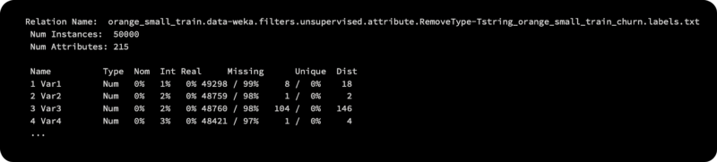
Here is a table that illustrates the dataset:
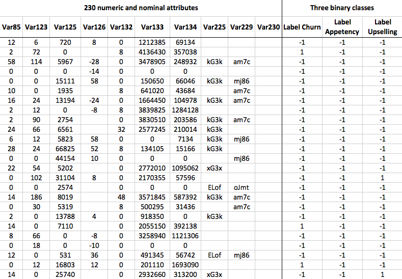
Each customer is described with 250 attributes in the first 25 instances of the table, which are the first 25 examples. Here, we only display a subset of 10 attributes. Several attributes in the dataset have missing values, and some are empty or constant. There are three distinct class labels in the table, namely churn, appetency, and upgrade, which represent the ground truth, or if the customer switched providers (churn). To ensure proper correspondence, it is important to retain the order of the instances and their corresponding class labels separately from the data in three separate files.
Evaluation
Arithmetic mean of the area under the ROC curves was used to evaluate the submissions for the three tasks (churn, appetency, and upselling). As a result of plotting sensitivity versus specificity for various threshold values, the ROC curve shows the performance of the model. AUC is related to the area under the ROC curve — the larger the area, the better the classifier). Weka provides an API for calculating the AUC score, as do most toolboxes.
The baseline for the Naive Bayes classifier
In order to qualify for prizes, participants had to outperform a basic Naive Bayes classifier, which is based on independent features.
There was no feature selection or hyperparameter adjustment for the vanilla Naive Bayes classifier used by the KDD Cup organizers. Naive Bayes’ overall performance on the large dataset was as follows:
Churn problem: AUC = 0.6468
Appetency problem: AUC = 0.6453
Upselling problem: AUC=0.7211
NoThe AUC for upselling is 0.7211.are only reported for the large dataset. On the KDD Cup site, both the training and testing datasets are available, but the test labels are not. We cannot know how well our models will perform on the test set until we process the data with our models. Our models will be evaluated with cross-validation using only training data. We will not be able to compare the results directly, but we will have an idea of what a reasonable AUC score would be.
The data collection process
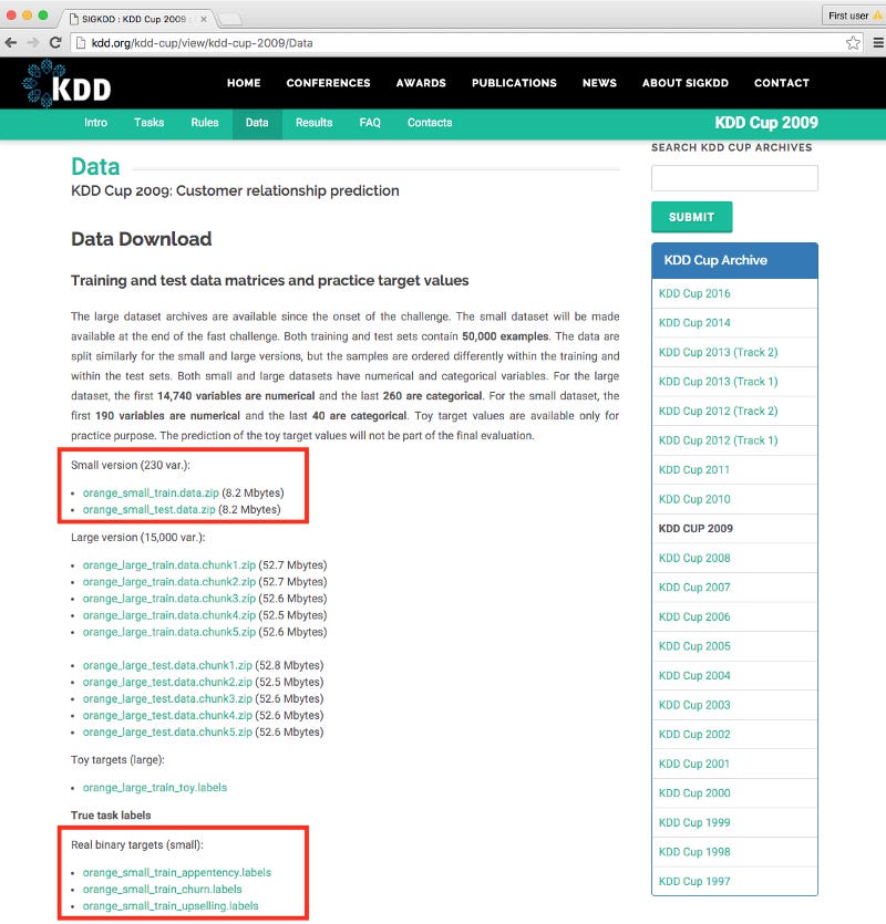
A screenshot of the KDD Cup website can be found at http://kdd.org/kdd-cup/view/kdd-cup-2009/Data. First, download the orange_small_train.data.zip file under the Small version (230 var.) header. After that, you will need to download the three sets of true labels associated with this training data. Below the Real binary targets (small) header are the following files:
orange_small_train_appentency.labels
orange_small_train_churn.labels
orange_small_train_upselling.labels
In the screenshot, all of the files marked in red boxes need to be saved and unzipped:
To determine our baseline AUC scores, we will first load the data into Weka and apply Naive Bayes modeling with the Naive Bayes classifier. A more advanced modeling technique and trick will be discussed later.
Data loading
Our data will be loaded directly into Weka from a .csv file. In order to accomplish this, we will create a function that accepts the path to both the data file and the true labels file. This function loads, merges, and removes empty attributes from both datasets. The first code block will be as follows:

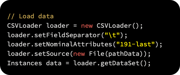
The first step is to load the data using the CSVLoader() class. The last 40 attributes are also forced to be parsed as nominals, using the /t tab as a field separator:
String attributes are automatically recognized by Weka when they don’t contain a single value. Due to the fact that we don’t need them, we can safely remove them with the RemoveType filter. A third parameter, -T, specifies the type of attribute to be removed, as well as the type of attribute to remove:
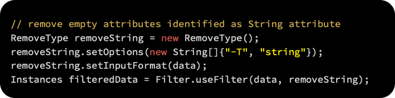
Additionally, we can use the Instances class’s deleteStringAttributes() method, which has the same effect; for example, data.removeStringAttributes().
The data will now be loaded and class labels assigned. Here we’ll use CVSLoader again, specifying that there is no header line in the file, setNoHeaderRowPresent(true):

Once both files have been loaded, a static method Instances.mergeInstances (Instances, Instances) can be called to merge them together. In return, the method returns a new dataset that contains both the first dataset and the second set of attributes. It is important to note that both datasets must have the same number of instances:
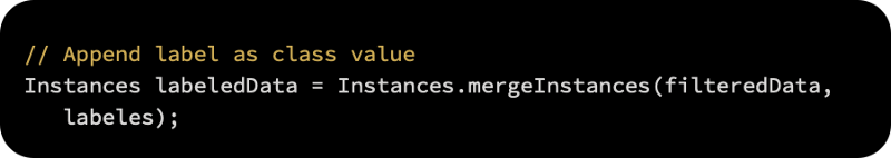
As a final step, we set the label attribute, which we just added, as a target variable, and then return the dataset as follows:

As shown in the following code block, the function provides a summary as output, and returns the labeled dataset:
Modeling basics
Using the approach that the KDD Cup organizers took, we will implement our own baseline model. Let’s first implement the evaluation engine that will return the AUCs for all three problems before we get to the model.
Evaluating models
Let’s examine the evaluation function in more detail. As a result of the evaluation function, the initialized model is cross-validated on all three problems and the results are reported as AUCs:
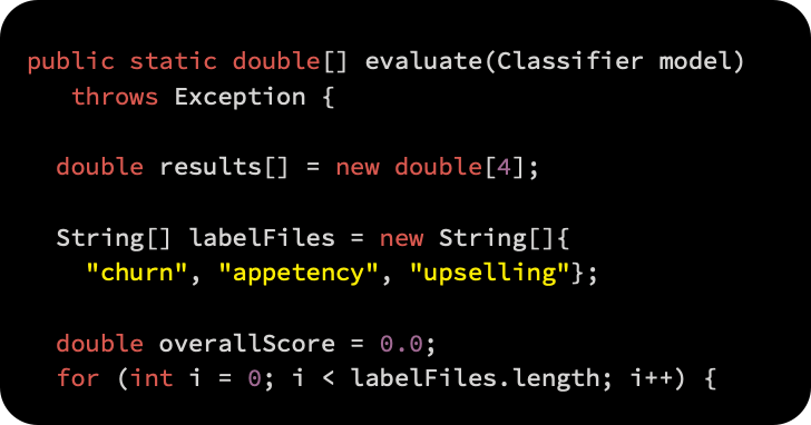
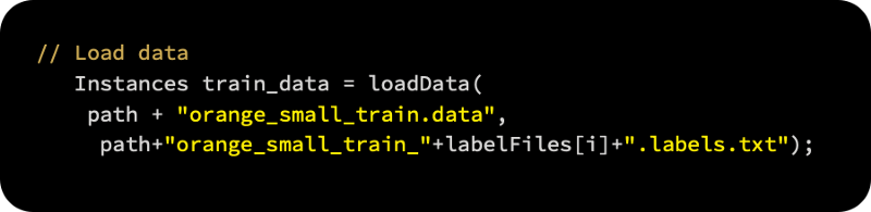
For loading the training data and merging it with the selected labels, we first call the Instance loadData(String, String) function we implemented previously:
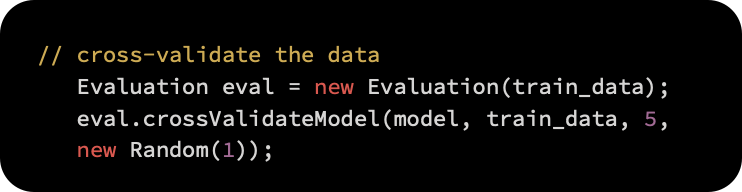
Our dataset is then passed to the weka.classifiers.Evaluation class. (The dataset only serves to extract data properties; the data itself is not considered.) We start cross-validation by calling the void crossValidateModel(Classifier, Instances, int, Random) method. In addition to passing a random seed, we also need a random subset of data for validation:
As soon as the evaluation is complete, we call the double areUnderROC(int) method to read the results. Based on the target value, the method expects an index of the “1” value in the class attribute. This index can be found by searching for the index of the “1” value:
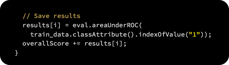
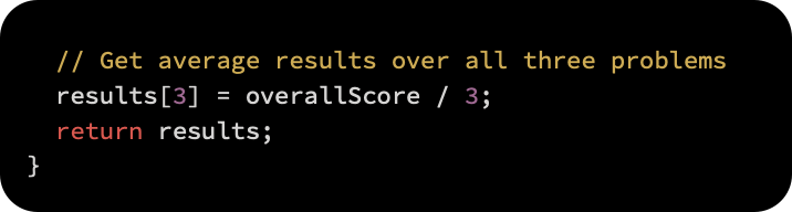
After averaging the results, we return the following:
Naive Bayes baseline implementation
We can now replicate the Naive Bayes approach we expect to outperform once we have all the ingredients. Neither data preprocessing nor attribute selection nor model selection will be included in this approach. We will apply five-fold cross-validation to a small dataset since we do not have true labels for the test data.
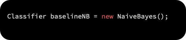
We begin by initializing a Naive Bayes classifier as follows:
Following that, we load the data and apply cross-validation to our evaluation function. ROC curves are produced for all three problems, and the overall results are:
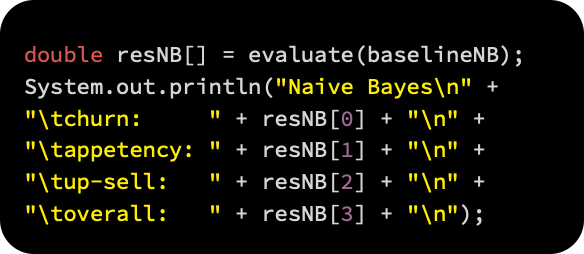
Here are the results of our model:
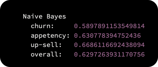
As a baseline, we will use these results when developing more advanced models. By using more complex, time-consuming, and sophisticated techniques to process the data, we expect to achieve much better results. It would be a waste of resources otherwise. A simple baseline classifier is always a good idea when solving machine learning problems.
Ensemble modeling for advanced modeling
Next, let’s look at heavy machinery. We implemented an orientation baseline in the previous section. Our approach will be based on the IBM research team’s KDD Cup 2009 winning solution (Niculescu-Mizil).
The ensemble selection algorithm was used to address this challenge (Caruana and Niculescu-Mizil, 2004). In order to provide the final classification, this is an ensemble method, which combines the output of multiple models in a specific way. In addition to its desirable properties, it is well-suited to this challenge in the following ways:
Performance was excellent, demonstrating its robustness.
AUC is one performance metric that can be optimized.
There is an option to add different classifiers to the library.
A solution is available at any time, so we are never out of options.
Following their report’s steps, we will follow them loosely here. In this article, we are not implementing their approach exactly, but rather providing an overview of the solution, including the steps needed to dive deeper.
These are the general steps:
Preprocessing means removing attributes that don’t add any value to the data — for example, all of the missing or constant values; fixing missing values, so that machine learning algorithms can deal with them; and converting categorical attributes to numerical ones.
Using the attribute selection algorithm, we will select only those attributes that can be helpful in task prediction.
Our third step involves implementing ensemble selection algorithms with a variety of models and evaluating their performance.
Before we begin
EnsembleLibrary is an additional Weka package we will need for this task. Versions 3.7.2 and higher of Weka support external packages, mostly developed by academics. As shown in the following screenshot, WEKA Packages are available on http://weka.sourceforge.net/packageMetaData:
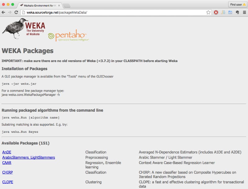
The ensembleLibrary package is available at http://prdownloads.sourceforge.net/weka/ensembleLibrary1.0.5.zip?download.
The ensembleLibrary.jar file should be imported into your code after you unzip the package:
Preprocessing of data
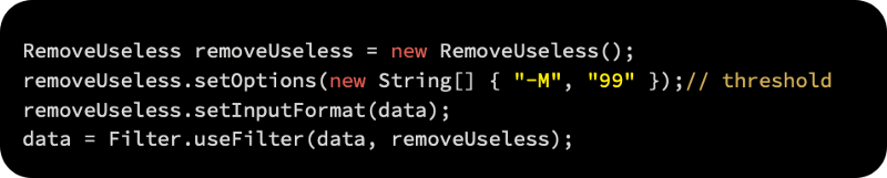
In the first step, we will implement a filter called weka.filters.unsupervised.attribute.RemoveUseless, which does precisely what its name suggests. It removes attributes that aren’t variable much, such as constant attributes. The -M parameter specifies the maximum variance, which applies only to nominal attributes. Attribute values that have unique values in more than 99% of all instances are removed by default, as follows:
Using the weka.filters.unsupervised.attribute.ReplaceMissingValues filter, we will replace all missing values in the dataset with modes (nominal attributes) and means (numeric attributes) from the training data. The replacement of missing values should be approached with caution, taking into account the attributes’ meaning and context:

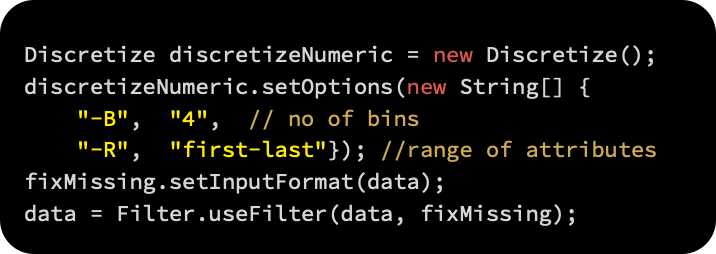
By using the weka.filters.unsupervised.attribute.Discretize filter, we will discretize numeric attributes, converting them into intervals. By using the -B option, numeric attributes are split into four intervals, and by using the -R option, the range of attributes is specified:
Selection of attributes
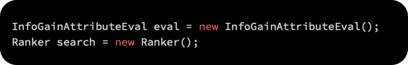
After selecting informative attributes, we will proceed to selecting only attributes that will contribute to prediction. Checking each attribute’s information gain is a standard way of dealing with this problem. We will use the weka.attributeSelection.AttributeSelection filter, which requires two additional components: an evaluator (which calculates attribute usefulness) and search algorithms (which determine which attributes should be considered).
Firstly, we initialize the attribute evaluation implementation weka.attributeSelection.InfoGainAttributeEval as follows:
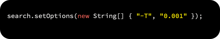
The top attributes with information gain above a threshold are ranked using weka.attributeSelection.Ranker, which initializes the attributes with information gain above a threshold. In order to retain attributes with at least some information, we specify the -T parameter, while keeping the threshold low:
Attribute selection is then applied to the dataset by initializing the AttributeSelection class, setting the evaluator and ranker as follows:
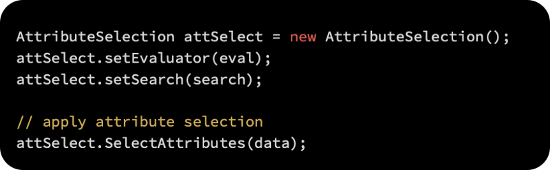
Last but not least, calling reduceDimensionality(Instances) removes the attributes that were not selected in the last run:
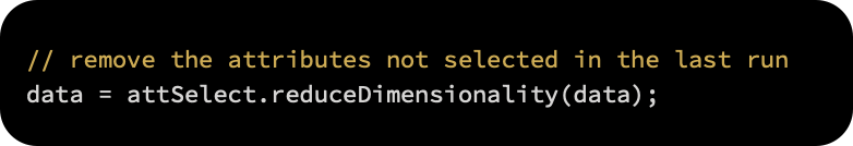
From 230 attributes, 214 remain.
Selection of models
There have been numerous learning algorithms developed by machine learning practitioners over the years and improvements to existing ones have been made as well. Supervised learning methods are so diverse that keeping track of them is challenging. Because datasets vary in characteristics, no one method will work best in every case, but different algorithms can take advantage of the differences and relationships among datasets.
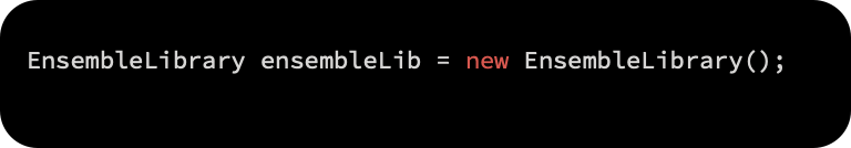
In this step, we will create the model library, which will help us define our models, by initializing the class weka.classifiers.EnsembleLibrary:
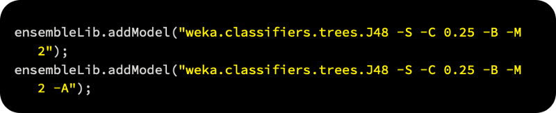
The following is a sample of three decision tree learners, each with different parameters, which we can add as strings to the library:
The following screenshot shows how you can also explore and copy algorithms and their configurations using the Weka graphical interface. Select Edit configuration | Copy configuration string from the right-click menu when you right-click on the algorithm name:

The following algorithms and parameters have been added to this example:
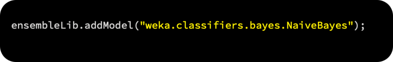
For the default baseline, we used Naive Bayes:
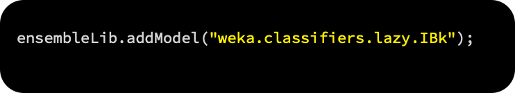
Using lazy models, here are the k-nearest neighbors:
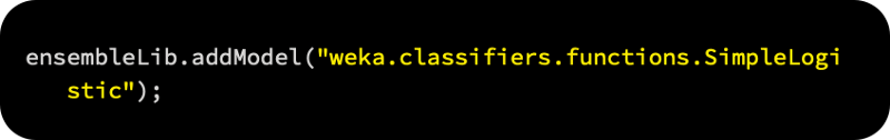
Default parameters for logistic regression:
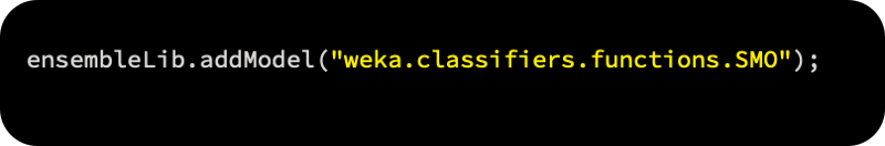
Default parameters for support vector machines:
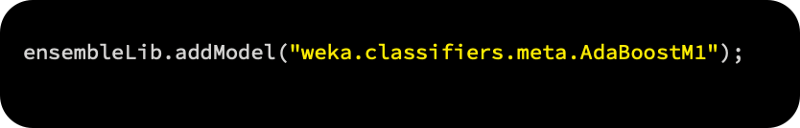
In addition to AdaBoost, which is itself an ensemble method, there are also the following methods:
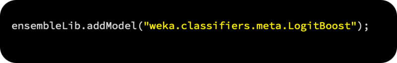
A logistic regression-based ensemble method called LogitBoost:
A one-level decision tree-based ensemble method called DecisionStump:

In EnsembleLibrary, models are saved into files by calling the saveLibrary(File, EnsembleLibrary, JComponent) method, as shown below: