Decoding Market Noise: Building a Neural Network for Algorithmic Trading from Scratch

Download source code using the url at the end of this article!

In the high-stakes world of algorithmic trading, the difference between a profitable strategy and a failed backtest often lies in a model’s ability to distinguish genuine market signal from stochastic noise. While off-the-shelf libraries like TensorFlow or PyTorch offer convenience, they often obscure the mathematical mechanics crucial for understanding model convergence and overfitting — two fatal flaws in financial modeling. This article deconstructs a Feedforward Neural Network (FFNN) down to its raw NumPy foundations. By building the architecture, backpropagation, and momentum optimizers from scratch, we gain the granular control necessary to diagnose how models learn from non-linear market data and, ultimately, how to engineer more robust predictive engines for the stock market.

Training a feedforward neural network using backpropagation

Imports and Settings

import warnings
warnings.filterwarnings(’ignore’)

This pair of lines turns off Python’s warning system for the remainder of the interpreter session by installing a global “ignore” filter. At runtime, warnings emitted by the standard library or by any imported third‑party package (deprecation notices, numerical stability notices, convergence hints, chained‑assignment alerts from pandas, CUDA/cuDNN informational messages surfaced through wrappers, etc.) will be suppressed and not printed to stdout or stderr. Because the call is executed at import time, it affects everything that runs afterwards in this process, including deep learning libraries and data‑processing steps used by our financial prediction pipeline.

Why a developer might do this: in interactive demos or long batch runs we sometimes suppress warnings to reduce noise in logs, make plot outputs cleaner, or avoid overwhelming users with repeated warnings that are already acknowledged. However, in the context of deep neural networks for financial prediction this blanket suppression is risky. Warnings often surface early symptoms of real problems that affect model correctness, stability, or reproducibility — examples include convergence warnings from optimizers, overflow/underflow or NaN propagation in tensors, deprecated API behavior that will change semantics in future library releases, and data handling issues (e.g., pandas’ chained assignment) that can silently mutate inputs and bias predictions. Silencing all warnings makes debugging much harder and can allow subtle errors to persist into production or audit reports.

A safer approach is to be intentional about which warnings you silence. Instead of a global ignore, prefer scoping suppression narrowly (per block or per module) and filtering by specific categories or message patterns so that only known benign warnings are hidden. Capture and log unexpected warnings during training runs and, in CI, treat warnings as errors so regressions are caught early. For libraries that emit noisy but important info (TensorFlow, CUDA), consider library-specific verbosity settings or redirecting those messages to structured logs rather than globally suppressing them. Finally, remember this call mutates global interpreter state — so if someone later expects warnings to be visible for diagnostics, they won’t be unless the filter is explicitly reset — make suppression explicit and documented in the codebase so model maintainers and auditors understand the tradeoffs.

%matplotlib inline

from pathlib import Path
from copy import deepcopy

import numpy as np
import pandas as pd

import sklearn
from sklearn.datasets import make_circles

import matplotlib.pyplot as plt
from matplotlib.colors import ListedColormap
from mpl_toolkits.mplot3d import Axes3D  # 3D plots
import seaborn as sns

This tiny block sets up the computational and visualization environment you’ll use to explore how different neural architectures behave on financial prediction tasks, and it reflects choices that support both experimentation and clear, reproducible visuals.

First, the notebook magic (%matplotlib inline) simply configures the interactive environment so plots are rendered inline in the notebook. That’s important during iterative model development because we want immediate visual feedback — training curves, feature correlations, decision boundaries or embedding projections — without extra steps to open images.

Pathlib.Path and copy.deepcopy are small but purposeful utilities. Path is used for robust, cross-platform file and directory handling when loading raw market data, saving preprocessed datasets, model checkpoints, and experiment artifacts. deepcopy is used when you need independent snapshots of objects — common when implementing early stopping, keeping the best-performing weights during training, or trying variants of preprocessing/pipelines without mutating the original.

NumPy and pandas form the data backbone: NumPy provides performant numerical arrays and operations that feed into tensor construction and custom numeric transforms, while pandas gives the table- and time-series-first functionality you need for financial data (resampling, rolling aggregates, alignment, handling timestamps and missing values). In practice you’ll use pandas to implement feature engineering (sliding windows, returns, volatility, lagged features) and NumPy to efficiently compute these features and to convert them into the array shapes expected by your training code or frameworks.

sklearn is included not merely for its classifiers but for utilities that support experimentation. make_circles is a toy dataset generator for creating a simple, non-linearly separable classification problem; we use it as a diagnostic tool to verify that a neural architecture can represent non-linear decision boundaries. More broadly, sklearn supplies preprocessing (scalers, encoders), model selection (cross-validation, grid search), and metrics that are essential when comparing architectures, tuning hyperparameters, and validating model generalization on financial targets.

The plotting stack (matplotlib, ListedColormap, Axes3D, seaborn) is chosen to cover the range of visual needs in architecture development. Matplotlib gives precise control for custom plots: training loss/accuracy curves, ROC/PR curves, and annotated figures for reports. ListedColormap lets you define consistent color mappings for class visualization (for example, buy/hold/sell labels or default/no-default categories). Axes3D enables 3D scatter or surface plots which are useful when you want to inspect low-dimensional embeddings or the geometry of learned representations from hidden layers — this can reveal separability or pathological collapse that metrics alone would miss. Seaborn sits on top of matplotlib to make statistical visualizations and exploratory plots (pairplots, heatmaps of correlation matrices, distribution plots) that quickly surface feature relationships, skew, and multi-collinearity — insights that directly influence architecture and regularization choices (e.g., whether to add embedding layers, batch normalization, or stronger dropout).

Taken together, these imports are about workflow: reliably loading and snapshotting data and model artifacts, engineering and transforming financial features, creating controlled toy problems to validate model expressiveness, and producing the diagnostic visualizations needed to iterate on neural architectures. The “why” is practical — visual and statistical tools let you detect issues like insufficient model capacity, overfitting, poor feature scaling, or misleading class imbalance early, so you can choose appropriate architectural changes (additional layers, activation choices, normalization, or attention mechanisms) before committing to costly training runs on full market datasets.

# plotting style
sns.set_style(’white’)
# for reproducibility
np.random.seed(seed=42)

These two lines set up two aspects of the experiment that are orthogonal to the core model code but important for running, diagnosing, and communicating results in a production or research context.

The call to set the plotting style to “white” is about presentation and consistency: it standardizes the aesthetic of all subsequent Seaborn/Matplotlib figures so that diagnostic plots — loss curves, learning-rate schedules, validation-vs-train performance, feature distributions, and backtest visualizations — look the same across notebooks, scripts, and collaborators. That consistency reduces visual noise when you compare runs, makes charts easier to read in reports, and helps ensure important signal (e.g., small differences in curves) isn’t obscured by inconsistent gridlines, background color, or default styling. It does not affect model computation, but it does affect how you interpret plots during model development and how you present results to stakeholders and auditors.

Seeding the NumPy random number generator with a fixed value (here 42) is about reproducibility and debuggability. Many parts of a machine-learning pipeline for financial prediction rely on randomness: shuffling and splitting time-adjacent data (or generating bootstrap samples), stochastic weight initialization, synthetic data augmentation, Monte Carlo simulations, and deterministic pseudorandom sampling used in diagnostic scripts. By setting the seed you make the NumPy-based sources of randomness deterministic across runs on the same environment, which helps you reproduce a specific training behavior, isolate bugs, and produce repeatable backtests and figures for review. In a financial context, reproducibility supports auditability and regulatory traceability: you can regenerate a reported result exactly to investigate an anomaly.

Two practical caveats follow from the “why”: first, NumPy’s RNG seed only controls NumPy’s random functions; modern deep-learning frameworks (PyTorch, TensorFlow, cuDNN, CUDA) have their own RNGs and non-deterministic kernels, so for full reproducibility you must also seed those libraries and enable deterministic modes where available. Second, while fixed seeds aid debugging, relying on a single seed can mask sensitivity to initialization or data sampling; for robust model evaluation in finance you should still run experiments across multiple seeds to estimate variance and tail behavior. Finally, always record the seed(s) and the environment (library versions, hardware) in experiment metadata so results remain interpretable and reproducible later.

results_path = Path(’results’)
if not results_path.exists():
    results_path.mkdir()

This code ensures that a filesystem location named “results” exists before the program tries to write any experiment outputs into it. The logic is simple: construct a Path object for “results”, check whether that path already exists, and if it does not, create a directory there. The immediate purpose is to prevent downstream I/O operations (saving model checkpoints, serialized weights, experiment metrics, plots, or CSVs) from failing with a “no such file or directory” error when those artifacts are written during training or evaluation.

In the context of deep neural network architectures for financial prediction, creating this directory up front is important for reproducibility, auditability and operational robustness. Financial experiments typically produce many artifacts (checkpoints for different epochs or hyperparameter settings, evaluation logs, backtests, and feature-importance outputs) that you want persisted reliably for later analysis, model governance, and regulatory review. Ensuring the output directory exists avoids noisy failures that could interrupt long-running training jobs and helps keep experiment outputs organized.

A couple of practical robustness notes and alternatives: using Pathlib is a clean, cross-platform way to express filesystem paths, but the exists-check-then-create pattern as written is not atomic — if multiple processes run this code concurrently you can still hit a race condition where both see the directory missing and one fails when trying to create it. To make this robust, prefer results_path.mkdir(parents=True, exist_ok=True) (or catch FileExistsError) so directory creation succeeds even if another process creates it in the meantime. Also be explicit about where this directory is created by wiring it through configuration (absolute path or a known project root) or by resolving it (results_path.resolve()), and consider using timestamped or run-id subdirectories under “results” to avoid overwriting outputs from different experiments. These changes help ensure reliable, auditable storage of model artifacts and metrics for financial prediction workflows.

Input data

Specification of the expected input.

Generate Random Data

The target variable y denotes two classes generated by circular distributions. These classes are not linearly separable because class 0 surrounds class 1.

We will generate 50,000 random samples arranged as two concentric circles with different radii using scikit-learn’s make_circles function, creating a dataset whose classes are not linearly separable.

# dataset params
N = 50000
factor = 0.1
noise = 0.1

These three lines are not mere constants; they define the statistical character of the synthetic dataset you will feed into the network, and therefore shape every downstream modeling decision (architecture size, regularization, training duration, evaluation expectations).

N = 50000 determines the sample size. For deep networks this is a modest but practical corpus: large enough to fit nontrivial models and reveal overfitting/underfitting behavior, yet small enough to iterate quickly. The choice reflects a tradeoff between statistical power and computational cost — 50k observations give the network a chance to learn higher-dimensional feature interactions that matter in finance, while keeping training time, memory usage, and hyperparameter search feasible. If your model has many millions of parameters you should either increase N or add stronger regularization; if N is reduced, expect higher variance in validation metrics and a need for simpler models or stronger priors.

factor = 0.1 encodes the magnitude of the underlying systematic signal (think of it as a factor loading or the amplitude of a latent driver such as a macro signal or sector exposure). Setting this relatively small makes the true signal subtle compared to raw feature variance, which simulates realistic financial problems where predictable components (alpha) are weak. The practical consequence is that the model must be sensitive to small, consistent patterns rather than relying on large, obvious separations — this favors architectures and training regimes that can extract weak structure (careful normalization, stable optimizers, sufficient depth to capture nonlinearity) and it amplifies the importance of validation procedures because small changes in regularization or data leakage can meaningfully change apparent performance.

noise = 0.1 controls the observation/idiosyncratic noise level added to each sample. Together with factor it defines the signal-to-noise ratio (SNR) of the synthetic market you are modeling. In a Gaussian-additive formulation, equal numeric values for factor and noise imply the signal and noise variances are comparable, producing a challenging but learnable problem. Increasing noise makes the Bayes-optimal error higher and slows convergence; decreasing it makes the task easier but less realistic. Noise also determines which robustness techniques you should prioritize: high noise motivates stronger regularization (weight decay, dropout), robust loss functions, data augmentation strategies, and extensive cross-validation to avoid mistaking noise-fitting for genuine signal.

How these three interact matters more than their absolute values. With N fixed, lowering factor or raising noise reduces effective sample complexity — your network needs more capacity to tease out weaker signals, but more capacity also increases overfitting risk. Practically, treat these parameters as knobs for experimental design: use a grid over factor and noise to probe model sensitivity, evaluate simpler baselines (linear and shallow models) to estimate baseline SNR and achievable performance, and match model capacity to N (parameter count << effective sample size) or compensate with regularization and ensembling. Also consider making the noise more realistic (heteroskedastic or heavy-tailed) if you need stress tests for architectures intended for live financial data.

In short: N sets how much data the network can learn from, factor sets how strong the underlying predictable signal is, and noise sets how obscured that signal is by randomness. Together they define the problem difficulty; tune them thoughtfully based on compute budget, model size, and how faithfully you want to mimic real financial prediction challenges.

n_iterations = 50000
learning_rate = 0.0001
momentum_factor = .5

These three scalar hyperparameters are the control knobs for the core training loop; thinking of them as the choreography of gradient descent helps explain both their immediate mechanics and their role in a financial-prediction pipeline. n_iterations determines how many parameter update steps the optimizer will attempt. In practice this sets the time budget for learning: with noisy, low-signal financial data we often need many steps to let the network discover small, stable patterns, but more steps also increase the chance of overfitting to recent market idiosyncrasies. That’s why you’ll almost always pair a large n_iterations with validation checks, early stopping, and model checkpointing rather than treating it as an unconditional run-to-completion.

learning_rate (1e-4 here) is the scalar that converts gradient direction into a parameter change; it directly controls step size and thus stability vs speed of convergence. For financial prediction the gradients are typically noisy (heteroskedastic returns, regime shifts, sparse signals), so a conservative learning rate helps avoid overshooting and extreme parameter oscillation that would amplify sensitivity to outliers. A small lr makes training slower but more stable — especially important for deep architectures where large steps can destabilize lower layers or blow up activations. Because it slows progress, small learning rates are often used together with longer training schedules or adaptive schemes (decay schedules, warm restarts, or switching to/adopting adaptive optimizers) and you should monitor validation metrics to decide whether lr should be increased, decreased, or scheduled.

momentum_factor implements inertia in the update rule (classical momentum: v = mu * v — lr * grad; params += v). Its purpose is twofold: (1) it damps high-frequency noise in stochastic gradients by averaging directions over time, which is valuable for financial data where single-batch gradients can be misleading, and (2) it accelerates movement through shallow curvature and helps escape small local minima or saddle regions. A value of 0.5 is a moderate amount of inertia — enough to smooth updates but lower than the common 0.9 used in image tasks. That lower setting can be intentional for finance: too much momentum risks carrying the model through regime changes or committing to noisy trends; too little momentum can make convergence slow and oscillatory. The effective behavior depends on the batch size and gradient variance, so momentum and lr must be tuned together.

Operationally, these three parameters interact strongly. With small lr you need more iterations (or an adaptive optimizer) to converge; with higher momentum you can often increase lr slightly because momentum reduces sensitivity to per-step noise, but that can also reduce adaptivity to sudden distributional shifts — an important consideration in financial systems. Because financial targets are non-stationary, treat n_iterations as an upper bound and rely on validation-based stopping, and instrument training with per-iteration logging (train/validation loss, AUC, calibration, and out-of-time tests). Finally, treat these values as starting points: grid or Bayesian tuning, lr schedules (cosine/step/plateau), gradient clipping, weight decay, and trying adaptive optimizers (e.g., Adam with tuned betas) are common next steps to improve stability and generalization in production financial models.

# generate data
X, y = make_circles(
    n_samples=N,
    shuffle=True,
    factor=factor,
    noise=noise)

This line creates a small, controlled toy dataset of two classes arranged as concentric rings and assigns it to X (feature vectors) and y (binary labels). Concretely, X will be an N×2 array of floating-point coordinates and y will be an N-length vector of 0/1 labels; the inner ring has radius equal to factor and the outer ring has radius 1. The factor parameter therefore controls how close the two classes are in feature space (a factor close to 1 makes the rings similar in size and closer to one another; a small factor makes the inner ring much smaller and easier to separate), while the noise parameter injects Gaussian perturbation into the point positions, producing overlap and label uncertainty. shuffle randomizes the order of samples so that subsequent batch-based training does not pick up on any artificial ordering.

Why use this here: make_circles gives you a deliberately nonlinearly separable, low-dimensional problem with tunable difficulty. That makes it ideal for probing the inductive capacity of different deep neural network architectures without confounding issues from real market data (missing values, many correlated features, nonstationarity). By varying factor and noise you can force the model to learn curved decision boundaries (testing activations and depth), expose sensitivity to label noise (testing regularization, dropout, weight decay), and inspect overfitting behavior as you change model size versus sample count N. Because the classes are balanced by construction, performance changes are easier to attribute to architecture and training choices rather than class imbalance.

Practical implications for our financial-prediction workflow: treat this dataset as a diagnostic rather than a benchmark. Preprocess X the same way you would real features (scaling, train/validation split, one-hot or label formatting for the loss), and remember y is binary integers so use an appropriate output+loss (sigmoid+binary-crossentropy or 2-unit softmax). When noise is high and factor yields substantial overlap, prefer stronger regularization or simpler models to avoid overfitting; when the rings are well separated, shallow nets might suffice. Finally, interpret results conservatively — success on make_circles indicates a model can learn complex non-linear boundaries and tolerate controlled noise, but it is not evidence the same architecture will handle the high-dimensional, noisy, and nonstationary structure found in real financial data without further validation and feature engineering.

# define outcome matrix
Y = np.zeros((N, 2))
for c in [0, 1]:
    Y[y == c, c] = 1

This small block constructs a one-hot encoded target matrix Y from a vector of raw class labels y so the network can be trained with a two-output architecture. Conceptually, we want each training example to map to a length-2 vector that marks which of the two outcomes occurred (e.g., “price up” vs “price down”); Y[i] will be [1, 0] when the label y[i] is 0 and [0, 1] when y[i] is 1. The code starts by allocating an N×2 matrix of zeros, then for each class index c ∈ {0,1} it finds all examples whose label equals c and sets the corresponding column c to 1 for those rows. That yields the canonical one-hot format required by many loss implementations.

Why we do this: most classification losses used with small softmax output layers (categorical cross-entropy) expect targets as distributions over classes rather than scalar integer labels. With a two-unit output and softmax you get a probability vector for each example; using one-hot targets lets the loss measure how close that distribution is to the true outcome. In the context of financial prediction, framing up/down or buy/sell as a two-dimensional target lets the model express calibrated probabilities and supports standard evaluation/utility calculations that operate on full probability vectors.

A few practical points about the implementation and assumptions: it assumes y contains integer labels in {0,1} (and that len(y) == N). np.zeros creates a floating matrix, which is appropriate because loss routines expect float targets; the boolean indexing operation Y[y == c, c] = 1 efficiently writes all matching rows at once. The explicit loop over classes is simple and clear for two classes; for more classes you would generalize the loop or use vectorized patterns such as Y[np.arange(N), y] = 1 or np.eye(num_classes)[y] to avoid an explicit Python loop.

Caveats and extensions: if y uses different label encodings (e.g., {−1,1} or strings) you must remap them to 0-based integers before this step. Also choose the target shape to match your network and loss: if you instead use a single sigmoid output and binary cross-entropy, you would keep y as shape (N,) or (N,1) rather than one-hot encode. Finally, for imbalanced financial classes consider augmenting these targets with class weights or focal loss rather than changing the encoding itself.

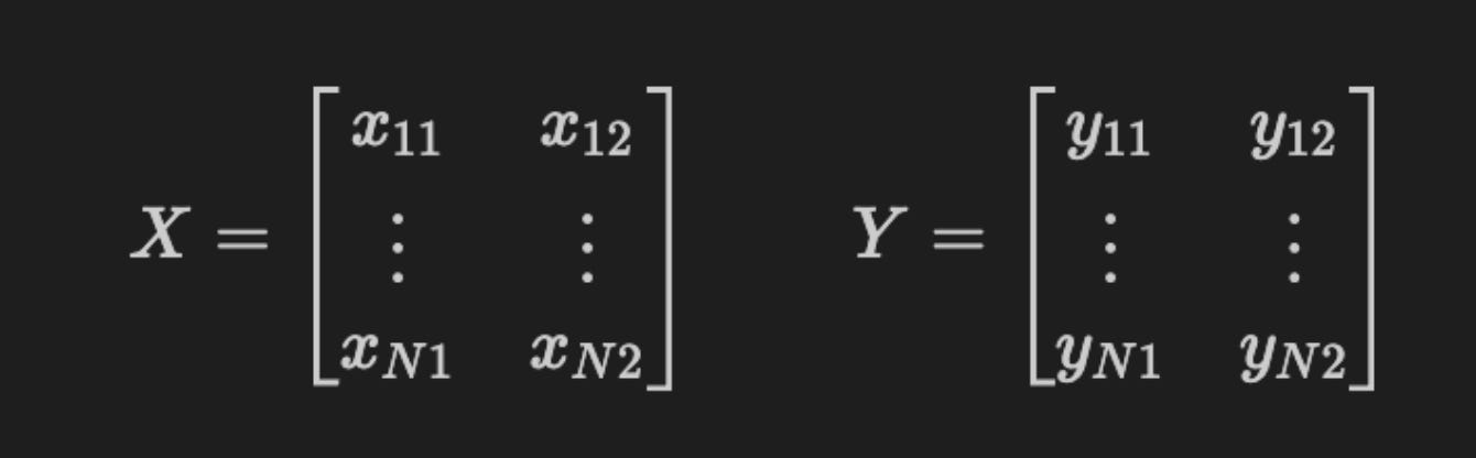
Let X and Y be the following N-by-2 matrices:

f’Shape of: X: {X.shape} | Y: {Y.shape} | y: {y.shape}’

This single f-string is a compact runtime sanity check: it reads the shape tuples of three arrays — X, Y and y — and interpolates them into a human-readable message that you would typically log or print to confirm how the data is structured as it enters the model. Conceptually, X is the feature tensor (for time-series financial inputs this is often shaped as (n_samples, timesteps, n_features) or (n_samples, n_features) depending on the architecture), Y is the label tensor prepared for the loss function (frequently one‑hot encoded for categorical classification, so (n_samples, n_classes)), and y is the raw or scalar form of labels (for example integer class indices or a continuous target used for metrics or inverse-transforming predictions). By emitting these shapes right before training or evaluation you verify the critical invariants the network expects: matching sample counts across inputs and labels, the right rank for sequence models versus fully connected layers, and that label encoding matches the loss/activation choice (sparse vs. categorical).

In the context of deep neural network architectures for financial prediction this check helps catch subtle but high‑impact problems early — e.g., accidentally transposed axes that make timesteps and features swap places, a missing one‑hot conversion so the model receives a 1D label array when a categorical_crossentropy with one‑hot targets is required, or a look‑ahead label misalignment that would introduce leakage. Because shape mismatches typically cause runtime failures or silent training of a misconfigured model, logging X.shape, Y.shape and y.shape is a lightweight, high‑value guard: it documents the pipeline state, aids reproducibility, and directs quick action (assert sample equality, confirm n_classes == Y.shape[1], or reshape/transpose X to match the model input signature) before expensive training runs.

Data Visualization

ax = sns.scatterplot(x=X[:, 0], 
                y=X[:, 1], 
                hue=y,
               style=y,
               markers=[’_’, ‘+’])
ax.set_title(’Synthetic Classification Data’)
sns.despine()
plt.tight_layout()
plt.savefig(results_path / ‘ffnn_data’, dpi=300);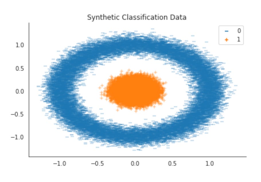

This short block produces a two-dimensional scatter plot of the first two features from X, using the class labels y to encode both color and marker shape, and then saves a publication-quality image. Conceptually the data flows like this: we take X[:, 0] and X[:, 1] as the x and y coordinates so that each row in X is represented as one point in the 2D plane; hue=y assigns a distinct color to each class and style=y assigns a distinct marker to each class (the markers list specifies the glyphs used), so the plot simultaneously communicates class membership by color and by symbol. That dual encoding is intentional: color makes broad cluster structure and class overlap visually obvious, while marker shapes help when color reproduction or color-blind accessibility is a concern or when the plot is printed in grayscale.

Why we do this at this stage is important for model design. Visualizing the first two dimensions gives a quick, interpretable sense of linear separability, cluster shapes, and outliers — key signals for architecture choices in financial prediction tasks. If classes form near-linearly separable regions here, a shallow network or even a linear model might suffice; if they overlap heavily or show complex, nonconvex shapes, that suggests we will need deeper networks, nonlinear activations, or feature transforms (e.g., additional hidden layers, interaction terms, convolutional features if appropriate, or kernel-like expansions). Concentrations of points or extreme outliers indicate whether robust scaling, outlier clipping, or class-specific preprocessing will be necessary, and visible class imbalance warns that loss weighting, sampling strategies, or specialized metrics should be considered during training.

On presentation and reproducibility: sns.despine removes the top/right axes for a cleaner, report-ready look, and plt.tight_layout adjusts margins so labels and titles don’t overlap — useful when generating figures programmatically for papers or dashboards. Finally, plt.savefig writes the resulting figure to results_path / ‘ffnn_data’ at high resolution (dpi=300), which preserves visual fidelity for documentation or model reports; keeping such plots alongside experiment artifacts helps tie visual EDA findings to later architecture and hyperparameter choices during iterative model development.

In short, this block is an EDA visualization step that turns raw feature columns and labels into an immediately actionable visual summary: it informs decisions about model complexity, preprocessing needs, and evaluation strategies before you commit to training deep neural architectures for financial prediction.

Neural network architecture

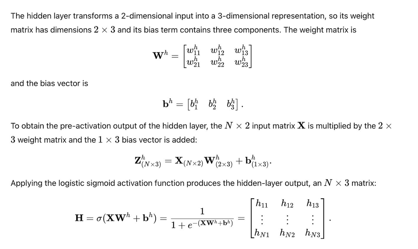
Activations of Hidden Layers

def logistic(z):
    “”“Logistic function.”“”
    return 1 / (1 + np.exp(-z))

This tiny function implements the logistic (sigmoid) activation: it maps any real-valued input z into a value strictly between 0 and 1 via 1 / (1 + exp(-z)). In the context of our deep architectures for financial prediction, that mapping is the key behavior — it turns an unconstrained logit (the linear combination of upstream activations and weights) into a calibrated probability or a gating signal. Practically, you can feed a vector or matrix of logits through this function and get elementwise probabilities that can be interpreted as “probability of positive class,” “probability of a price uptick,” or a continuous risk score that downstream business logic thresholds to make trading or risk-management decisions.

Why we use this shape of nonlinearity is equally important: the logistic function is monotonic and differentiable everywhere, which makes it convenient for gradient-based optimization; when combined with binary cross-entropy loss, the gradient expression simplifies (the derivative of loss w.r.t. pre-activation becomes prediction − label), yielding numerically efficient and stable updates in many cases. Its output range (0,1) also makes it natural for probability calibration, post-hoc metrics (AUC, Brier score), and decision thresholds that map continuous model output to discrete actions or position sizes.

However, the logistic function has well-known practical limitations you need to watch for in financial models. For very large positive or negative logits, exp(-z) underflows/overflows, and the function saturates close to 0 or 1; that saturation causes vanishing gradients in earlier layers and slows or stalls learning if many units operate in that regime. Because of this, we normally prefer ReLU/variants in hidden layers and reserve logistic primarily for final binary outputs or explicit gating units. Also be mindful of numerical stability and precision: use a numerically stable implementation (for example, library expit) or guard against extreme z values, and choose appropriate floating-point precision and weight initialization so logits remain in reasonable magnitudes during training.

Finally, consider the modeling implications in a financial setting: logistic outputs give interpretable probabilities that support risk-aware decisions and calibration checks, but they do not by themselves handle class imbalance or asymmetric costs. You should pair the logistic output with loss weighting, threshold tuning, calibration techniques, or cost-sensitive decision rules to reflect the economic utility of different types of prediction errors (false positives vs false negatives) in trading or risk workflows. For multi-class problems, replace the scalar logistic with softmax; for hidden activations, prefer non-saturating activations to maintain gradient flow.

def hidden_layer(input_data, weights, bias):
    “”“Compute hidden activations”“”
    return logistic(input_data @ weights + bias)

This small function encapsulates a single hidden layer transform: it takes a batch of input feature vectors, linearly projects them into the hidden unit space with a weight matrix and an additive bias, then applies a logistic (sigmoid) nonlinearity to produce the hidden activations that flow to the next layer. Concretely, the matrix product computes each hidden unit’s pre-activation as a weighted sum across the input dimensions, and the bias shifts that pre-activation so units can become active even when the linear combination is near zero; both the weight matrix and bias are the parameters learned by backpropagation to shape these projections for the prediction task.

The choice of the logistic nonlinearity matters for both representational behavior and optimization. Logistic squashes pre-activations into (0, 1), which can be useful when you want hidden units to behave like soft gates or when you need intermediate outputs interpretable as probabilities. However, it also has well-known downsides for deeper architectures: its gradient is proportional to p*(1-p), which becomes very small when units saturate near 0 or 1, so gradients can vanish and slow learning in multi-layer stacks. Because of that, logistic is often appropriate for shallow networks or for specific gating/output units in financial models, but for deeper feature extractors ReLU, leaky ReLU, or other activations are commonly preferred to preserve gradient magnitude and speed convergence.

Operationally there are several practical implications you should keep in mind when this function is used in financial-prediction pipelines. Ensure inputs are appropriately scaled (zero mean/unit variance or similar): without normalization, many pre-activations will sit in the logistic’s saturation zones and learning will be inefficient. Bias should be shaped to broadcast over the batch correctly (typically one bias per hidden unit). Weight initialization matters: small random initial weights avoid initial saturation; if you later move to alternative activations, use initializers matched to them (e.g., He for ReLU). Also consider numerical stability and regularization: logistic can amplify overfitting on non-stationary financial signals, so combine this layer with dropout, weight decay, or batch/layer normalization as needed.

Finally, from an architectural standpoint, wrapping the linear-plus-activation in a single function is useful for modularity and testing, but be deliberate about where you place it in the network. For binary event forecasting or models that explicitly model probabilities, logistic activations make conceptual sense in hidden stages or at the output; for deeper representation learning on noisy, non-stationary financial features you’ll typically prefer activations and structural choices (residual connections, normalization) that mitigate vanishing gradients and improve generalization.

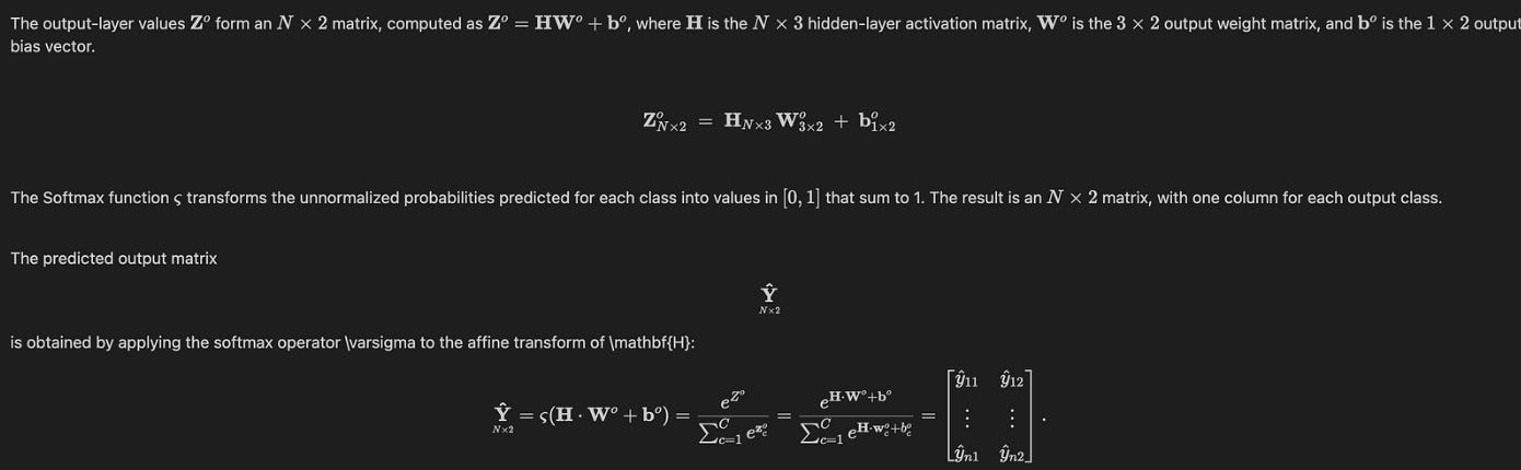
Output activations

def softmax(z):
    “”“Softmax function”“”
    return np.exp(z) / np.sum(np.exp(z), axis=1, keepdims=True)

This function implements the standard softmax mapping used at the output layer of a classifier: it turns each row of raw scores (logits) into a probability distribution over mutually exclusive classes. Conceptually the code first exponentiates each logit (np.exp(z)) to make every transformed score strictly positive and to amplify relative differences between scores; it then divides each exponentiated score by the sum of exponentials for that row so that the values across each row sum to one. In practice we expect z to be shaped (batch_size, n_classes), so the axis=1 sum computes the normalizing constant per sample and keepdims=True preserves a (batch_size, 1) shape so the division broadcasts cleanly back across the corresponding row.

Why we do these two steps (exponentiate then normalize) is important for both interpretation and optimization. Exponentiation ensures monotonicity (higher logits become higher probabilities) and produces a simplex-valued output suitable for cross-entropy loss and probabilistic decision rules (e.g., selecting the class with maximum probability or scoring risk levels). From an optimization perspective, softmax combined with cross-entropy gives a convenient gradient structure — the derivative simplifies in a way that is efficient to compute and stable in well-implemented frameworks — which is why softmax + cross-entropy is the canonical final layer for multiclass classification.

One important practical caveat: the naive implementation shown is vulnerable to numerical overflow when logits have large magnitude, because exp(large) can overflow floating-point ranges. The standard mitigation is to subtract the row-wise maximum from z before exponentiating (exp(z — max_z)), which does not change the normalized probabilities but prevents overflow. Also, when computing loss during training it is more robust to use a fused log-softmax + cross-entropy routine (or a log-sum-exp trick) provided by your ML framework rather than computing softmax and then taking a log separately — that avoids catastrophic cancellation and improves numerical stability.

In the context of deep neural networks for financial prediction, the softmax output is typically the last step when you want calibrated class probabilities (for example, regime classification, discrete actions like buy/hold/sell, or multi-class credit/risk buckets). Keep in mind softmax can produce overconfident predictions when logits are large or the model is overfit; common remedies include temperature scaling or explicit calibration methods. Also consider whether a probabilistic scalar (e.g., predicted return distribution parameters) or ordinal/regression output would better match your financial objective — softmax is appropriate when the problem is truly categorical and you need a probability distribution over discrete outcomes.

def output_layer(hidden_activations, weights, bias):
    “”“Compute the output y_hat”“”
    return softmax(hidden_activations @ weights + bias)

This small function is the final mapping from the network’s hidden representation to a probability distribution over output classes. Sequentially, a batch of hidden activations (typically shaped [batch_size, hidden_dim]) is projected into the output space by a linear map: the activations are multiplied by a weights matrix (hidden_dim × num_classes) and then a bias vector (num_classes) is added. That linear output are the logits — unnormalized scores for each class — and the softmax converts those logits into a normalized probability distribution per example so the model’s output can be interpreted as class probabilities.

We do the matrix multiply because we want a full linear combination of hidden features for each output dimension; the bias term shifts each class’s baseline logit independently, allowing the model to express prior preferences that are not captured by the features alone. Broadcasting semantics are relied on for the bias add (one bias per output class applied to every row of the batch). The softmax step is used because our downstream objective is probabilistic (e.g., categorical cross-entropy) and we need outputs that sum to one and are positive so they can be treated as calibrated probabilities for decision-making in finance (expected-value calculations, risk thresholds, or ranked actions).

Operationally and numerically, treat the logits carefully: you often combine softmax with cross-entropy into a single stable loss implementation (log-sum-exp trick) to avoid overflow/underflow and to get better gradient behavior. During inference, if you only need the top class, you can skip computing the full softmax and take argmax on the logits for efficiency; if you need calibrated probabilities (for risk scoring or portfolio allocation), keep the softmax but consider temperature scaling or calibration techniques. Finally, remember that gradients flow back through both the softmax and the linear projection into the hidden layers and weights, so any regularization (weight decay, dropout applied earlier) or normalization decisions will directly affect the learning dynamics of these final parameters in the context of financial prediction.

Forward propagation

The `forward_prop` function combines the preceding operations to compute the output activations from input data using the given weights and biases. The `predict` function returns binary class predictions for the input data based on those weights and biases.

def forward_prop(data, hidden_weights, hidden_bias, output_weights, output_bias):
    “”“Neural network as function.”“”
    hidden_activations = hidden_layer(data, hidden_weights, hidden_bias)
    return output_layer(hidden_activations, output_weights, output_bias)

This function is the high-level forward pass for a two-stage neural model: it converts raw input features into a prediction by first transforming them into a learned internal representation and then mapping that representation to the output space. Concretely, the incoming batch of input vectors is handed to hidden_layer, which is expected to perform an affine transform with hidden_weights and hidden_bias followed by a nonlinearity (ReLU/tanh/etc.) and any per-layer processing you choose (batch-norm, dropout, etc.). The result, hidden_activations, is an intermediate feature embedding that encodes the nonlinear combinations of the original financial features that the model has learned to be useful for the downstream task.

Those hidden activations are then passed to output_layer along with output_weights and output_bias; output_layer performs the final affine mapping (and possibly a task-appropriate activation such as identity for regression, softmax for multiclass classification, or sigmoid for binary outcomes) to produce the model’s predictions. Separating the computation into hidden_layer and output_layer keeps concerns isolated: the hidden stage is where representation learning and nonlinear feature extraction occur, while the output stage is where those features are projected into the label space and any task-specific scaling or normalization is applied.

From a training and maintenance perspective this structure is beneficial because it is a pure, side-effect-free composition of operations: gradients backpropagate cleanly from the output through the hidden activations to the input, and you can swap or extend the hidden_layer implementation (multiple hidden layers, residual connections, recurrent or attention modules for temporal signals) without changing the outer forward_prop interface. For financial prediction specifically, this design lets you tune the hidden nonlinearity and regularization independently of the final output mapping — critical when you decide whether you’re modeling continuous returns (use linear outputs and MSE, careful about normalization and outliers) or classification outcomes (use softmax/sigmoid with cross-entropy, guard against class imbalance). Finally, because weights and biases are injected as arguments rather than being implicit globals, the function is easy to test, to checkpoint parameter sets, and to use with different optimization schemes or parameter initializations that reduce exploding/vanishing gradients on noisy financial data.

def predict(data, hidden_weights, hidden_bias, output_weights, output_bias):
    “”“Predicts class 0 or 1”“”
    y_pred_proba = forward_prop(data,
                                hidden_weights,
                                hidden_bias,
                                output_weights,
                                output_bias)
    return np.around(y_pred_proba)

This function is the final decision step in a very small prediction pipeline: the input feature matrix (data) is fed through forward_prop together with the network parameters (hidden_weights, hidden_bias, output_weights, output_bias), and whatever scalar values forward_prop emits are then converted into binary class labels by numpy’s rounding operation. In other words, forward_prop is expected to implement the network’s forward pass (hidden-layer transforms, nonlinearities, and a final output activation that produces a probability-like score for class 1), and predict simply maps those continuous scores to discrete 0/1 predictions.

The reason for separating these responsibilities is practical: forward_prop encapsulates the learned model mechanics and returns a soft decision (a probability or score), while predict enforces a concrete trading/classification action by thresholding that score. The current implementation uses np.around, which effectively applies a 0.5 threshold (values below 0.5 become 0, values above 0.5 become 1), so it makes a deterministic decision suitable for downstream rules that require a binary signal (e.g., buy vs. do nothing, approve vs. decline).

There are two important behavioral and business-logic implications to be aware of. First, rounding discards uncertainty: in financial prediction we frequently need calibrated probabilities for risk-adjusted decisions (position sizing, expected value calculation, or cost-sensitive actions). If you need that, return the raw probabilities from forward_prop or expose both probability and hard label. Second, np.around uses “round to even” behavior for exact 0.5 values and can be subtly different from a strict >= 0.5 boolean threshold; for reproducible decision rules it’s safer to use an explicit comparison (y_pred_proba >= threshold) so you can also tune the threshold based on ROC/PR analysis, class imbalance, or economic utility rather than assuming 0.5.

Finally, because this code sits in a financial context where false positives and false negatives have different costs, I recommend two immediate enhancements: (1) tune and expose the decision threshold based on business metrics (expected return, drawdown, cost of errors), and (2) preserve and log predicted probabilities alongside the boolean decision so downstream systems can perform risk-weighted actions or aggregate signals across models.

Cross-entropy loss

The cost function J uses the cross-entropy loss ξ, which sums the discrepancies between the predicted values \hat{y}_{ic} (for each class c and each example i, i = 1,…,N) and the true outcomes.

The loss function is defined as

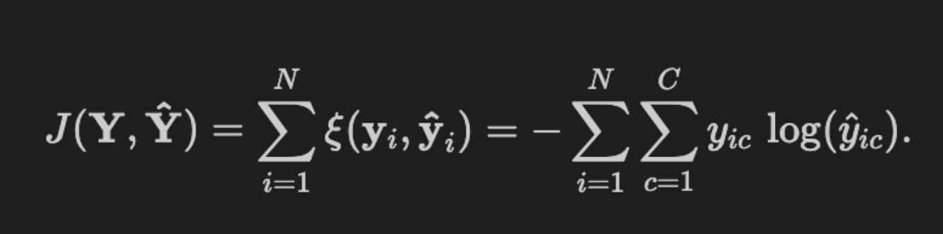
def loss(y_hat, y_true):
    “”“Cross-entropy”“”
    return - (y_true * np.log(y_hat)).sum()

This function implements the scalar cross-entropy loss between predicted probabilities (y_hat) and target distributions (y_true). Conceptually it computes the negative log-likelihood of the targets under the model’s predicted distribution: we take the elementwise product y_true * log(y_hat), sum over the output dimensions, and negate the result. When y_true is a one‑hot vector (typical for single-label classification) this collapses to −log(p_true), i.e. the negative log probability the model assigns to the correct class; when y_true is a full distribution it computes the expected negative log probability under the target distribution. Cross‑entropy is thus a direct maximum likelihood objective and is the natural choice when the model is producing probability estimates (softmax for multi‑class, sigmoid for independent binary outputs).

Why this objective matters for financial prediction: it encourages calibrated probabilities rather than just correct labels, and it penalizes confident mistakes heavily — a desirable property when downstream decisions depend on probability values (risk-adjusted decisions, portfolio weighting, thresholding). Using cross‑entropy aligns training with probabilistic forecasting goals and, through maximum likelihood, gives an interpretable loss surface tied to information‑theoretic divergence (the loss equals the model’s expected negative log probability, and minimized cross‑entropy corresponds to minimizing KL divergence between true and predicted distributions).

There are important practical considerations and common refinements you should be aware of. First, numerical stability: taking log(y_hat) is unsafe if y_hat contains zeros or values extremely close to zero; in practice you must clip y_hat into (eps, 1−eps) or, better, use a fused “softmax + cross-entropy” implementation that computes the loss directly from logits to avoid catastrophic underflow/overflow. Second, the reduction semantics matter: this implementation sums all terms, which yields a scale that grows with number of classes and batch size. For stable learning rate behavior across batch sizes you will normally average (mean) over the batch and often over classes where appropriate. Third, class imbalance and risk preferences in finance often require weighting the loss per class or per sample (e.g., cost‑sensitive weighting) or applying label smoothing to improve calibration and generalization.

Finally, consider how this loss interacts with gradients: when cross‑entropy is paired with softmax, the gradient with respect to the logits simplifies to (y_hat − y_true), which is efficient and numerically well‑behaved when computed in the fused implementation. Also remember to combine this data loss with regularization (L2 on weights, dropout, etc.) and to verify that y_true is a proper distribution (one‑hot or probability vector) and y_hat truly are probabilities (softmax/sigmoid outputs). These choices — numerical stability, reduction, weighting, and regularization — determine whether this simple formula becomes a robust training objective for financial prediction models.

Backpropagation

Backpropagation updates model parameters using the partial derivative of the loss with respect to each parameter, computed via the chain rule.

Gradient of the Loss Function

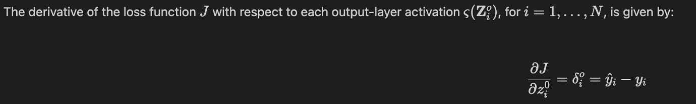
def loss_gradient(y_hat, y_true):
    “”“output layer gradient”“”
    return y_hat - y_true

This tiny function is the entry point for computing the error signal at the network’s output layer: given the model’s predicted probabilities y_hat and the ground-truth targets y_true it returns y_hat — y_true. The intended use is that y_hat is the activation produced by the output unit (typically a softmax for multi-class or a sigmoid for binary tasks) and y_true is a one-hot or probabilistic target. After the forward pass produces y_hat, this function produces the per-output “delta” that will be propagated backward to compute weight gradients in the layers below.

Why the subtraction? Because when you pair a softmax output with the categorical cross-entropy loss (or a sigmoid output with binary cross-entropy), the analytic derivative of the loss with respect to the pre-activation input simplifies to predicted_probability − target. That algebraic cancellation is deliberate: it avoids forming the full softmax Jacobian and yields a compact, numerically efficient error term that directly encodes both the direction and magnitude of the correction needed for each output dimension. In practice that means the returned vector points toward reducing the loss and is the correct starting point for computing weight gradients via the usual backprop chain rule (e.g., multiplying by the previous layer’s activations to get dL/dW).

Operational details you should keep in mind: shapes and batching matter — y_hat and y_true are expected to have identical shapes (batch_size × output_dim), and if your loss implementation averages over the batch you should ensure this gradient is scaled consistently (either the loss or the gradient should include the 1/batch_size). If you use label smoothing, soft targets, or regress real-valued outputs rather than probabilities, the form of the gradient changes and this simple subtraction may no longer be appropriate. Also ensure y_hat is numerically stable (clipped if necessary) when it’s produced, because while the gradient expression avoids explicit logs, the forward-loss computation still needs protection from zeros.

In the context of deep neural network architectures for financial prediction, this compact gradient is a common, efficient choice when the task is probabilistic classification (for example, predicting up/down/flat moves or regime classes). It provides direct, well-scaled signals for learning calibration of probabilities and decision boundaries. That said, financial data often bring class imbalance, non-stationarity and noisy labels, so combine this gradient-driven training with appropriate regularization, class-weighting or resampling, normalization of inputs, and gradient clipping to maintain stable training and robust predictive performance.

Gradients for the output layer

To propagate updates back to the output-layer weights, compute the partial derivative of the loss function with respect to the weight matrix:

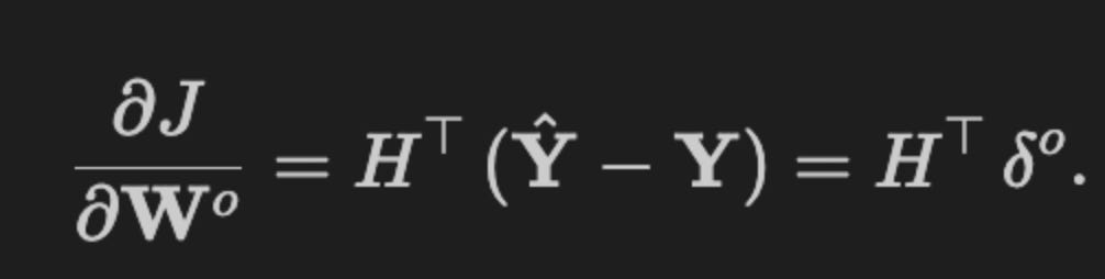
def output_weight_gradient(H, loss_grad):
    “”“Gradients for the output layer weights”“”
    return  H.T @ loss_grad

This small function implements the core mathematical step for computing the gradient of the output-layer weight matrix in a feedforward neural network: given a batch of hidden-layer activations H and the gradient of the loss with respect to the layer’s outputs (loss_grad), it returns the weight gradient by multiplying H^T with loss_grad. The reason this is the correct operation comes from the chain rule applied to a linear output layer y = H W + b: the derivative dL/dW is the sum, across the batch, of each hidden activation vector outer-producted with its corresponding dL/dy vector — and in matrix form that sum is exactly H.T @ loss_grad. This implementation therefore aggregates per-sample contributions efficiently and yields a matrix whose shape matches the weight matrix (hidden_dim × output_dim).

Shape and data-flow considerations are important: H is expected to be (batch_size, hidden_dim) and loss_grad (batch_size, output_dim), so the matrix product sums over the batch dimension to produce (hidden_dim, output_dim). Because the operation sums contributions across samples, you must decide whether to scale or average by batch_size later (many training loops divide this result by batch_size so updates reflect mean gradients rather than raw sums). Also ensure loss_grad represents the gradient with respect to the linear outputs (i.e., after any chain-rule propagation through activation functions) so this multiplication computes the correct parameter gradient.

From a performance and numerical standpoint, the vectorized matrix multiply is preferred: BLAS-backed matrix multiplication is far faster and more memory-efficient than explicit loops over samples. In financial prediction, where labels are noisy and gradients can be high-variance, you should combine this gradient calculation with standard defenses — e.g., minibatch averaging, gradient clipping, appropriate learning-rate schedules or adaptive optimizers, and L2 weight decay — to prevent unstable updates. If you use regularization like weight decay, apply it explicitly to this gradient before updating weights.

Finally, conceptually this step is where learned feature exposures (the columns of W) are adjusted according to how each hidden feature correlates with the loss signal. That mapping is central to tailoring network representations to financial targets, so correctness (shapes and ordering), scaling (batch averaging), and stabilization (regularization/optimizer choices) around this simple H.T @ loss_grad operation have outsized impact on model robustness and predictive performance in production financial systems.

Update: Output Bias

To update the output-layer bias values, we likewise apply the chain rule to compute the partial derivative of the loss function with respect to the bias vector:

def output_bias_gradient(loss_grad):
    “”“Gradients for the output layer bias”“”
    return np.sum(loss_grad, axis=0, keepdims=True)

This small function computes the gradient of the loss with respect to the output-layer bias by summing the per-example gradients across the batch. In a forward pass the output bias is added equally to every sample’s pre-activation (z = Wx + b), so the derivative of the loss with respect to that scalar/vector bias is the sum over examples of the derivative with respect to each sample’s pre-activation. Practically, loss_grad is expected to be dL/dz for each sample and output unit with shape (batch_size, n_outputs); summing with axis=0 collapses the batch dimension and yields one gradient per output unit.

keepdims=True preserves the resulting array as shape (1, n_outputs) rather than (n_outputs,), which is important for broadcasting and for consistency with downstream code or optimizer state that expects a 2D bias shape. Note also the semantic choice of sum versus mean: summing gives the total gradient across the batch (common when learning-rate schedules or batch-size-aware updates are used), while some codebases prefer to average to make the effective step size independent of batch size — choose the convention that matches your optimizer and training regimen.

In the context of deep networks for financial prediction, this bias gradient adjusts global offsets in the model’s output (for example, systematic under- or over-prediction across many samples). Keeping the update vectorized and shaped correctly (using numpy.sum and keepdims) makes the operation efficient and immediately usable in the subsequent parameter update step (e.g., b -= lr * grad).

Gradients for Hidden Layers

def hidden_layer_gradient(H, out_weights, loss_grad):
    “”“Error at the hidden layer.
    H * (1-H) * (E . Wo^T)”“”
    return H * (1 - H) * (loss_grad @ out_weights.T)

This small function computes the backpropagated error signal for a hidden layer given the error at the network output and the weights connecting hidden units to outputs. Conceptually it implements the chain rule step that answers the question: “how much did each hidden unit contribute to the current loss?” Concretely, loss_grad is the gradient coming out of the output layer for each sample in the batch; multiplying it by the transpose of the output weight matrix projects that output error back onto each hidden unit, producing an upstream error per hidden neuron. That projected error is then multiplied elementwise by H * (1 — H), which is the derivative of the sigmoid activation (assuming H contains the hidden-layer activations). The result is the delta for each hidden activation (dL/dH) that you would use to compute gradients for the hidden-layer weights or to continue propagation further back.

On shapes and data flow: loss_grad is expected to be (batch_size, output_dim) and out_weights arranged so that out_weights.T has shape (output_dim, hidden_dim); thus loss_grad @ out_weights.T yields (batch_size, hidden_dim) — one error value per hidden unit per sample. H must have the same (batch_size, hidden_dim) shape and be the post-activation outputs (not the pre-activation linear terms), so the elementwise product H * (1 — H) correctly applies the activation derivative. This preserves batch-wise parallelism and avoids explicit loops.

Why this matters for financial prediction models: we need accurate, stable credit assignment from outputs back into hidden representations because small errors in the forecast can depend on subtle feature interactions encoded in hidden units. Using the sigmoid derivative here enforces that the error is scaled by the local sensitivity of each hidden unit; saturated hidden units (H near 0 or 1) will therefore receive very small updates, which both explains and warns about the vanishing-gradient behavior that can hamper deep networks. In practice for deep or highly noisy financial tasks you may prefer activations and architectural choices (ReLU/LeakyReLU, batch normalization, residual connections, gradient clipping, L2 regularization) to mitigate vanishing/exploding gradients and stabilize training.

Finally, be mindful of numerical and implementation details when integrating this function: ensure H truly is the post-activation sigmoid output, confirm consistent weight-shape conventions, avoid in-place operations that mutate H if you need it later, and consider scaling or clipping gradients when training on volatile financial time series to keep learning stable.

Hidden weight gradient

def hidden_weight_gradient(X, hidden_layer_grad):
    “”“Gradient for the weight parameters at the hidden layer”“”
    return X.T @ hidden_layer_grad

This function implements the standard backpropagation step that computes the gradient of the loss with respect to the hidden-layer weight matrix by accumulating contributions from a batch of examples. Conceptually, each sample i in the batch contributes an outer product between its input vector x_i and the derivative of the loss with respect to the hidden pre-activation z_i (often written ∂L/∂z_i). By forming X.T @ hidden_layer_grad you perform those outer products for the whole batch in a single, efficient matrix multiply: X has shape (batch_size, input_dim), hidden_layer_grad is (batch_size, hidden_dim), so the result has shape (input_dim, hidden_dim), matching the hidden weight matrix W. This implementation therefore returns the aggregated gradient ∑_i x_i (∂L/∂z_i)^T.

Why we do it this way: backpropagation separates the gradient wrt pre-activation (∂L/∂z) from the activation derivative and from the upstream layers so the weight update is simply the input times that pre-activation gradient. Using a batched matrix multiplication is both mathematically correct and computationally optimal (leveraging BLAS/GPU kernels) compared to looping over samples. Note that hidden_layer_grad must already include the derivative through the activation function (i.e., it should be ∂L/∂a * ∂a/∂z) and that bias gradients are handled separately unless you’ve augmented X with a constant column.

Practical considerations for financial prediction systems: this routine returns the summed gradient across the minibatch, not the mean — so remember to divide by batch_size if your learning-rate schedule or optimizer expects averaged gradients. Also consider adding L2 regularization (weight decay) to the returned gradient, and apply gradient clipping or normalization when working with volatile financial inputs to prevent exploding updates. Finally, ensure X is the same preprocessed input used in the forward pass (normalization/scaling saved or recomputed) because gradient magnitudes and stability depend heavily on input scaling in financial time-series models.

Hidden-Bias Gradient

def hidden_bias_gradient(hidden_layer_grad):
    “”“Gradient for the bias parameters at the output layer”“”
    return np.sum(hidden_layer_grad, axis=0, keepdims=True)

This small function takes the per-sample gradient that arrives from the layer’s activation (commonly dL/dz where z = W x + b) and reduces it into the gradient for the bias parameter of that layer. Concretely, hidden_layer_grad is expected to be a 2‑D array shaped (batch_size, n_units) containing the contribution to the loss for each example and each output neuron; because the bias b is shared across all examples, the correct parameter gradient is the sum of those per-sample contributions. The function therefore sums along axis 0 (the batch axis), producing a 1×n_units row vector whose entry j is ∑_i dL/dz_{i,j}.

The keepdims=True option preserves the 2‑D shape (1, n_units), which keeps the gradient shape consistent with how biases are typically stored (e.g., a row vector) and avoids broadcasting/shape-mismatch issues during later, vectorized update steps. Note this routine returns the summed batch gradient rather than an average; many training loops will divide by batch_size or adjust the learning rate elsewhere if they want an average gradient. From a modelling perspective, collapsing per-sample signals into a single bias update stabilizes learning across a mini‑batch and ensures the bias shifts the activation thresholds based on the aggregate directional signal — important in financial prediction models where systematic offsets across many examples must be corrected. The implementation is fully vectorized (no Python loops), relying on NumPy to efficiently accumulate the gradient across the batch.

Initializing Weights

def initialize_weights():
    “”“Initialize hidden and output weights and biases”“”

    # Initialize hidden layer parameters
    hidden_weights = np.random.randn(2, 3)
    hidden_bias = np.random.randn(1, 3)

    # Initialize output layer parameters
    output_weights = np.random.randn(3, 2)
    output_bias = np.random.randn(1, 2)
    return hidden_weights, hidden_bias, output_weights, output_bias

This small function’s job is to create the initial trainable parameters for a two-layer neural network used in our financial prediction pipeline: one hidden layer with three units and an output layer with two units. The shapes encode the flow of data — hidden_weights is (input_dim=2, hidden_units=3), hidden_bias is (1, 3), output_weights is (hidden_units=3, output_dim=2), and output_bias is (1, 2). In practice this means when a batch of inputs X with shape (batch_size, 2) is fed forward, X @ hidden_weights produces a (batch_size, 3) pre-activation for the hidden layer; adding hidden_bias (broadcast across the batch) and applying an activation gives the hidden activations, which are then multiplied by output_weights and shifted by output_bias to produce the final (batch_size, 2) network outputs.

The function uses samples from a standard normal distribution to break symmetry between units: random initialization prevents every neuron from learning the same features and gives stochastic starting directions to the optimizer. However, a plain standard-normal draw is a naive choice and has important implications for optimization. If weights are too large, activations can saturate (for sigmoids/tanh) or produce exploding activations/gradients; if too small, signals can vanish. Those issues are particularly relevant in financial prediction where inputs are often normalized but can exhibit heavy tails and nonstationarity; poor initialization will slow convergence or lead to suboptimal local minima when training on noisy market data.

Because of those risks, a production-ready approach should parameterize the layer sizes rather than hard-coding (2 and 3 and 2), and use principled initializers matched to the activation function and layer fan-in/fan-out — e.g., Xavier/Glorot for tanh/sigmoid, He initialization for ReLU/LeakyReLU — to control the variance of activations through the network. Also consider deterministic seeding for reproducibility, and initialize biases to zero (a common pattern) unless there’s a reason to inject a small offset. Finally, tie this back to the business goal: for financial prediction we must pair robust initialization with careful input preprocessing (scaling, outlier handling), appropriate output activations and loss (classification vs regression), and regularization (dropout, weight decay) to improve generalization on volatile, nonstationary market data.

Computing Gradients

def compute_gradients(X, y_true, w_h, b_h, w_o, b_o):
    “”“Evaluate gradients for parameter updates”“”

    # Compute hidden and output layer activations
    hidden_activations = hidden_layer(X, w_h, b_h)
    y_hat = output_layer(hidden_activations, w_o, b_o)

    # Compute the output layer gradients
    loss_grad = loss_gradient(y_hat, y_true)
    out_weight_grad = output_weight_gradient(hidden_activations, loss_grad)
    out_bias_grad = output_bias_gradient(loss_grad)

    # Compute the hidden layer gradients
    hidden_layer_grad = hidden_layer_gradient(hidden_activations, w_o, loss_grad)
    hidden_weight_grad = hidden_weight_gradient(X, hidden_layer_grad)
    hidden_bias_grad = hidden_bias_gradient(hidden_layer_grad)

    return [hidden_weight_grad, hidden_bias_grad, out_weight_grad, out_bias_grad]

This function implements the backward pass for a two-layer network by following the chain rule in a readable, modular way: it first performs the forward pass needed for backprop, then computes gradients for the output layer, and finally propagates those gradients into the hidden layer and its parameters. The overarching goal here — training a deep architecture for financial prediction — is to provide correct, testable gradients for updating the hidden weights/biases and output weights/biases so the model can reduce prediction error on financial targets (prices, returns, or class probabilities).

We start by computing and caching the hidden-layer activations and the network output (y_hat). Caching hidden_activations is important because the weight gradients for the output layer depend on those signals, and the hidden-layer gradients require them too; avoiding redundant recomputation keeps training efficient when working with large financial datasets. The code then computes loss_grad: an abstraction that yields dL/dy_hat according to the chosen loss (so you can swap MSE for regression or cross-entropy for classification without changing the rest of the backprop code). This abstraction matters for finance because you might change the objective depending on whether you’re forecasting a continuous return or classifying an event.

Next, the function computes the output-layer parameter gradients. out_weight_grad is derived by correlating the incoming signals from the hidden layer with the loss gradient at the outputs (conceptually hidden_activations^T · loss_grad), because the derivative of the loss with respect to an output weight equals the activation of the upstream neuron times the downstream gradient. out_bias_grad is simply the aggregate downstream gradient across the batch (since bias gradients do not multiply an input). Computing these first is natural: output parameters are closest to the loss and their gradients are needed both for updates and for propagating error backward.

After the output gradients are known, the code computes the hidden-layer gradient by backpropagating the output gradient through the output weights and the hidden activation nonlinearity. The hidden_layer_gradient function encapsulates that chain-rule step (effectively multiplying loss_grad by w_o^T and then elementwise by the derivative of the hidden activation). From that hidden-layer error signal, hidden_weight_grad is computed by correlating input features X with the hidden-layer error (conceptually X^T · hidden_layer_grad), and hidden_bias_grad is the batch-wise sum of the hidden error. These quantities are exactly what you need to perform SGD/Adam-style parameter updates for the hidden layer.

Finally, the function returns the gradients in a predictable ordering [hidden_weight_grad, hidden_bias_grad, out_weight_grad, out_bias_grad]. That order should match the optimizer or update routine that consumes these gradients. Practical considerations for financial models: because financial targets are noisy and nonstationary, you’ll typically pair this gradient calculation with regularization (weight decay, dropout), gradient clipping, and careful choice of loss to avoid exploding or misleading updates; those concerns are intentionally handled outside this function so the backprop math remains clean and reusable.

Gradient Checking

# change individual parameters by +/- eps
eps = 1e-4

# initialize weights and biases
params = initialize_weights()

# Get all parameter gradients
grad_params = compute_gradients(X, Y, *params)

# Check each parameter matrix
for i, param in enumerate(params):
    # Check each matrix entry
    rows, cols = param.shape
    for row in range(rows):
        for col in range(cols):
            # change current entry by +/- eps
            params_low = deepcopy(params)
            params_low[i][row, col] -= eps

            params_high = deepcopy(params)
            params_high[i][row, col] += eps

            # Compute the numerical gradient
            loss_high = loss(forward_prop(X, *params_high), Y)
            loss_low = loss(forward_prop(X, *params_low), Y)
            numerical_gradient = (loss_high - loss_low) / (2 * eps)

            backprop_gradient = grad_params[i][row, col]
            
            # Raise error if numerical and backprop gradient differ
            assert np.allclose(numerical_gradient, backprop_gradient), ValueError(
                    f’Numerical gradient of {numerical_gradient:.6f} not close to ‘
                    f’backprop gradient of {backprop_gradient:.6f}!’)

print(’No gradient errors found’)

This block is a classic gradient-checking routine: its goal is to validate that the gradients returned by your backpropagation implementation (compute_gradients) match numerical gradients computed from the loss function. Correct gradients are critical for training deep networks used in financial prediction because tiny errors in gradient computation can lead to poor convergence or systematic bias in model updates, which in turn can materially affect downstream forecasts and risk decisions.

Flow and decisions: first you initialize the model parameters and compute the analytic gradients once via compute_gradients(X, Y, *params). Those gradients are the “ground truth” from your backpropagation code that you want to verify. Then the code iterates each parameter matrix and each scalar element inside those matrices. For the current element it constructs two perturbed parameter sets (params_low and params_high) that differ from the original only at that single element by -eps and +eps respectively; deepcopy ensures the rest of the parameter arrays remain unchanged so the perturbation is isolated. The forward_prop is then run for both perturbed parameter sets to get model outputs, and the loss is computed on each output (loss_high and loss_low). Using the central difference formula (loss_high − loss_low) / (2 * eps) yields a numerical approximation of the partial derivative with respect to that scalar parameter. This central-difference estimate is chosen because it is symmetric and generally more accurate (O(eps²)) than a one-sided difference.

After computing the numerical gradient, the code compares it to the corresponding entry in grad_params (the backprop gradient) using np.allclose and asserts they are sufficiently close; if they are not, an error is raised and the developer is alerted to a discrepancy. This comparison implicitly assumes that the ordering and shapes returned by initialize_weights and compute_gradients align exactly, and that the loss used for numerical checking includes whatever terms (e.g., regularization) the analytic gradient accounts for — mismatches there are a frequent source of false positives.

Why these choices matter here: eps must be small enough to approximate the derivative yet large enough to avoid floating-point round-off errors; 1e-4 is a common compromise but may need tuning depending on loss scaling in financial datasets. Deep copying each parameter set isolates the perturbation so you are truly checking a single partial derivative. Using the central difference reduces bias in the numerical estimate. And elementwise checking gives fine-grained assurance that every scalar gradient is implemented correctly, which is important in financial models where unexpected weight interactions can produce subtle but consequential errors.

Practical notes and caveats: this method is computationally expensive (nested loops and two forward passes per parameter element), so it’s appropriate as a debugging tool on small models or on a random subset of parameters rather than during normal training. Also ensure consistency between the analytic gradient computation and the loss used for numerical checking (include regularization, dropout handling should be deterministic or disabled during checking, etc.). Finally, consider comparing with a tolerance tuned for your problem (np.allclose’s atol/rtol) and, for larger networks, using vectorized perturbations or flattened-parameter checks to reduce runtime.

Train network

def update_momentum(X, y_true, param_list,
                    Ms, momentum_term,
                    learning_rate):
    “”“Update the momentum matrices.”“”
    # param_list = [hidden_weight, hidden_bias, out_weight, out_bias]
    # gradients = [hidden_weight_grad, hidden_bias_grad,
    #               out_weight_grad, out_bias_grad]
    gradients = compute_gradients(X, y_true, *param_list)
    return [momentum_term * momentum - learning_rate * grads
            for momentum, grads in zip(Ms, gradients)]

This function implements the velocity update step of a classical momentum-based optimizer: given the current minibatch (X, y_true) and the current parameter values, it computes gradients and produces new momentum (velocity) vectors that will be applied to the parameters elsewhere. First, compute_gradients is called with the input batch and the four parameters (hidden layer weights and bias, output layer weights and bias). That call encapsulates the backpropagation logic and returns a list of gradient arrays ordered to match param_list; keeping the ordering consistent is crucial because the momentum matrices Ms are expected to correspond to the same parameter ordering.

Next, the function combines each previous momentum with its corresponding gradient in a single vectorized expression. For each pair (momentum, grads) it computes momentum_term * momentum — learning_rate * grads. Multiplying the old momentum by momentum_term preserves and decays the historical velocity (the “why”: this carries forward a smoothed direction built from past gradients, which helps accelerate convergence along persistent descent directions and damp oscillations), while subtracting learning_rate * grads moves the velocity in the negative gradient direction (the “how”: scaling by learning_rate controls step magnitude). The negative sign enforces gradient descent rather than ascent. Using zip and a list comprehension keeps the update order and shapes aligned so each parameter gets its matching updated velocity.

Importantly, this function only returns updated momentum vectors; it does not mutate the parameters themselves. That separation keeps the optimizer logic modular: parameter updates (e.g., param += new_momentum) happen in the caller, which can also implement additional steps such as bias correction, weight decay, or gradient clipping. In the context of financial prediction, where gradients can be noisy and data non-stationary, the momentum term helps smooth updates across minibatches and reduces sensitivity to sharp, spurious gradient changes — improving stability and often speeding up convergence when training deep architectures on time-series features. Practical considerations you should keep in mind when tuning this block are the choice of momentum_term (commonly 0.9), the learning_rate scale, and whether to add explicit gradient clipping or regularization to handle outliers in financial returns.

def update_params(param_list, Ms):
    “”“Update the parameters.”“”
    # param_list = [Wh, bh, Wo, bo]
    # Ms = [MWh, Mbh, MWo, Mbo]
    return [P + M for P, M in zip(param_list, Ms)]

This small helper applies a precomputed set of parameter updates to the model parameters in one pass. Conceptually it receives two parallel lists: param_list holds the current trainable tensors for the layer block in the order [Wh, bh, Wo, bo], and Ms holds the corresponding updates to apply (MWh, Mbh, MWo, Mbo). The function walks through those pairs (zip) and produces a new list where each parameter has been incremented by its matching update (P + M). Because the function returns a new list rather than mutating in place, it cleanly separates the “compute updates” step from the “apply updates” step.

Why addition? In this design Ms is expected to already encode the optimizer’s sign and scaling (learning rate, momentum, weight decay, etc.). That means any gradient signs, learning-rate multiplications and other optimizer transforms have been applied when forming Ms; update_params’ job is merely to materialize those computed changes onto the parameters. This separation keeps optimizer logic (how to compute M from gradients) decoupled from parameter assignment and makes unit testing and reasoning about updates simpler.

There are some important practical constraints that determine how this code is used in a production training loop for financial prediction. The ordering of param_list and Ms must match exactly — Wh must pair with MWh, and so on — otherwise you will corrupt weights and biases. The shapes and dtypes must be compatible so the elementwise addition is valid; if you are operating on GPU-backed tensors (e.g., PyTorch, TensorFlow), both items in each pair must be on the same device. Also be explicit about sign conventions: if updates were computed as -learning_rate * gradient, addition applies the negative step; if they are raw gradients, the caller must convert them to appropriately signed steps before passing them in.

Because financial models are particularly sensitive to overfitting, nonstationarity and exploding updates, keep additional safeguards around this function: compute and apply gradient clipping, learning-rate schedules, and regularization before forming Ms; consider checks (length equality, shape assertions) during development to catch misalignment bugs; and be mindful whether you want an in-place update (to save memory) or an immutable replacement (safer for debugging and checkpointing). In short, update_params is intentionally minimal: it’s the final “apply these optimizer-produced changes” operation in the training pipeline, and its correctness depends on the upstream optimizer logic that produced Ms.

def train_network(iterations=1000, lr=.01, mf=.1):
    # Initialize weights and biases
    param_list = list(initialize_weights())

    # Momentum Matrices = [MWh, Mbh, MWo, Mbo]
    Ms = [np.zeros_like(M) for M in param_list]

    train_loss = [loss(forward_prop(X, *param_list), Y)]
    for i in range(iterations):
        if i % 1000 == 0: print(f’{i:,d}’, end=’ ‘, flush=True)
        # Update the moments and the parameters
        Ms = update_momentum(X, Y, param_list, Ms, mf, lr)

        param_list = update_params(param_list, Ms)
        train_loss.append(loss(forward_prop(X, *param_list), Y))

    return param_list, train_loss

This function is the high-level training loop that iteratively adjusts the network parameters to minimize prediction error on the provided training set (X → Y). It follows the standard pattern for a momentum-based optimizer but is written so the low-level gradient and parameter-update details are delegated to two helper routines, keeping the training flow compact and easy to read.

At the start we obtain the trainable parameters from initialize_weights() and convert them to a list; param_list holds the weight matrices and bias vectors in a fixed order (the code comment suggests something like [W_h, b_h, W_o, b_o]). Those initial values are important: small random initial weights break symmetry across neurons so the network can learn heterogeneous features from financial inputs, and well-chosen initial scales help avoid saturating activations and vanishing/exploding gradients during early iterations. Immediately after initialization the code builds a matching list of momentum matrices Ms using zeros_like for each parameter; each Ms entry is a velocity/moment accumulator for the corresponding parameter, initialized to zero so the first update is driven purely by the first gradient estimate.

Before entering the loop we compute and record the initial training loss using forward_prop(X, *param_list) and loss(…). Recording the pre-update loss gives a baseline to measure training progress and to detect problems early (e.g., if the initial loss is NaN or extremely large, something is wrong with preprocessing, targets, or initialization).

The loop then runs for the specified number of iterations. Each iteration advances the optimizer one step: update_momentum(…) is called with the current data, parameters, momentum matrices, the momentum factor mf, and the learning rate lr. Its job is to compute gradients (via backprop inside it) and update the moment/velocity terms according to the chosen momentum rule (for example classical exponential moving average of gradients). Using separate momentum matrices makes the optimizer more robust to the noisy, non-stationary gradients typical in financial time-series; momentum smooths updates, speeds travel through shallow directions, and reduces oscillation across steep, narrow valleys in the loss surface. After the updated moments are returned, update_params(param_list, Ms) applies those moments to the actual parameters — this separation keeps the gradient accumulation logic distinct from the parameter application, which makes it easy to swap in other parameter update rules (e.g., Nesterov, Adam) without changing the training loop.

After applying the update the loop recomputes the forward pass and appends the new training loss to train_loss. Collecting the loss history at each step (or at regular intervals) is essential for diagnostics: it lets you plot learning curves, detect divergence or plateauing, and tune lr and mf accordingly — critical when designing deep architectures for financial prediction where overfitting and regime changes are real risks. The loop also prints a progress marker every 1000 iterations (i % 1000 == 0) with immediate flush so you get runtime feedback for long jobs.

Finally, the function returns the learned param_list and the train_loss history. The parameters are used for inference or further evaluation, while the loss trace supports model selection and hyperparameter tuning. In short, this routine orchestrates initialization, momentum-based gradient updates, loss tracking, and progress reporting — providing a compact yet flexible training backbone suited to iteratively refining deep network weights in the noisy environment of financial prediction.

trained_params, train_loss = train_network(iterations=n_iterations, 
                                           lr=learning_rate, 
                                           mf=momentum_factor)

This single-line call hands control to a training routine that turns an untrained architecture into a usable predictive model. Conceptually, train_network is the place where the model’s weights are initialized (or resumed), data batches are pushed through the forward pass to produce predictions, and the discrepancy between predictions and targets is quantified by a loss function appropriate to the financial prediction task (e.g., MSE for regression, cross-entropy for classification). The function runs for n_iterations iterations of whatever update loop the implementation uses (full-batch, mini-batch, or stochastic), so the first decision the call makes is how many weight-update steps the optimizer should perform.

The two hyperparameters you pass in — lr (learning_rate) and mf (momentum_factor) — directly control the optimizer’s behavior. The learning rate determines the step size along the gradient direction: too large and training diverges or oscillates, too small and convergence is prohibitively slow or gets stuck in shallow minima. The momentum factor modifies the plain gradient step by accumulating a fraction of the previous update to damp oscillations and help traverse narrow valleys or saddle points; in noisy financial datasets this helps stabilize updates and accelerate convergence across correlated features. In other words, lr controls how far we move each step and mf smooths the trajectory of those moves.

Inside each iteration the routine typically executes the sequence: (1) compute a forward pass on a batch, (2) compute loss and (optionally) any regularization term, (3) backpropagate to get gradients, and (4) update parameters using an optimizer that uses lr and mf. Along the way the code may keep diagnostics: a running or epoch-level train loss to monitor convergence, optional validation loss computations for early stopping, and occasional checkpointing of trained parameters. That diagnostic stream is why the function returns train_loss alongside trained_params — train_loss is the scalar (or history array) you inspect to confirm that the model is learning and to detect overfitting or non-convergence.

The returned trained_params encapsulate the learned weights (and usually biases and optimizer state if you plan to resume training). You use these parameters for inference on new financial data, for backtesting strategies, or for further fine-tuning. Practically, because financial time-series are non-stationary and noisy, you should treat train_loss as a signal rather than proof: complement it with validation metrics, consider early stopping, learning-rate schedules, gradient clipping, and weight decay to prevent overfitting or exploding gradients. Finally, ensure reproducibility (seed, deterministic dataloaders) and persist checkpointed trained_params so model deployment or analysis uses the exact weights the training produced.

hidden_weights, hidden_bias, output_weights, output_bias = trained_params

This line extracts the four parameter tensors that define a simple two-layer neural predictor: the weight matrix and bias vector for the hidden transformation, and the weight matrix and bias scalar/vector for the output transformation. In the forward pass these play the canonical roles: inputs (normalized financial features) are multiplied by hidden_weights and shifted by hidden_bias, then an elementwise nonlinearity produces the learned latent representation; that latent vector is then multiplied by output_weights and shifted by output_bias to produce the final score or logits that feed into your loss/decision function (e.g., regression value, probability via sigmoid, or class logits followed by softmax). Conceptually, hidden_weights/hidden_bias implement the feature extraction and interaction modeling stage (capturing patterns like momentum, cross-feature interactions, regime-dependent signals), while output_weights/output_bias map those latent features onto the business target (price move, default risk, etc.) and provide the final calibration.

The unpacking also encodes an assumption about ordering and shape conventions that is important in practice: trained_params must be a sequence of exactly four elements and each tensor’s shape and dtype must match the inference code’s expectations (e.g., whether you use row-major weights of shape (in_features, out_features) or the transposed convention affects the matmul). Maintaining this separation is useful for clarity and for applying different treatments — regularization, per-layer learning rates, or post-training calibration — because you can address hidden and output parameters independently. In production, validate the shapes and device placement immediately after unpacking and confirm that the parameter ordering matches how the model packaged the checkpoint; otherwise you risk silent shape-mismatch bugs or miscalibrated predictions that are particularly costly in financial applications.

Plot the training loss

This plot shows the training loss over 50,000 iterations using 50,000 training samples, with a momentum of 0.5 and a learning rate of 1e-4.

The loss does not begin to decline until after roughly 5,000 iterations, but then decreases rapidly. We did not use stochastic gradient descent, which would likely have significantly accelerated convergence.

ax = pd.Series(train_loss).plot(figsize=(12, 3), title=’Loss per Iteration’, xlim=(0, n_iterations), logy=True)
ax.set_xlabel(’Iteration’)
ax.set_ylabel(’$\\log \\xi$’, fontsize=12)
sns.despine()
plt.tight_layout()
plt.savefig(results_path / ‘ffnn_loss’, dpi=300)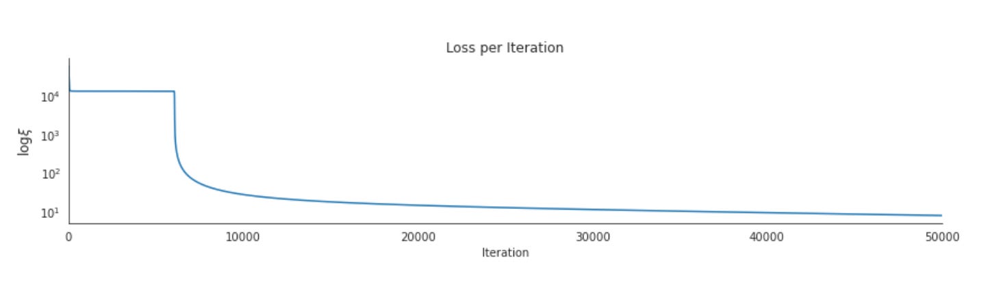

This block produces and saves a compact diagnostic plot of training loss across iterations so you can visually assess optimization behavior during the FFNN training run. The training loss list is wrapped into a pandas Series and plotted with a wide, short figure (12×3) which intentionally emphasizes the temporal progression of loss rather than vertical amplitude; that aspect ratio is useful for spotting trends, plateaus, or recurring spikes over many iterations common in financial-model training. The x-axis is constrained to (0, n_iterations) to keep the horizontal scale consistent across runs and to prevent an accidental mismatch between reported iteration count and plotted points from hiding boundary behavior.

Crucially, the y-axis is plotted on a logarithmic scale (logy=True). We do this because training losses in deep networks frequently span several orders of magnitude early in training or across hyperparameter sweeps; a log scale compresses multiplicative changes so you can see both large early reductions and fine-grained later improvements in the same view. That makes it easier to detect exponential convergence, learning-rate-induced jumps, or failure modes like stagnation or divergence that would be visually obscured on a linear scale. The y-axis label uses LaTeX-style formatting (‘$\\log \\xi$’) to indicate that the plot is showing the logarithm of the loss value xi, clarifying interpretation for downstream reviewers and reproducibility records.

Aesthetic and layout steps are included to produce a publication-quality artifact: seaborn.despine() removes the top and right axes spines for a cleaner look that focuses attention on the data, and plt.tight_layout() adjusts margins to prevent label clipping. Finally, the figure is saved to the results directory as ‘ffnn_loss’ at 300 DPI so the diagnostic can be embedded into reports or dashboards without loss of clarity. In practice, this saved artifact becomes a key part of the training log for financial prediction experiments — used to validate convergence behavior, compare hyperparameter settings, and detect issues (e.g., exploding/vanishing gradients, unsuitable learning rates, or noisy objectives caused by market non-stationarity).

Decision boundary

The following plots show the function learned by a neural network with a three-dimensional hidden layer, trained on two-dimensional data containing two classes that are not linearly separable (left). The decision boundary misclassifies very few points and would likely improve with additional training.

The second plot shows the representation of the input data learned by the hidden layer. The network adjusts the hidden-layer weights so that projecting the inputs from two to three dimensions enables linear separation of the two classes.

The final plot illustrates how the output layer implements this separation using a threshold: outputs above 0.5 are assigned to one class and those below 0.5 to the other.

n_vals = 200
x1 = np.linspace(-1.5, 1.5, num=n_vals)
x2 = np.linspace(-1.5, 1.5, num=n_vals)
xx, yy = np.meshgrid(x1, x2)  # create the grid

# Initialize and fill the feature space
feature_space = np.zeros((n_vals, n_vals))
for i in range(n_vals):
    for j in range(n_vals):
        X_ = np.asarray([xx[i, j], yy[i, j]])
        feature_space[i, j] = np.argmax(predict(X_, *trained_params))

The first part of this block constructs a two-dimensional sampling grid over a fixed range: two linearly spaced arrays define the coordinate axes and meshgrid combines them into pairwise (x1, x2) coordinates. Conceptually, you are enumerating a dense set of input combinations for two features so you can evaluate the trained network on a systematic, regular sweep across that local feature space. In the context of financial prediction, those two axes usually stand for two normalized, high-importance inputs (for example a return measure and a volatility measure, or two principal components). Choosing the interval [-1.5, 1.5] and n_vals = 200 is a design decision that trades off coverage and resolution — it assumes your inputs were scaled into a comparable range during training, and it produces a 200×200 grid fine enough to reveal decision contours while remaining computationally manageable.

Next, the code initializes feature_space as a 2-D array to hold the model’s discrete predictions across the grid. The nested loop iterates through each coordinate pair (xx[i,j], yy[i,j]) and packages it into a vector X_ that is handed to predict along with the trained parameters. predict presumably runs a forward pass of the neural network and returns either class-score logits or class probabilities; applying np.argmax to the output converts that continuous score vector into a single class index (the class with maximum score). Storing that index at feature_space[i,j] builds a map of the network’s class decision at every sampled input location. The loop structure makes the logic explicit: for every candidate input, evaluate the model, pick the most likely class, and record it.

Why do this? The resulting feature_space encodes the model’s decision regions and boundaries in the chosen 2-D projection of the input space. For financial models, visualizing these regions helps validate that the network’s behavior aligns with domain expectations (e.g., smooth boundaries where appropriate, no absurdly fragmented regions that indicate overfitting, or unexpected predictions in economically implausible areas). It is also useful for interpretability and debugging: you can overlay training points to see if the learned boundaries separate classes as intended, inspect confidence near boundaries, and look for regions where tiny input perturbations flip the predicted action (high sensitivity or instability).

A few practical considerations and ways to improve robustness: ensure the grid coordinates are normalized exactly like the training data (mismatched scaling will produce meaningless maps); the choice of two axes is a projection and can miss higher-dimensional interactions, so use PCA or feature importance to pick informative axes; n_vals controls granularity — higher values reveal more detail but increase compute cost quadratically. Performance-wise, the double Python loop is easy to read but slow for large grids; vectorizing by reshaping the grid to a batch and calling predict once (or in batches) will use the network’s optimized matrix operations and drastically reduce runtime. Finally, consider storing full probability vectors (or max-probabilities) instead of just argmax if you need to assess confidence, calibration, or produce continuous decision surfaces (e.g., contour plots of class probabilities) rather than only hard class labels.

# Create a color map to show the classification colors of each grid point
cmap = ListedColormap([sns.xkcd_rgb[”pale red”],
                       sns.xkcd_rgb[”denim blue”]])

# Plot the classification plane with decision boundary and input samples
plt.contourf(xx, yy, feature_space, cmap=cmap, alpha=.25)

# Plot both classes on the x1, x2 plane
data = pd.DataFrame(X, columns=[’$x_1$’, ‘$x_2$’]).assign(Class=pd.Series(y).map({0:’negative’, 1:’positive’}))
sns.scatterplot(x=’$x_1$’, y=’$x_2$’, hue=’Class’, data=data, style=y, markers=[’_’, ‘+’], legend=False)
plt.title(’Decision Boundary’)
sns.despine()
plt.tight_layout()
plt.savefig(results_path / ‘boundary’, dpi=300);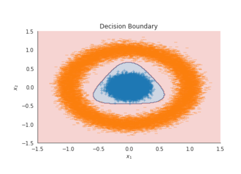

This block is responsible for drawing a two-dimensional visualization of the model’s classification surface and the original data points so you can inspect how the neural network is partitioning the feature space. Upstream, xx and yy are the meshgrid coordinates that cover the range of the two input features and feature_space is the model’s prediction on that grid (typically a 2D array of class labels or probabilities thresholded to labels). The first line builds a small, explicit colormap with two visually distinct colors pulled from seaborn’s xkcd palette; using ListedColormap ensures the contour plotting uses exactly these two colors for the two classes, which keeps the decision regions consistent and readable.

Next, plt.contourf(xx, yy, feature_space, cmap=cmap, alpha=.25) paints the classification plane: each mesh cell is colored according to the predicted class, producing contiguous regions that represent the model’s decision areas. The alpha=.25 makes that background layer translucent so the overplotted sample points remain clearly visible; this balance helps you evaluate where the model’s regions overlap or diverge relative to the actual samples without overpowering the markers.

The code then prepares the observed dataset for plotting. Converting X to a DataFrame and mapping the integer labels y to the strings ‘negative’ and ‘positive’ provides explicit, human-readable class labels which seaborn uses for color/group semantics. sns.scatterplot draws the original samples on top of the decision plane using x1 and x2 as coordinates; passing style=y with markers [‘_’, ‘+’] ensures each numeric class gets a distinct marker shape (underscore vs plus) in addition to color, which is useful when color printing or subtle shading could obscure class separation. legend=False disables the automatic legend here (often done when the figure is part of a multi-panel layout or a separate legend is added elsewhere).

Finally, a few aesthetic and output steps: sns.despine removes the top/right axes spines for a cleaner, publication-style look, and plt.tight_layout prevents label/title clipping so the figure elements don’t overlap. plt.savefig(results_path / ‘boundary’, dpi=300) writes the visualization to disk at a high resolution suitable for reports or slides; saving at 300 dpi ensures crisp lines and readable markers when printed or embedded in documentation. Overall, this visualization provides an immediate, diagnostic view of how the deep model’s nonlinear decision boundary aligns with financial samples in the two-feature projection, helping you spot misclassifications, overly complex boundaries, or regions where more data or regularization might be needed.

Projection onto the Hidden Layer

n_vals = 25
x1 = np.linspace(-1.5, 1.5, num=n_vals)
x2 = np.linspace(-1.5, 1.5, num=n_vals)
xx, yy = np.meshgrid(x1, x2)  # create the grid
X_ = np.array([xx.ravel(), yy.ravel()]).T

This block constructs a 2‑D grid of input points that you can feed to a model or visualization routine to probe how a neural network behaves across a range of feature values. The implicit goal here — given our project on deep neural network architectures for financial prediction — is to create a systematic set of synthetic scenarios (625 points in this case) spanning a controlled range for two features so we can visualize decision surfaces, inspect prediction contours, or run sensitivity/stress tests.

We start by specifying n_vals = 25 to control grid resolution: each axis will have 25 evenly spaced samples, so the full grid contains n_vals**2 = 625 points. Choosing 25 is a tradeoff between resolution and compute cost — finer grids give smoother visualizations but increase inference time quadratically in 2D and exponentially in higher dimensions. The two axes x1 and x2 are produced with linspace over [-1.5, 1.5], which typically represents a standardized range around zero (roughly ±1.5 standard deviations) when working with normalized financial features; selecting this interval lets you inspect model behavior near typical and moderately extreme values but keeps the domain compact.

meshgrid takes those two 1‑D arrays and produces two 2‑D coordinate matrices (xx, yy) that together represent every combination of the x1 and x2 values. This is the key step that turns independent axis samples into a Cartesian grid of (x1, x2) locations. The subsequent ravel() calls flatten those 2‑D matrices into 1‑D vectors and stacking them then transposing yields a shape (625, 2) array (assigned to X_) where each row is one input sample [x1_value, x2_value]. Because meshgrid with default settings repeats x1 across rows and ravel flattens row‑wise, the ordering will vary x1 fastest while x2 increments more slowly — useful to know if you later reshape predictions back to a 2‑D array for plotting.

A couple of practical considerations tied to why this is done: always make sure the grid range and scaling match the preprocessing used during model training (standardization, clipping, PCA, etc.), otherwise the results won’t reflect in‑distribution behavior. Also note the dimensionality curse — grids are fine for 2D contours or pairwise interactions, but become intractable as the number of features grows; for higher dimensions prefer random sampling, sliced projections, or targeted sensitivity analyses. Finally, this grid is intended for batch evaluation (single forward pass per point or batched inference) so you can produce decision boundary plots, compute gradient-based saliency across the domain, or perform scenario stress tests that are easy to interpret in the context of financial prediction.

fig = plt.figure(figsize=(6, 4))
with sns.axes_style(”whitegrid”):
    ax = Axes3D(fig)

ax.plot(*hidden_layer(X[y == 0], hidden_weights, hidden_bias).T,
        ‘_’, label=’negative class’, alpha=0.75)
ax.plot(*hidden_layer(X[y == 1], hidden_weights, hidden_bias).T,
        ‘+’, label=’positive class’, alpha=0.75)

ax.set_xlabel(’$h_1$’, fontsize=12)
ax.set_ylabel(’$h_2$’, fontsize=12)
ax.set_zlabel(’$h_3$’, fontsize=12)
ax.view_init(elev=30, azim=-20)
# plt.legend(loc=’best’)
plt.title(’Projection of X onto the hidden layer H’)
sns.despine()
plt.tight_layout()
plt.savefig(results_path / ‘projection3d’, dpi=300)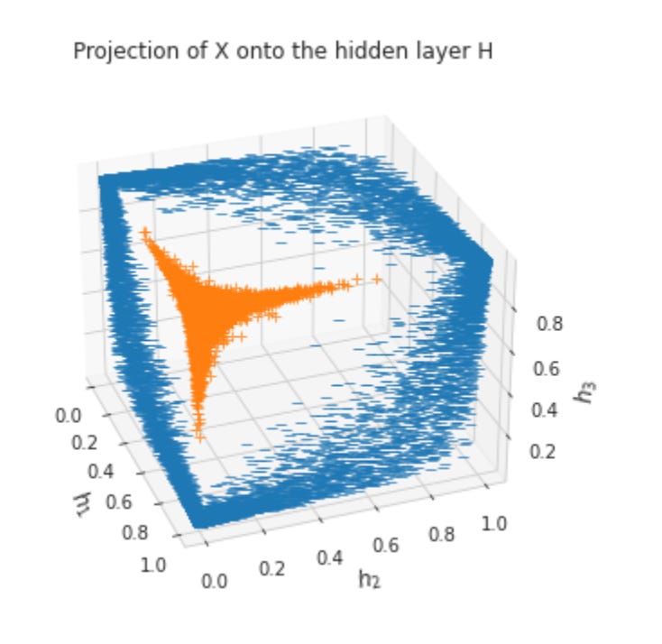

This block produces a diagnostic 3‑D visualization of the network’s hidden representation so you can directly inspect how the model is projecting financial input data into the hidden layer space. Concretely, the code applies the hidden_layer transform (using hidden_weights and hidden_bias) to the rows of X, separately for samples labeled negative (y == 0) and positive (y == 1). The hidden_layer is expected to output a 3‑dimensional vector per sample (h1, h2, h3), and the transpose/unpacking is just a concise way to feed those three coordinates into the 3‑D plotting call. Splitting by label before the projection keeps visualization decisions local to interpretation — we’re not changing the model, just observing how its learned linear+nonlinear mapping organizes the two classes.

The choice of marker styles (‘_’ for negative and ‘+’ for positive) and an alpha less than 1 are deliberate: different markers make class membership immediately visible, and transparency helps reveal point density and overlap where many samples project to similar coordinates (important with financial datasets that often have clusters or heavy tails). Setting the axis labels to h1, h2, h3 ties the plot back to the network’s hidden-unit coordinates rather than raw features, which clarifies that we’re evaluating representation quality rather than feature distributions. The view_init call fixes the elevation and azimuth so the saved image presents a consistent viewpoint across experiments.

Styling and saving are practical but purposeful choices: seaborn’s “whitegrid” gives a neutral background that highlights structure, despine removes distracting spines for a cleaner figure, tight_layout prevents label clipping, and a high DPI plus an explicit figsize produce a publication‑quality artifact you can compare across hyperparameter runs. Note that the legend call is commented out — you may enable it interactively if you need an explicit legend, but it’s often omitted in saved figures to reduce clutter.

Interpretively, this plot is a quick sanity and model‑selection tool for financial prediction: if positive and negative samples form distinct clusters in this 3‑D hidden space, the current hidden layer already learns discriminative features and a simple readout may suffice; if they overlap heavily, it signals that the architecture (number of units, nonlinearity), feature preprocessing, or regularization may need adjustment. Because this is a post‑hoc diagnostic, use it alongside quantitative metrics (loss, ROC/AUC, calibration) to guide architecture and training decisions rather than as the sole criterion.

Network Output: Surface Plot

zz = forward_prop(X_, hidden_weights, hidden_bias, output_weights, output_bias)[:, 1].reshape(25, -1)
zz.shape

This single line is taking the network’s forward pass outputs, selecting a specific output channel, and reorganizing those values into a 2‑D grid so they can be consumed by the next stage of the pipeline. Concretely, forward_prop(…) executes the model on the input batch X_ using the supplied hidden and output weights/biases and returns a 2‑D array of outputs per example (commonly a probability vector or logits per class). The slice [:, 1] picks the second column across all examples — in a binary-up/down financial prediction this is typically the model’s predicted probability (or score) for the “positive” class (e.g., price-up). Choosing the probability rather than argmax preserves the continuous score needed for ranking, calibration, or portfolio weighting rather than just a hard label.

After extracting that score vector, reshape(25, -1) reorganizes the flat 1‑D array of scores into a matrix with 25 rows and however many columns are required to accommodate all examples (the -1 infers the appropriate number of columns). The practical reason for this reshaping is to align predictions with a downstream structure: for example, grouping predictions by 25 assets, 25 time steps, or 25 instruments per mini‑batch so you can compute per‑asset metrics, aggregate returns, or apply vectorized portfolio operations across columns. Note the reshape will fail unless the total number of examples is divisible by 25, so the code implicitly assumes the data ordering and batch size match that grouping.

A couple of important considerations tied to model design: slicing [:,1] assumes forward_prop already produced class probabilities (e.g., via softmax); if it returned raw logits you should be explicit about applying softmax if you need probabilities for calibration or ranking. Also, using the probability channel is intentional for downstream financial tasks — expected return estimation, ranking, or risk-weighted allocation — whereas argmax would lose that nuance. Finally, the zz.shape inspection is a quick sanity check to confirm the grouping (it will print a tuple like (25, N/25)), and it’s good practice to assert the expected divisibility and to document what the 25 represents so future maintainers know why predictions are batched that way.

fig = plt.figure()
with sns.axes_style(”whitegrid”):
    ax = fig.gca(projection=’3d’)
ax.plot_surface(xx, yy, zz, alpha=.25)
ax.set_title(’Learned Function’)
ax.set_xlabel(’$x_1$’, fontsize=12)
ax.set_ylabel(’$x_2$’, fontsize=12)
ax.set_zlabel(’$y$’, fontsize=12)
ax.view_init(elev=45, azim=-20)
sns.despine()
fig.tight_layout()
fig.savefig(results_path / ‘surface’, dpi=300);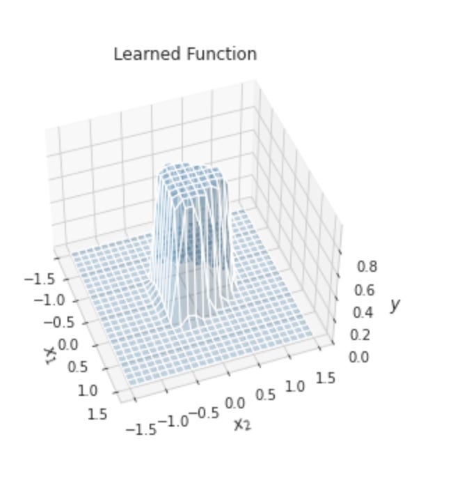

This small block constructs and persists a 3D diagnostic plot of the model’s learned mapping from two inputs to the predicted target; its purpose in the context of deep neural network architectures for financial prediction is to let you visually inspect how the model combines two features (x1, x2) into an output (y), so you can detect nonlinearity, sharp curvature, interaction effects, or pathological extrapolation that would warrant architectural or feature-engineering changes.

Narratively: we create a new figure and enter a seaborn style context to get a clean whitegrid background (improves readability in presentations and reports). A 3D axis is obtained (projection=’3d’) because we are plotting a surface defined by a mesh of input values (xx, yy) with corresponding model outputs zz; these arrays are the meshgrid and the model-predicted z-values over that grid. plot_surface renders the learned function as a continuous surface; alpha=.25 makes it semi-transparent so underlying elements (axes, any overlaid scatter of actual training points you might add elsewhere) remain visible and the shape is easier to interpret visually rather than being a blocking opaque object.

After drawing the surface the code adds a descriptive title and LaTeX-style axis labels for clarity (using explicit font sizes to ensure legibility in saved figures). view_init sets a fixed elevation and azimuth so the same viewpoint is used across runs — this consistency is important when you compare surfaces between different model variants or training checkpoints, because it prevents misleading apparent differences that are only viewpoint changes. sns.despine is invoked to remove unnecessary spines and produce a cleaner aesthetic suitable for reports, and fig.tight_layout adjusts spacing so labels and titles aren’t clipped.

Finally, the figure is written to disk at results_path with a high resolution (dpi=300) to produce publication-quality output for analysis or inclusion in notebooks/reports. Persisting the plot makes it easy to track how model surfaces evolve as you change architectures, regularization, or input preprocessing. In practice, you’ll examine these surfaces to decide whether the network capacity and inductive biases are appropriate for the financial prediction task (e.g., whether the model captures smooth, plausible relationships or shows overfitting and unstable extrapolation that suggest increasing regularization, changing activation functions, or rethinking feature transformations).

Download the code and dataset using the button below!