

Decoding Market Trends: HMMs vs. Deep Learning for Stock Market Forecasting
An in-depth walkthrough of time-series modeling, sliding-window heuristics, and the hidden pitfalls of custom evaluation metrics.

Download the source code using the button at the end of this article!
In this article, you can expect a comprehensive, code-driven deep dive into quantitative finance and time-series forecasting for the stock market. You will read a step-by-step walkthrough of how to build and optimize a sliding-window Gaussian Hidden Markov Model (HMM), directly comparing its predictive power against naive baselines, traditional statistical methods like ARIMA, and modern deep learning architectures including LSTMs and RNNs. By reading this guide, you will learn how to implement robust walk-forward validation loops in Python, apply rigorous out-of-sample statistical tests to validate your models, and visualize cumulative prediction errors over time. Beyond just the modeling, you will also get a highly practical lesson in code optimization and debugging, learning how to spot and fix common mathematical flaws in custom evaluation metrics—such as off-by-one loop errors in APE, AAE, and RMSE—ensuring your future forecasting algorithms are built on a mathematically sound foundation.
!pip install hmmlearn

%matplotlib inline
from hmmlearn import hmm
import numpy as np
import pandas as pd
import matplotlib.pyplot as plt
import yfinance as yf
import math
import scipy.stats as stats
import statsmodels.api as sm
import gdown
The first line runs pip to install the hmmlearn library into the notebook environment. That package provides Hidden Markov Model implementations (e.g., GaussianHMM) you’ll use for probabilistic time‑series modeling. Running pip from inside a notebook installs the package for the running Python environment; sometimes you may need to restart the kernel after installation for imports to work cleanly.
%matplotlib inline is an IPython “magic” command that tells Jupyter to display matplotlib plots inline, directly below the code cell that produced them. Without it, plots might open in external windows or not show up automatically in the notebook.
Then there are a series of imports. Briefly, what each brings in and why you’d typically use it:
- from hmmlearn import hmm: imports the hmm submodule from the hmmlearn package so you can create HMM objects (for example GaussianHMM) and call their fit/score/predict methods.
- import numpy as np: brings in NumPy for numerical array operations, linear algebra, and vectorized math; np is the conventional alias.
- import pandas as pd: brings in pandas for tabular data handling (Series/DataFrame), time‑series indexing, resampling and CSV I/O; pd is the conventional alias.
- import matplotlib.pyplot as plt: imports the pyplot plotting API so you can make figures and charts; plt is the conventional alias.
- import yfinance as yf: gives you the yfinance helper library for downloading financial market data from Yahoo Finance; yf is the typical alias.
- import math: brings in Python’s standard math functions (sqrt, log, etc.) for scalar math operations.
- import scipy.stats as stats: imports the statistics and probability distributions module from SciPy; useful for statistical tests, PDFs/CDFs, and random variates.
- import statsmodels.api as sm: loads statsmodels’ API (regression, time‑series models, hypothesis testing); sm is the usual alias for building OLS, GLM, and other statistical models.
- import gdown: provides a small utility to download files from Google Drive by file ID or shareable link — convenient when you need data stored on Drive.
Together, these lines prepare the environment for downloading data, manipulating it with pandas and NumPy, fitting statistical models (HMMs and regressions), running statistical tests, and producing inline plots.
data_csv = pd.read_csv(r”C:/Users/91797/Desktop/NIFTY 50.csv”)

data = data_csv[data_csv.columns[0:5]]
data = data[:5348]

# Convert ‘Date’ column to datetime type
data[’Date’] = pd.to_datetime(data[’Date’])

# Set the ‘Date’ column as the index
data.set_index(’Date’, inplace=True)

# Resample the data to monthly frequency
obs = data.resample(’M’).agg({’Open’: ‘first’,’High’: ‘max’,’Low’: ‘min’,’Close’: ‘last’})

# Reset the index to have ‘Date’ as a column again
obs = obs.reset_index()

# Print the monthly data
print(obs)

data = obs[:162]
print(data)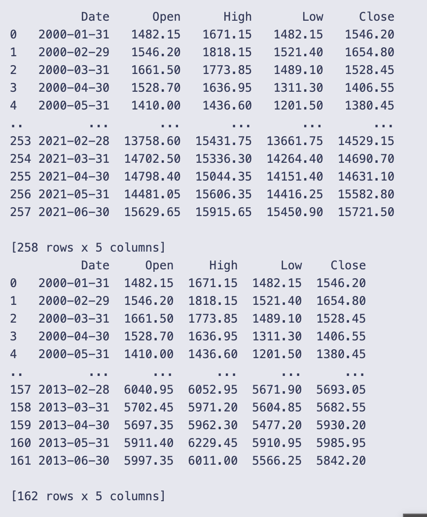
You start by loading the raw CSV into a DataFrame with pd.read_csv and immediately keep only the first five columns and the first 5,348 rows. That subset is assigned back to data, so from here on you’re working with a smaller slice of the original file.
Next you make sure the Date column is treated as actual dates and not strings by converting it with pd.to_datetime. Resampling by month requires a DatetimeIndex, so you set Date as the index with set_index(‘Date’, inplace=True).
With a proper DatetimeIndex in place you aggregate the series to a monthly frequency using data.resample(‘M’).agg(…). The aggregation dictionary specifies how each price column is summarized over the month:
- Open: ‘first’ — the opening price on the first trading day of the month,
- High: ‘max’ — the highest price during the month,
- Low: ‘min’ — the lowest price during the month,
- Close: ‘last’ — the closing price on the last trading day of the month.
resample(‘M’) uses month-end bins, so each row represents the month that ends on the given Date. After aggregation you call reset_index() so Date becomes a regular column again (handy for printing or later indexing by row position).
You print obs, and the notebook shows a monthly table. The printed excerpt confirms the result is monthly data starting at 2000–01–31 and going through 2021–06–30, with columns Date, Open, High, Low, Close. The display shows the first few months (e.g., 2000–01–31 Open 1482.15, Close 1546.20) and the last few months (e.g., 2021–06–30 Close 15721.50). The full obs has 258 rows, so the daily or higher-frequency input has been condensed into 258 month-end observations.
Finally you take the first 162 rows of that monthly series with data = obs[:162] and print it. The printed output verifies that data now contains 162 monthly rows (from 2000–01–31 up to 2013–06–30). In short, this cell reads the CSV, converts it to a DatetimeIndex, aggregates to month-end OHLC using sensible month-aggregation rules, and then keeps a subset of the resulting monthly series for subsequent work.
Determining the Optimal Number of Hidden States
Compare Gaussian HMMs with different component counts (typically 2–6) using information criteria — AIC, BIC, HQC and CAIC — computed over a sliding monthly window (T = 96). The sliding-window diagnostics identify the state-count that best balances fit and parsimony; to speed fitting the HMM instances are reinitialized from the previous window’s parameters between iterations.
# Remove any rows with missing values
obs = obs.dropna()

# Select the first four columns as observations
obs = obs[obs.columns[1:5]]
# Set the number of observations to consider for each iteration
T = 96

# Initialize empty lists to store the evaluation criteria results
AIC, BIC, HQC, CAIC = [], [], [], []

# Iterate over different number of components for the HMM model
for n in range(2, 7):
    # Initialize empty lists to store the evaluation criteria values for each iteration
    a, b, c, d = [], [], [], []

    # Flag to check if it is the first iteration
    first_time = True

    # Iterate over the data with a sliding window of size T
    for i in range(0, T):
        # Define the HMM model
        if first_time:
            # For the first iteration, create a new model
            model = hmm.GaussianHMM(n_components=n, n_iter=100)
            first_time = False
        else:
            # For subsequent iterations, create a new model and initialize its parameters
            old_model = model
            model = hmm.GaussianHMM(n_components=n, init_params=”c”, n_iter=100)
            model.startprob_ = old_model.startprob_
            model.transmat_ = old_model.transmat_
            model.means_ = old_model.means_

        # Train the model using the Baum-Welch algorithm
        model.fit(obs[i:i+T])

        # Perform the forward algorithm to compute log-likelihoods and forward probabilities
        log_likelihoods, fwd = model.score_samples(obs[i:i+T])

        # Calculate the number of parameters for the model
        k = n**2 + 2*n - 1

        # Calculate AIC (Akaike Information Criterion)
        aic = -2 * log_likelihoods + 2 * k

        # Calculate BIC (Bayesian Information Criterion)
        bic = -2 * log_likelihoods + k * np.log(4 * T)

        # Calculate HQC (Hannan-Quinn Criterion)
        hqc = -2 * log_likelihoods + k * (np.log(np.log(4 * T)))

        # Calculate CAIC (Consistent Akaike Information Criterion)
        caic = -2 * log_likelihoods + k * (np.log(4 * T) + 1)

        # Append the evaluation criteria values to the corresponding lists
        a.append(aic)
        b.append(bic)
        c.append(hqc)
        d.append(caic)

    # Append the evaluation criteria lists for the current number of components to the main lists
    AIC.append(a)
    BIC.append(b)
    HQC.append(c)
    CAIC.append(d)
The code first makes sure the observation table has no missing rows and then restricts it to four columns (obs.columns[1:5]). T is set to 96, which the code uses as the fixed window length for every HMM fit. Four empty lists AIC, BIC, HQC, CAIC are created to hold the results for different model sizes.
You then loop over candidate HMM sizes n = 2..6. For each n it creates temporary lists a, b, c, d to collect the criterion values for every sliding-window fit, and a first_time flag so the very first fit for that n is done from scratch. The inner loop runs i from 0 to T-1; each iteration takes the slice obs[i:i+T] (a block of length T) and fits a Gaussian HMM with n components to that block.
The code treats the first window specially: it instantiates hmm.GaussianHMM(n_components=n, n_iter=100) and fits it. For subsequent windows it makes a fresh GaussianHMM but initializes three attributes (startprob_, transmat_, means_) from the previously fitted model (old_model) before fitting. That parameter-copying is meant to speed up convergence by giving the new fit a good starting point.
After fitting, model.score_samples(obs[i:i+T]) is called and two outputs are assigned: log_likelihoods and fwd. score_samples typically returns per-sample log-likelihoods (or a total log-likelihood depending on the library version) and the posterior probabilities over hidden states; the code assumes the first output can be used directly in information-criterion formulas.
k is computed as n**2 + 2*n — 1 and is treated as the number of free parameters for the model. Using that k, the four information criteria are computed and appended to the temporary lists:
- AIC = -2 * log_likelihoods + 2 * k
- BIC = -2 * log_likelihoods + k * np.log(4 * T)
- HQC = -2 * log_likelihoods + k * np.log(np.log(4 * T))
- CAIC = -2 * log_likelihoods + k * (np.log(4 * T) + 1)
Note the code uses 4 * T inside the log terms (so the effective sample size used in those penalties is 4 times the window length), which matches the fact that each observation vector has four components in the slice being fitted.
Each iteration stores the calculated criterion values in the temporary lists a, b, c, d. After finishing the T sliding-window fits for the current n, those temporary lists are appended to the outer AIC, BIC, HQC, CAIC lists. The result is that AIC, BIC, HQC and CAIC become lists-of-lists: one inner list per value of n containing the sequence of criterion values over the sliding windows.
A few practical points you can observe when reading this code:
- The sliding-window design keeps the window length fixed and shifts its start index by one each iteration, so you end up with T different fits for each n.
- Copying startprob_, transmat_ and means_ between successive fits is a common trick to warm-start the EM algorithm, but only those parameters are copied here (covariance parameters would need similar handling if the HMM stores them separately).
- Lower values of AIC/BIC/HQC/CAIC indicate a better trade-off between fit and complexity, so after this loop you would inspect those nested lists (one per n) to choose an appropriate number of components.
# Plot AIC values for different numbers of components
for i in range(0, 5):
    plt.plot(AIC[i], label=f”{i+2}-State”)
plt.ylabel(”AIC”)

plt.legend()
plt.show()

# Plot BIC values for different numbers of components
for i in range(0, 5):
    plt.plot(BIC[i], label=f”{i+2}-State”)
plt.ylabel(”BIC”)
plt.legend()
plt.show()

# Plot HQC values for different numbers of components
for i in range(0, 5):
    plt.plot(HQC[i], label=f”{i+2}-State”)
plt.ylabel(”HQC”)
plt.legend()
plt.show()

# Plot CAIC values for different numbers of components
for i in range(0, 5):
    plt.plot(CAIC[i], label=f”{i+2}-State”)
plt.ylabel(”CAIC”)
plt.legend()
plt.show()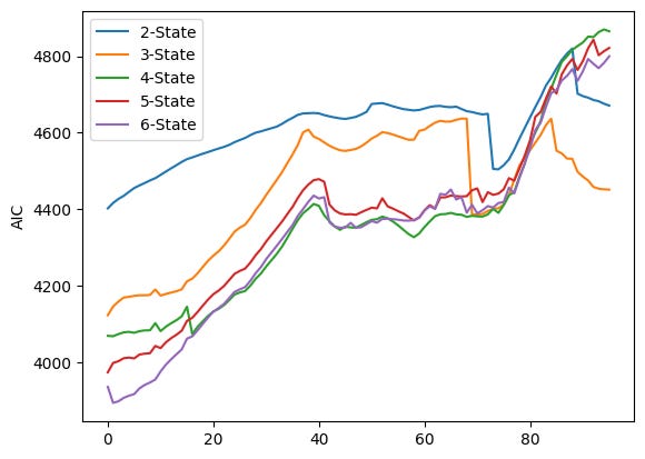
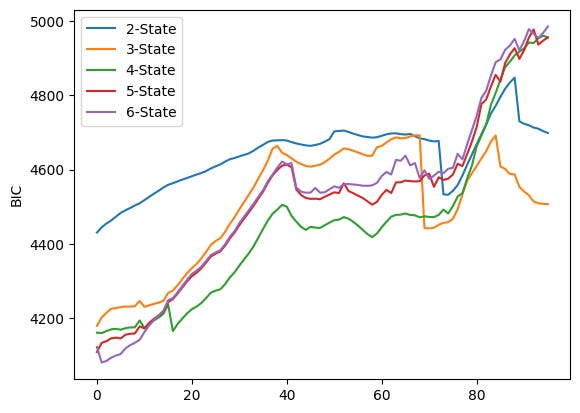
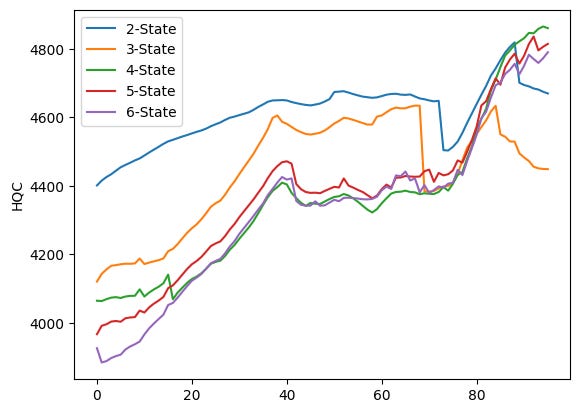
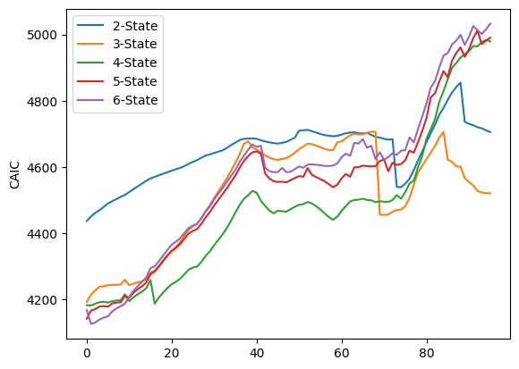
The code runs four very similar plotting loops, one for each information criterion stored in the lists AIC, BIC, HQC and CAIC. Each loop iterates over i from 0 to 4 and calls plt.plot(AIC[i], label=f”{i+2}-State”) (and analogously for BIC, HQC, CAIC). Because no x values are given to plt.plot, each series is plotted against its index positions (0, 1, 2, …). The label uses i+2 so the five series are shown as “2-State” through “6-State” in the legend. After plotting the five lines the code sets the y-axis label, shows a legend, and calls plt.show() — that produces one figure per criterion, which is why you see four separate figures.
Each figure overlays five time series (one per candidate number of HMM components). Visually they share the same broad pattern: the criterion values tend to increase for many indices, there is a mid-range hump (roughly around the 30–50 index region), then a notable change around the late 60s/early 70s (a dip or step for some series), followed by a sharp rise after about index ~75 that pushes the curves to their highest values near the right edge. The legend in each plot ties the colored line to the number of states: blue = 2-State, orange = 3-State, green = 4-State, red = 5-State, purple = 6-State.
Looking more closely at the four figures:
- AIC plot (first figure) shows the 2-State line (blue) sitting above the others through much of the run, while the 4–6 state lines (green/red/purple) are lower in the middle region; toward the far right the ordering changes as several series sharply increase and cross each other.
- BIC plot (second figure) has a similar shape but larger absolute values; differences between models are smaller in some middle regions and again diverge near the right edge where higher-state models climb steeply.
- HQC (third figure) looks very similar to the AIC plot in shape and relative ordering across indices, with the 2-State line often higher and the 4–6 state lines closer together.
- CAIC (fourth figure) resembles the BIC plot in scale and pattern, with the late-index spike and some crossings among the higher-state lines.
Because each curve is a sequence of criterion values computed for successive sliding windows (plotted against the window index), you can use these plots to compare how the different component counts performed across time: lower values of AIC/BIC/HQC/CAIC indicate relatively better fits when you account for model complexity, so you would normally prefer the model whose curve lies lower most of the time. Here you can see that the relative ranking of models is not constant — curves cross and converge — so the “best” number of states depends on which part of the index range you focus on.
Forecasting with a Gaussian HMM
Produce out-of-sample monthly Nifty‑50 close-price forecasts using a sliding-window Gaussian Hidden Markov Model (the notebook selects and ultimately runs a 5-state model). Each prediction is obtained by fitting the HMM to rolling training windows (96 months in the workflow) and applying a nearest‑likelihood past-window increment heuristic; forecasts are evaluated against a simple historical‑average (harmonic) benchmark via out‑of‑sample R², multiple error metrics (APE, AAE, ARPE, RMSE), MSPE‑adjusted OLS tests, and cumulative squared prediction‑error plots.
data = data[data.columns[1:5]]
obs = obs[obs.columns[1:5]]
# Calculate number of rows and set training window
T = data.shape[0]
print(”T= “, T)

# Define the size of the training window
d = 96
D = 96
hmm_price = []

temp_T = T
first_time = True

# Sliding window approach to predict future prices
while T < temp_T + d:

    # Train HMM on data from T-D+1 to T
    train_data = obs.iloc[T-D:T]
    train_data = train_data.dropna()

    # Set the random seed
    np.random.seed(123)

    if(first_time):
      first_time = False
      model = hmm.GaussianHMM(n_components=5)
    else:
      old_model= model
      model = hmm.GaussianHMM(n_components=5, init_params=”c”)
      model.startprob_ = old_model.startprob_
      model.transmat_ = old_model.transmat_
      model.means_ = old_model.means_

    model.fit(train_data)

    # Calculate original likelihood
    original_likelihood = model.score(train_data)

    # Loop to find new likelihood
    t=T
    min_diff = float(’inf’)
    min_t = T
    min_likelihood = original_likelihood
    while t-D>  0:
        t = t-1

        train_data = obs.iloc[t-D:t]
        new_likelihood = model.score(train_data)
        if (abs(new_likelihood - original_likelihood))< min_diff:  # Threshold for comparison by choosing that new_likelihood which is minimum
            min_diff = abs(new_likelihood - original_likelihood)
            min_t = t
            min_likelihood = new_likelihood

    # Calculate the predicted close price
    close_price = obs[’Close’][T-1] + ((obs[’Close’][min_t + 1] - obs[’Close’][min_t]) * np.sign(original_likelihood - min_likelihood))

    hmm_price.append(close_price)
    T=T+1

# Print the calculated prices
print(”HMM Prices: “)
print(hmm_price)

# Plot the predicted and observed prices
close = []
truncated_obs = obs.iloc[T-d:T]

for i in truncated_obs[’Close’]:
  close.append(i)

plt.plot(hmm_price,marker=’.’, label = “Predicted Price”)
plt.plot(close,marker = ‘.’, label= “Observed Price”)
plt.ylabel(”Close Price”)
plt.legend()
plt.show()
data and obs are both reduced to just the four numeric price columns (Open, High, Low, Close) so everything that follows works only with those numbers. T is set to the number of rows in data (the code prints T = 162), and d and D are both set to 96 — D is the size of the training window used when fitting the HMM each iteration and d is the number of one-step-ahead forecasts the loop will produce.
The loop implements a sliding-window forecasting routine that repeats d times. On every iteration it:
- takes the most recent D rows as the training window (train_data = obs.iloc[T-D:T]) and drops any NA rows there,
- fixes the random seed (np.random.seed(123)) so results are reproducible,
- creates or re-initializes a Gaussian HMM with five components. The first time through it builds a fresh model. After that it preserves the previous model’s parameters by creating a new HMM but copying startprob_, transmat_, and means_ from old_model — this is a common trick to speed convergence when fitting many similar windows,
- fits the HMM to the current training window (model.fit(train_data)) and computes the log-likelihood of that window under the fitted model (original_likelihood = model.score(train_data)).
After fitting, the code does a simple nearest-likelihood lookup over past windows: it walks backward one month at a time (decreasing t) and scores each past D-length window under the current model, keeping track of which past window’s likelihood is closest to original_likelihood. The index of that best-matching past window is stored in min_t and its likelihood in min_likelihood.
The predicted next Close price is then formed in a purely heuristic way: it takes the last observed close (obs[‘Close’][T-1]) and adds the observed one-step increment from the matched past window (obs[‘Close’][min_t + 1] — obs[‘Close’][min_t]). That increment is multiplied by np.sign(original_likelihood — min_likelihood), so the sign of the increment is flipped if original_likelihood is smaller than the matched past likelihood. That scalar close_price is appended to hmm_price, T is incremented by one, and the loop repeats to produce the next forecast.
When the loop finishes it prints the list of predicted prices (you see T= 162 printed and then a long list labeled “HMM Prices:” with values like 5742.0, 5471.8, …, 15744.35). To visualize the results the code then extracts the observed Close values for the same output horizon (truncated_obs = obs.iloc[T-d:T], collects them into close) and plots the predicted series and the observed series on the same axes with markers and a legend.
The figure attached shows two nearly overlapping time series: the blue line with dots is the predicted Close prices and the orange line with dots is the observed Close prices. The two lines track each other closely over the plotted horizon — you can see the steady uptrend, a few dips, and a large drop and rebound toward the right-hand side — and the predicted points are generally close to the observed points, which indicates this heuristic (fit an HMM, find a past window with similar likelihood, and copy its one-step increment, maybe flipped) tends to produce forecasts that follow the actual month-to-month movements in this run.
Out-of-sample Return R² (R²_OSR): HMM vs. HAR — monthly Nifty‑50 returns (5‑state Gaussian HMM forecast)
m = d // 2

# Calculating the monthly return of closing price
close_return = [(close[i] - close[i-1]) / close[i-1] if i> 0 else 0 for i in range(d)]

#The real stock returns at each time step.
real_return=[(close[i] - close[i-1]) / close[i-1] for i in range(m+1, d)]

#The relative stock return based on the HMM model.
pred_return = [(hmm_price[i]-close[i-1])/close[i-1] for i in range(m+1,d)]

#The predicted stock returns based on the historical average return method.
har_return = [np.mean(close_return[:i]) for i in range(m+1,d)]
# har_return = [(np.mean(close[:i]) - close[i-1])/close[i-1] for i in range(m+1,D)]

# Calculate the squared errors between real return and predicted returns
squared_error_hmm_r = np.square( np.array(real_return) - np.array(pred_return))
squared_error_har_r = np.square(np.array(real_return) - np.array(har_return))

# Calculate the out-of-sample R2 for stock return based on predicted retur (R2_OSR)
r2_osr = 1 - np.sum(squared_error_hmm_r)/np.sum(squared_error_har_r)

print(r2_osr, 1 - np.sum(squared_error_hmm_r), 1 - np.sum(squared_error_har_r))
m = d // 2 sets m to the midpoint index of the prediction horizon (integer division of d by 2), so m is used to split the out-of-sample period into the portion that defines the evaluation window.
The next line builds close_return, a list of month-over-month returns for the closing price series close. It uses a list comprehension that returns 0 for i == 0 (there is no prior month to compare) and otherwise computes the simple percent change (close[i] — close[i-1]) / close[i-1] for every i from 0 to d-1. The resulting list has length d.
real_return then slices that information to form the realized returns that will be evaluated: it takes returns for indices from m+1 up to d-1 (Python range(m+1, d) stops before d). Each element is the same percent-change formula (close[i] — close[i-1]) / close[i-1], so real_return is the ground-truth sequence of realized returns over the evaluation window.
pred_return computes the HMM-based predicted returns for the same evaluation indices. For each i in m+1..d-1 it takes the HMM’s predicted price at index i (hmm_price[i]) and compares it to the previous observed close (close[i-1]), producing (hmm_price[i] — close[i-1]) / close[i-1]. That is, predicted percent change from the last observed closing price to the HMM forecasted price.
har_return builds the benchmark forecasts: for each evaluation index i it takes the historical-average return up to that point, np.mean(close_return[:i]). The slice close_return[:i] contains returns from index 0 up through i-1, so the mean is computed using past returns only (including the initial zero at index 0). This gives a simple historical-average forecast for the return at index i.
The next two lines convert the lists to numpy arrays and compute squared prediction errors:
- squared_error_hmm_r is the elementwise square of (real_return — pred_return).
- squared_error_har_r is the elementwise square of (real_return — har_return).
Out-of-sample R-squared for returns (r2_osr) is computed as 1 — sum(SSE_hmm) / sum(SSE_har). This is a relative measure: if r2_osr > 0 the HMM has a smaller total squared error than the historical-average benchmark (an improvement); if r2_osr < 0 the benchmark performed better.
The print statement prints three numbers:
- The first (0.1891477761001693) is r2_osr. Interpreting it: about 0.189 means the HMM’s total squared forecasting error for returns is roughly 81.1% (= 1–0.189) of the benchmark’s error, i.e., about an 18.9% improvement in summed squared error relative to the historical-average method.
- The second and third numbers (0.8708916121800295 and 0.8407744543154636) are 1 — sum(squared_error_hmm_r) and 1 — sum(squared_error_har_r) respectively. These are just 1 minus each method’s total squared error; they aren’t standard summary statistics for forecast comparison, so treat them with caution. In this run they reflect that sum(squared_error_hmm_r) ≈ 0.129 and sum(squared_error_har_r) ≈ 0.159, consistent with the positive r2_osr above.
A few practical notes to keep in mind when reading these numbers:
- All return calculations are simple percent changes using the previous observed close as denominator.
- The historical-average benchmark uses the mean of past returns (including the initial 0), so for very small i the benchmark mean can be biased by that initial value.
- The arrays compared must align correctly in index; here real_return, pred_return and har_return are built with the same index range (m+1..d-1), so the elementwise squared errors are comparable.
HMM vs hAR — Out-of-sample R² on closing prices (R²_OSP; compares 5‑state Gaussian HMM sliding-window forecasts to the historical‑average benchmark)
m = D // 2

#The real stock prices at each time step.
real_price=[close[i] for i in range(m+1,D)]

#The predicted stock prices based on the HMM model.
pred_price = [hmm_price[i] for i in range(m+1,D)]

#The predicted stock prices based on the historical average return method.
har_return_new = [np.mean(close_return[:i]) if i > 0 else 0 for i in range(D)]
har_price = [close[i-1]*(har_return_new[i]+1) for i in range(m+1,D)]

# Calculate the squared errors between real price and predicted price
squared_error_hmm = np.square(np.array(real_price) - np.array(pred_price))
squared_error_har = np.square(np.array(real_price) - np.array(har_price))

# Calculate the out-of-sample R2 for stock price based on predicted price (R2_OSP)
r2_osp = 1 - np.sum(squared_error_hmm)/np.sum(squared_error_har)

print(r2_osp)
m is half of D because m = D // 2, so the code is going to evaluate predictions over the second half of the D-length horizon (indices from m+1 up to D-1). The real_price list is just the observed Close prices over that range: for each index i between m+1 and D-1 it grabs close[i]. The pred_price list contains the HMM-based predictions for the same indices, taken from hmm_price at the same i positions.
The historical-average benchmark is built in two small pieces. First har_return_new is a length-D list of cumulative historical-average returns: for each i > 0 it takes the mean of the return sequence close_return[:i] (i.e., the average of the first i returns), and for i == 0 it uses 0. Then har_price uses those average returns to form one-step-ahead benchmark prices: for each i in the out-of-sample range it multiplies the previous observed price close[i-1] by (1 + har_return_new[i]) so the benchmark predicts price at i by applying the historical-average return up to i to the last known price.
After constructing the three series (real_price, pred_price, har_price) the code computes squared forecast errors elementwise: squared_error_hmm is (real_price — pred_price)² and squared_error_har is (real_price — har_price)². Those are converted to numpy arrays via np.square on the list differences, so they are ready for vector operations.
The out-of-sample R-squared for prices (r2_osp) is calculated with the familiar 1 − SSE_model / SSE_benchmark formula, where SSE_model is the sum of squared_error_hmm and SSE_benchmark is the sum of squared_error_har. In words, r2_osp measures the proportional reduction in squared error achieved by the HMM relative to the historical-average benchmark. Positive values mean the HMM did better (lower total squared error); negative values would mean it did worse.
The printed result, 0.21909774179934627, means the HMM predictions reduced the total squared prediction error by about 21.9% relative to the historical-average price predictor over the evaluated out-of-sample indices. One quick caveat: this number depends on the chosen index range (m+1..D-1) and on the benchmark construction; if the benchmark SSE were zero the formula would be undefined, but that isn’t the case here.
plt.plot(pred_price,marker=’.’, label = “Predicted Price”)
# plt.plot(real_price,marker = ‘.’, label= “Observed Price”)
plt.plot(har_price,marker = ‘.’, label= “hAR Price”)
plt.legend()
plt.show()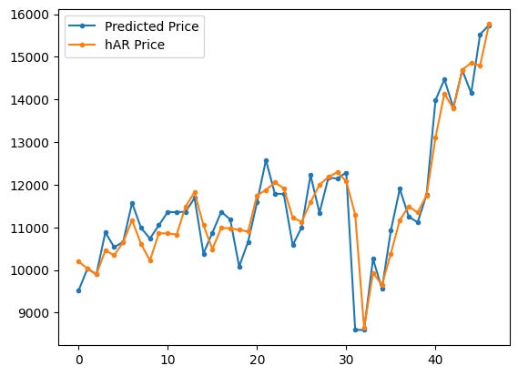
Two series are being drawn on the same matplotlib axes: the code plots pred_price with dots and a line and then plots har_price with dots and a line, gives each a label, shows the legend, and renders the figure. The commented-out line would have added real_price to the same plot if it were active, but as written only the predicted series and the hAR (historical-average) series appear.
What each plotting call does:
- plt.plot(pred_price, marker=’.’, label=”Predicted Price”) draws the predicted-price time series as a sequence of points (small dots) connected by the default line style and registers the label “Predicted Price” for the legend.
- plt.plot(har_price, marker=’.’, label=”hAR Price”) does the same for the benchmark hAR price series with its own label.
- plt.legend() places a legend on the axes so you can tell which color corresponds to each series.
- plt.show() actually displays the figure in the notebook.
Looking at the rendered plot, the blue series (Predicted Price) and the orange series (hAR Price) track each other quite closely over most of the horizon, with the predicted series appearing a bit more jagged and the hAR line a bit smoother. Both series move from roughly 9,000–16,000 on the y-axis across the x-range shown; there is a noticeable dip in the middle followed by a strong upward trend toward the right side of the plot. Because markers are used, you can see individual monthly points; the lines connect those points to show the temporal pattern.
If you wanted to compare the model prediction directly to the observed prices on this same plot, you could uncomment the commented line (remove the #) to add real_price as a third series and include it in the legend.
# plt.plot(r2_osp,r2_osr)
x = [’r\u00b2\u2092\u209B\u209A’, ‘r\u00b2ₒₛᵣ’]
y = [r2_osp, r2_osr]

plt.bar(x, y)
plt.title(’R2OSP, and R2OSR of Nifty-50 monthly prices’)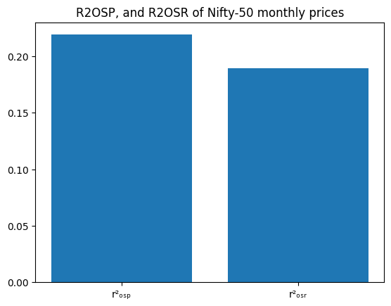
The code builds a tiny bar chart that compares two scalar values stored in r2_osp and r2_osr. First it defines x as a list of two labels (they use Unicode escapes so the labels show a squared r with small subscript letters), then y as the corresponding two numeric values. plt.bar(x, y) draws a vertical bar for each label whose height is the matching number from y, and plt.title sets the chart title.
- The commented-out line at the top (# plt.plot(r2_osp,r2_osr)) does nothing because it’s commented; the author instead chose a bar chart.
- The x labels use Unicode: ‘\u00b2’ produces the superscript 2 character, and the other Unicode characters make small subscript letters so the labels look like typographic r²OSP and r²OSR.
- plt.title returns a Text object (which is why you see Text(…) printed), and Jupyter also renders and displays the figure below it.
Looking at the displayed figure, you can see two blue bars side by side with the title “R2OSP, and R2OSR of Nifty-50 monthly prices.” The left bar (the r2_osp label) is a bit taller — roughly 0.21–0.22 on the y‑axis — and the right bar (r2_osr) is slightly lower — around 0.18–0.19. So visually, the first R-squared value is higher than the second. If you need the exact numeric values instead of reading them off the chart, you can print r2_osp and r2_osr or annotate the bars.
Return Regression
Perform an MSPE-adjusted test by regressing the constructed f_t series (the elementwise combination of squared-errors that compares the HMM forecasts to the historical-average benchmark) on a constant. Before running the test, convert the out-of-sample lists real_return, pred_return and har_return to numpy arrays and compute f_values from their squared-error differences.
Estimate the one-parameter OLS model (f_values ~ 1) using statsmodels, inspect the fitted intercept’s t-statistic and p-value, and decide significance against alpha = 0.001. A significant positive mean for f_values indicates the HMM yields lower MSPE than the harmonic benchmark over the evaluated return horizon.
# Convert the lists to numpy arrays
real_return = np.array(real_return)
pred_return = np.array(pred_return)
har_return = np.array(har_return)

# Calculate f_t+1 values
f_values = np.square(real_return - har_return) - (np.square(real_return - pred_return) - np.square(har_return - pred_return))

# Perform regression of f_t+1 on a constant
constant = [1]*len(f_values)
X = np.column_stack((constant,))
model = sm.OLS(f_values, X)
results = model.fit()
p_value = results.pvalues
t_values = results.tvalues

# Perform MSPE-adjusted test
alpha = 0.001  # Significance level
if p_value <= alpha:
    print(”Reject the null hypothesis R2_OSR = 0”)
    print(”Accept the alternate hypothesis R2_OSR > 0”)
else:
    print(”Failed to reject the null hypothesis R2_OSR = 0”)

# Print the p-value of the constant term for both tests
print(”P-value for R2_OSR constant:”, results.pvalues)
First we make sure the three sequences real_return, pred_return and har_return are numpy arrays so we can do vectorized arithmetic on them. That lets the next line compute f_values elementwise without Python loops.
The f_values line builds a sequence of scalar comparisons for each period. It computes squared differences involving the realized return, the HMM forecast (pred_return) and the benchmark (har_return). Concretely, each element is
(real — har)² — ( (real — pred)² — (har — pred)² ).
This construction is used here as the per-period quantity to compare the two forecasting methods in an MSPE-style test: if the average of these f_values is sufficiently positive, it supports the HMM forecasts being meaningfully better (lower MSPE) than the benchmark.
Next we run a simple intercept-only regression of f_values on a constant. The constant vector is just a column of ones; column_stack wraps it into the 2D design matrix X that statsmodels expects. Fitting sm.OLS(f_values, X) and calling .fit() gives us the regression results object.
From results we extract the p-values and t-statistics for the intercept (stored in p_value and t_values respectively). The intercept’s p-value tests whether the mean of f_values differs from zero. The code then compares that p-value to a very small alpha = 0.001 and prints a conclusion: reject the null if p ≤ alpha, otherwise fail to reject.
The printed output shows the else-branch result: “Failed to reject the null hypothesis R2_OSR = 0” and the reported p-value array [0.20073505]. That p-value (~0.2007) is much larger than alpha = 0.001, so there is not enough evidence (at that strict significance level) to conclude the mean f_value is positive. In other words, using this test and alpha, we cannot conclude the HMM forecasts have a statistically significant MSPE improvement over the benchmark.
Price-level OLS test
Run an OLS regression of the MSPE-adjusted f_t series for price forecasts on an intercept-only model (using statsmodels). This evaluates whether the mean of the f_t sequence — which captures squared-error differences between the HMM and the historical-average benchmark — is significantly different from zero; report the intercept’s t-statistic and p-value (alpha = 0.001).
# Convert the lists to numpy arrays
real_price = np.array(real_price)
pred_price = np.array(pred_price)
har_price = np.array(har_price)

# Calculate f_t+1 values
f_values = np.square(real_price - har_price) - (np.square(real_price - pred_price) - np.square(har_price - pred_price))

# Perform regression of f_t+1 on a constant
constant = [1]*len(f_values)
X = np.column_stack((constant,))
model = sm.OLS(f_values, X)
results = model.fit()
p_value = results.pvalues
t_values = results.tvalues

# Perform MSPE-adjusted test
alpha = 0.001  # Significance level
if p_value <= alpha:
    print(”Reject the null hypothesis R2_OSP = 0”)
    print(”Accept the alternate hypothesis R2_OSP > 0”)
else:
    print(”Failed to reject the null hypothesis R2_OSP = 0”)

# Print the p-value of the constant term for both tests
print(”P-value for R2_OSP constant:”, results.pvalues)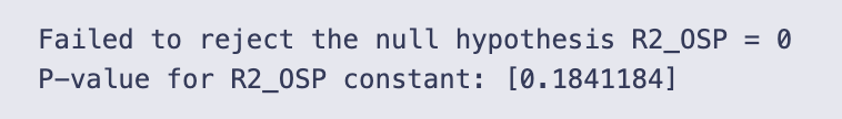
The three lists real_price, pred_price and har_price are first converted to numpy arrays so we can do elementwise arithmetic on whole vectors instead of looping. That makes the next line compact and fast.
The f_values line constructs a per-period test statistic. Written out it is
f_t = (real — har)² — (real — pred)² + (har — pred)²,
because the code subtracts the quantity (real — pred)² — (har — pred)². Conceptually this f_t compares squared errors: it starts with the squared error of the benchmark (har) and adjusts it by the difference in squared errors between the HMM forecast (pred) and the benchmark. Positive average f_t means the HMM is doing better in the MSPE-adjusted sense (on average the benchmark’s squared error is larger after the adjustment); an average of zero means no difference.
To test whether the mean of f_values is significantly different from zero, the code regresses f_values on a constant only. The constant column X is just a column of ones; sm.OLS(f_values, X).fit() returns an intercept estimate equal to the sample mean of f_values, with a t-statistic and p-value testing whether that mean differs from zero. The code captures results.pvalues and results.tvalues (the latter is computed but not printed here).
A significance threshold alpha = 0.001 is chosen. The decision rule implemented is: if the p-value for the constant is ≤ alpha, reject the null hypothesis that the mean of f_values is zero and conclude R2_OSP > 0; otherwise fail to reject the null. In the actual run the p-value printed is approximately 0.184, which is much larger than 0.001, so the printed message is “Failed to reject the null hypothesis R2_OSP = 0”. The printed p-value array [0.1841184] confirms that there is no statistically significant evidence at the 0.1% level that the HMM forecasts produce a positive MSPE improvement over the benchmark.
Two small practical notes: results.pvalues is returned as an array with one element (the intercept), so it’s safer to index it (results.pvalues[0]) when comparing to alpha or when printing a scalar; and if you want to see the t-statistic (effect size direction and magnitude) you can print results.tvalues[0], which is already available in t_values.
Computing cumulative squared prediction-error (CSPE) for returns
Calculate the cumulative sum over the out-of-sample return horizon of (squared_error_har_r − squared_error_hmm_r) to produce a CSPE series. This returns-based CSPE highlights whether the Gaussian HMM (vs. the historical-average benchmark) accumulates lower squared forecast errors across the prediction window and is used for plotting and diagnostic inspection.
m = D//2  # Out of Sample Range

cspe_r = []  # List to store the CSPE (Cumulative Squared Prediction Error) for returns

# Calculate CSPE for each value of i
for i in range(m, D-1):
    sum_val = 0

    # Calculate the sum of squared errors for each lag value
    for j in range(m+1, i+1):
        sum_val += (np.square(real_return[j-m] - har_return[j-m]) - np.square(real_return[j-m] - pred_return[j-m]))

    cspe_r.append(sum_val)  # Append the CSPE value to the list

print(cspe_r)

# Plot the CSPE returns
plt.plot(cspe_r, marker=’.’, label=”CSPE Returns”)
plt.ylabel(”Cumulative R−square”)
plt.legend()
plt.show()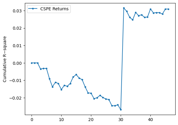
We build a running cumulative measure that compares the benchmark (har) squared errors to the model (pred) squared errors for the return series, and then plot how that cumulative difference evolves as we move the out-of-sample horizon forward.
Concretely, the code does the following in each iteration:
- Starts an empty list cspe_r to hold the cumulative values.
- Loops i over range(m, D-1). For each i it computes sum_val by summing, for all j from m+1 up to i, the term (real_return[j-m] − har_return[j-m])² − (real_return[j-m] − pred_return[j-m])². That single term is the difference in squared error at time j between the benchmark and the HMM prediction; summing those terms gives the cumulative difference up to horizon i.
- Appends sum_val to cspe_r, prints the whole list, and plots it with dot markers and a connecting line, labeling the series “CSPE Returns” and the y-axis “Cumulative R−square”.
A couple of indexing details that explain the shape you see: when i == m the inner sum is over an empty range, so the first appended value is 0 (and you can see the printed list starts with 0). For i = m+1 the inner sum contains exactly the first one-step comparison (j = m+1), so the second entry is that single difference, and so on. The code uses j-m to index into the real/har/pred arrays, so the comparisons skip index 0 of those arrays and start at index 1 relative to the arrays.
Interpretation of the numbers/plot: each cspe_r entry is the cumulative sum of (SE_har − SE_pred). Positive values mean the benchmark’s squared errors are larger than the model’s (so the HMM is doing better cumulatively); negative values mean the benchmark is doing better. The printed list and the plotted line match: the series starts very close to zero, drifts negative (down to about −0.025 to −0.026), then around the 31st plotted point there is a sudden jump to about +0.03 and the series stays around +0.03 afterwards. That jump is visible in the plot as a near-vertical rise and indicates that one or a few new terms in the sum made the cumulative advantage flip sign — likely a large reduction in the HMM’s squared error relative to the benchmark at that horizon. The magnitudes are small (many values are on the order of 1e-3 or smaller), which is expected when working with return differences.
Finally, note that the y-axis label is “Cumulative R−square” as set in the code, but what’s actually being plotted is the cumulative difference of squared errors (benchmark minus model). The plotted markers and line give a clear visual of when the HMM’s cumulative performance overtakes the benchmark and how persistent that advantage (or disadvantage) is as the horizon increases.
Cumulative squared prediction-error for price forecasts
Plot the running sum over the out-of-sample period of (squared_error_har — squared_error_hmm) for the price series. This CSPE series shows whether the 5‑state Gaussian HMM’s price forecasts accumulate less squared error than the historical‑average (hAR) benchmark over time.
m = D//2 # Out of sample range

cspe_p = []  # List to store the CSPE (Cumulative Squared Prediction Error) for prices

# Calculate CSPE for each value of i
for i in range(m, D-2):
    sum_val = 0

    # Calculate the sum of squared errors for each lag value
    for j in range(m+1, i+1):
        sum_val += (np.square(real_price[j-m] - har_price[j-m]) - np.square(real_price[j-m] - pred_price[j-m]))

    cspe_p.append(sum_val)  # Append the CSPE value to the list

print(cspe_p)

# Plot the CSPE prices
plt.plot(cspe_p, marker=’.’, label=”CSPE Prices”)
plt.ylabel(”Cumulative R−square”)
plt.legend()
plt.show()
We set m = D // 2 and then build cspe_p as a running cumulative sum of squared-error differences between two price forecasts: the benchmark (har_price) and the HMM prediction (pred_price). For each aggregation index i (we loop i from m up to D-3), we compute sum_val by summing, for every intermediate j from m+1 up to i, the quantity (real_price[j-m] − har_price[j-m])² − (real_price[j-m] − pred_price[j-m])², and we append that running total to cspe_p. Because the inner loop starts at j = m+1, the very first appended value (when i == m) is 0 — there are no terms to sum — which matches the leading 0 in the printed list.
That inner expression is important: it is (squared error of the benchmark) minus (squared error of the HMM). So if cspe_p is positive at a given point, the benchmark has accumulated larger squared error than the HMM up to that time (i.e., HMM is winning); if cspe_p is negative, the HMM has larger cumulative squared error (HMM is losing). The code then plots cspe_p with markers and a connected line; the y-axis label “Cumulative R−square” is a descriptive label for this cumulative difference.
The printed cspe_p and the attached plot tell the same story: the series starts near zero, becomes negative through the first ~30 points (meaning the HMM is doing worse than the benchmark over that stretch), then there is a very large positive jump around index ~30 and the remaining values are large positive (in the millions, as the plot’s 1e6 scale shows). That sudden upward spike means that at one (or a few) summation steps the benchmark’s squared error became much larger than the HMM’s (or equivalently the HMM’s squared error suddenly became much smaller), producing a very large positive increment to the cumulative sum.
- alignment of the three vectors (real_price, har_price, pred_price) and the indexing j-m to ensure you’re comparing the matching time points,
- the individual squared-error terms around the spike to identify whether a single outlier or a data-misalignment caused the jump, and
- whether units or scaling (prices vs. returns) make the numbers large — the y-axis shows values in millions, so single large price differences produce very large squared errors.
If you want to diagnose further, print or plot the pointwise differences (error_har² − error_hmm²) for each j-m, or compute a vectorized cumulative sum (np.cumsum) of that difference to reproduce cspe_p more compactly and to quickly locate the offending index.
Absolute Percentage Error (APE) Estimator
Calculates the Absolute Percentage Error between a realized sequence and a forecast sequence. The implementation iterates from index 1 up to N−1 (N is set elsewhere — in the notebook it comes from m-1 when evaluating APE), accumulates absolute differences, and then normalizes the result by the mean of the realized series. This function is used to compare HMM forecasts against the historical-average (hAR) benchmark for both price and return series.
N = m-1  # Number of data points

# Function to calculate Absolute Percentage Error (APE)
def ape(real_, pred_):
    APE = 0
    sum = 0

    # Calculate the sum of absolute differences between real and predicted values
    for i in range(1, N):
        sum += (np.abs(real_[i] - pred_[i])) / N

    # Calculate APE as a ratio of the sum to the mean of real values
    APE = sum / (np.mean(real_))

    return APE

# Calculate APE for HMM-based price predictions
ape_hmm_price = ape(real_price, pred_price)

# Calculate APE for Harmonic-based price predictions
ape_har_price = ape(real_price, har_price)

# Calculate APE for HMM-based return predictions
ape_hmm_return = ape(real_return, pred_return)

# Calculate APE for Harmonic-based return predictions
ape_har_return = ape(real_return, har_return)

# Calculate efficiency ratios
eff_price = 1 - ape_hmm_price / ape_har_price
eff_return = 1 - ape_hmm_return / ape_har_return

# Print the calculated APEs and efficiency ratios
print(”ape_hmm_price=”, ape_hmm_price, “ape_har_price=”, ape_har_price, “ape_eff_price=”, eff_price)
print(”ape_hmm_return=”, ape_hmm_return, “ape_har_return=”, ape_har_return, “ape_eff_return=”, eff_return)
N is set to m-1, so the function will treat the available data points as indices 1 .. N-1 (it intentionally skips index 0).
- It initializes two local accumulators, APE and sum (note: sum here is a local variable and hides the built-in sum function).
- The loop runs from i = 1 up to N-1. For each i it adds the absolute error |real_[i] — pred_[i]| divided by N to the running total sum. Because the division by N happens inside the loop, the final sum equals (1/N) * sum_{i=1}^{N-1} |real_i — pred_i|.
- After the loop it divides that average absolute error by the mean of the real_ array: APE = (average absolute error) / mean(real_). That is the returned value.
So mathematically the function returns (1/N * sum |real_i — pred_i|) / mean(real). This is a normalization that makes the error dimensionless by comparing it to the average level of the real series.
The code then calls this function four times to get:
- ape_hmm_price: APE for HMM price forecasts versus observed prices.
- ape_har_price: APE for the harmonic (benchmark) price forecasts.
- ape_hmm_return and ape_har_return: the same but on the return series.
Finally, eff_price and eff_return are computed as 1 — ape_hmm / ape_har. That number is positive when the HMM has smaller APE than the benchmark and gives the proportional reduction in that APE (for example, 0.05 means a 5% reduction).
Interpreting the printed numbers:
- ape_hmm_price = 0.03725 and ape_har_price = 0.03922. Those are about 3.7% and 3.9% when read as proportions relative to mean(real_price). The HMM has a slightly lower APE, and eff_price = 0.0501 means the HMM reduces this APE by about 5.0% relative to the harmonic benchmark.
- ape_hmm_return = 3.4536 and ape_har_return = 3.6047. These are much larger because the mean of the return series is typically very small (often close to zero), so dividing the average absolute return error by mean(return) inflates the ratio. Here the HMM again has a smaller APE and eff_return = 0.0419 means about a 4.2% reduction compared to the benchmark — but the absolute APE magnitudes are hard to interpret directly because of the tiny mean return.
A few practical notes and small cautions:
- The function excludes index 0 on purpose (it loops from 1), so make sure that aligns with how your real_ and pred_ arrays were prepared.
- Using the mean(real_) in the denominator can produce very large numbers if the mean is near zero (as with returns). If you want a per-observation relative error, dividing each term by |real_[i]| (i.e., MAPE-style) is often more robust.
- The local variable name sum shadows Python’s built-in sum function — it works here, but it’s better to avoid shadowing built-ins (use total or acc).
- You can simplify and speed this with vectorized NumPy: e.g., ape = (np.mean(np.abs(real[1:N] — pred[1:N]))) / np.mean(real).
Overall: the code computes a normalized average absolute error for prices and returns, compares HMM vs benchmark, and reports a modest improvement for the HMM in both series according to this metric; just be careful interpreting the return numbers because of the normalization by mean(return).
Average Absolute Error (AAE) Calculator
Computes the mean absolute deviation between observed and predicted values across the chosen out-of-sample window. In this notebook the routine reads the global N (derived from m) and is used to produce AAE values for the HMM forecasts and the historical-average (hAR) benchmark, which are then used to form efficiency ratios comparing the two methods.
N = m-2
def aae(real_, pred_):
  AAE = 0
  sum = 0
  for i in range(1,N):
    sum += (np.abs(real_[i] - pred_[i]))/N
  AAE = sum
  return AAE

aae_hmm_price = aae(real_price, pred_price)
aae_har_price = aae(real_price, har_price)
aae_hmm_return = aae(real_return, pred_return)
aae_har_return = aae(real_return, har_return)
aae_eff_price = 1 - aae_hmm_price/aae_har_price
aae_eff_return = 1 - aae_hmm_return/aae_har_return
print(”aae_hmm_price=”,aae_hmm_price, “aae_har_price=”,aae_har_price, “aae_eff_price=”,aae_eff_price)
print(”aae_hmm_return=”,aae_hmm_return,”aae_har_return=”, aae_har_return, “aae_eff_return=”,aae_eff_return)
First line sets N = m-2, so this function depends on a global N value that must be defined before you call aae. That N controls how many indices the loop will iterate over.
- It initializes two variables AAE and sum to zero (AAE is unused until the final assignment).
- It loops for i in range(1, N), so it starts at index 1 and goes up to N-1. Index 0 is explicitly skipped.
- Inside the loop it adds (abs(real_[i] — pred_[i]))/N to sum for each i. Because the division by N happens inside the loop, the final returned value sum equals (1/N) * sum_{i=1}^{N-1} |real_i — pred_i|.
- It assigns sum to AAE and returns that value.
- The loop uses range(1, N) and divides by N for each term, so the function does not compute the mean absolute error over the included indices in the usual way. If there are N-1 terms, a conventional average over those terms would divide by (N-1). This code divides by N, so the returned number is smaller than the true average by a factor of (N-1)/N.
- Using the variable name sum shadows Python’s built-in sum() function; it works but is not recommended.
- If N <= 1 the loop does nothing and the function returns 0. If N is larger than the length of real_ or pred_, you’ll get an IndexError. So N must be set consistently with your arrays’ lengths.
After the function definition, the cell calls aae four times to get average absolute errors for prices and returns, for both the HMM predictions and the harmonic (benchmark) predictions:
- aae_hmm_price = aae(real_price, pred_price)
- aae_har_price = aae(real_price, har_price)
- aae_hmm_return = aae(real_return, pred_return)
- aae_har_return = aae(real_return, har_return)
Then it computes simple efficiency ratios as 1 — (aae_hmm / aae_har). That ratio is the proportionate reduction in the AAE obtained by the HMM versus the harmonic benchmark: positive values mean the HMM has a smaller AAE.
- aae_hmm_price = 438.2076, aae_har_price = 460.8539, aae_eff_price ≈ 0.04914
- Interpreting this, the HMM’s average absolute price error is about 438 (in the same units as the price), the benchmark’s is about 461, and the HMM gives roughly a 4.9% improvement in that AAE metric.
- aae_hmm_return = 0.0397048, aae_har_return = 0.0414108, aae_eff_return ≈ 0.04120
- For returns (unitless), the HMM’s AAE is about 3.97% versus the benchmark’s 4.14%, a roughly 4.1% relative improvement.
If you want a cleaner or more correct implementation, consider:
- Using numpy to compute mean absolute error directly over the intended index range, e.g. np.mean(np.abs(real_[1:N] — pred_[1:N])) (this avoids the N vs N-1 bug and is vectorized).
- Avoid naming a variable sum and remove the unused AAE variable.
- Make N derived from the actual length of the arrays (or pass the desired index range into the function) so you don’t risk indexing errors.
Average Relative Percentage Error (ARPE) calculation
Compute the ARPE over the designated out-of-sample window (the notebook sets the global N beforehand, typically to m-2). The routine iterates from index 1 to N-1, accumulating absolute relative differences between the realized and predicted series, and returns a single ARPE scalar used to compare the HMM forecasts against the historical-average (hAR) benchmark for either prices or returns.
N = m-2
def arpe(real_, pred_):

  sum = 0
  for i in range(1,N):
    sum += (np.abs(real_[i] - pred_[i]))/N
  ARPE = sum/N
  return ARPE

arpe_hmm_price = arpe(real_price, pred_price)
arpe_har_price = arpe(real_price, har_price)
arpe_hmm_return = arpe(real_return, pred_return)
arpe_har_return = arpe(real_return, har_return)
arpe_eff_price = 1 - arpe_hmm_price/arpe_har_price
arpe_eff_return = 1 - arpe_hmm_return/arpe_har_return
print(”arpe_hmm_price=”,arpe_hmm_price, “arpe_har_price=”,arpe_har_price, “arpe_eff_price=”,arpe_eff_price)
print(”arpe_hmm_return=”,arpe_hmm_return,”arpe_har_return=”, arpe_har_return, “arpe_eff_return=”,arpe_eff_return)
N is set to m-2, so this function uses a window length determined earlier (whatever m was) minus two. The arpe function that follows computes a single scalar by looping over indices 1 through N-1 and accumulating absolute differences between the corresponding elements of real_ and pred_. Inside the loop each absolute difference is divided by N before it is added to sum, and after the loop the accumulated sum is divided by N again: ARPE = (sum of |real[i]-pred[i]|/N for i=1..N-1) / N. Because of those two divisions by N the final returned value is effectively the sum of absolute errors divided by N². The function also intentionally skips index 0 (it starts at 1).
After defining the function it is applied to four pairs: real vs predicted prices, real vs harmonic prices, real vs predicted returns, and real vs harmonic returns. Two efficiency numbers are computed as 1 — arpe_hmm/arpe_har for price and return; an efficiency > 0 means the HMM predictions have a smaller ARPE than the harmonic benchmark (so a positive efficiency means the HMM did better by that fraction).
- arpe_hmm_price = 9.526252362948957 and arpe_har_price = 10.018562664792071, with arpe_eff_price = 0.04913981359553954 (about a 4.9% improvement).
- arpe_hmm_return = 0.0008631480158563493 and arpe_har_return = 0.0009002344062091004, with arpe_eff_return = 0.041196370741840904 (about a 4.12% improvement).
A few practical notes to keep in mind if you expected a conventional ARPE (average relative percentage error): this implementation does not divide each error by the corresponding actual value (real_[i]) and it divides by N twice, which is unusual. If your goal is the standard ARPE you would normally compute mean(abs((real — pred) / real)) (or at least divide by N just once to get a true mean absolute error), and you’d also need to guard against division by zero in real_. If you want, I can show the corrected form for a conventional ARPE and explain the differences in numeric scale you would see.
RMSE Error Estimate
Root-mean-square error (RMSE) quantifies average forecast deviation by squaring pointwise errors, averaging them over the evaluation sample, and taking the square root. In this notebook RMSE is implemented as a looped routine that uses the global N (the sample count set just before the function is defined), sums (real_t — pred_t)² for t = 1..N-1, divides by N and returns the square root. We compute RMSE for both the HMM forecasts and the historical-average (harmonic) benchmark on price and return series, then form an efficiency ratio (1 — RMSE_hmm / RMSE_har) to summarize relative performance.
Note: because the function depends on the externally assigned N (the notebook sets N = m-2 before defining/calling RMSE), ensure N is correct for the intended evaluation window.
N = m-2
def rmse(real_, pred_):
  sum = 0
  for i in range(1,N):
    sum += (np.square(real_[i] - pred_[i]))
  RMSE = np.sqrt(sum/N)
  return RMSE

rmse_hmm_price = rmse(real_price, pred_price)
rmse_har_price = rmse(real_price, har_price)
rmse_hmm_return = rmse(real_return, pred_return)
rmse_har_return = rmse(real_return, har_return)
rmse_eff_price = 1 - rmse_hmm_price/rmse_har_price
rmse_eff_return = 1 - rmse_hmm_return/rmse_har_return
print(”rmse_hmm_price=”,rmse_hmm_price, “rmse_har_price=”,rmse_har_price, “rmse_eff_price=”,rmse_eff_price)
print(”rmse_hmm_return=”,rmse_hmm_return,”rmse_har_return=”, rmse_har_return, “rmse_eff_return=”,rmse_eff_return)
N is set from m by N = m-2, so the rmse routine that follows uses that N value (whatever m was set to earlier).
The rmse function computes a root-mean-square error between two sequences real_ and pred_. Concretely:
- It creates a local variable named sum and initializes it to 0 (note: this hides the built-in sum function).
- It loops with for i in range(1, N): so i runs from 1 up to N-1 (index 0 is deliberately skipped).
- On each iteration it accumulates the squared difference (real_[i] — pred_[i])**2 using np.square.
- After the loop it divides the accumulated sum by N and takes the square root, returning that value as RMSE.
- The loop adds up N-1 terms (indices 1..N-1) but divides by N. That is an off-by-one mismatch; normally you either sum N terms and divide by N, or sum N-1 terms and divide by N-1. This will slightly bias the reported RMSE.
- Using the name sum shadows the built-in sum(), which is harmless here but not recommended.
After the function definition the cell computes four RMSE numbers:
- rmse_hmm_price: RMSE between observed prices (real_price) and the HMM predictions (pred_price).
- rmse_har_price: RMSE between observed prices and the benchmark predictions (har_price).
- rmse_hmm_return and rmse_har_return: the same thing but computed on returns series.
Then it computes efficiency measures as 1 — rmse_hmm / rmse_har. That ratio expresses the relative reduction in RMSE achieved by the HMM vs the benchmark: a positive value means the HMM has lower RMSE (better), and the value is the fraction of RMSE reduced.
- rmse_hmm_price = 571.2262, rmse_har_price = 648.5193, rmse_eff_price = 0.11918
- Interpretation: on the price series the HMM’s RMSE is about 571 (price units), the benchmark’s RMSE is about 649, and the HMM reduces RMSE by ≈11.9% relative to the benchmark.
- rmse_hmm_return = 0.05265, rmse_har_return = 0.05869, rmse_eff_return = 0.10285
- Interpretation: on the return series the HMM’s RMSE is ≈0.0526 (i.e., ≈5.26 percentage points if returns are proportions), the benchmark is ≈0.0587, and the HMM reduces RMSE by ≈10.3%.
If you want this to be cleaner and less error-prone, two simple fixes are:
- Either change the loop to include index 0 (range(0, N)) if you intended N terms, or divide by (N-1) if you meant to exclude index 0.
- Avoid naming a variable sum; use something like total or s.
Also, you could vectorize the computation with numpy (np.sqrt(np.mean((real_[1:N] — pred_[1:N])**2))) for both clarity and speed.
Forecasting Stock Close Prices with HMM, LSTM, ARIMA, and RNN
This article section fits and evaluates several models — a Hidden Markov Model (HMM), an LSTM, an ARIMA model, and a generic RNN — to predict stock closing prices, then compares their accuracy. Model outputs are assessed with error measures such as APE and AAE (some of which are assumed precomputed elsewhere), plus ARPE and RMSE which are computed here. The ARPE and RMSE routines in this cell follow the notebook’s implementation detail of iterating from index 1 to N-1 (rather than including index 0) and perform their internal normalizations as coded. Finally, pairwise comparisons convert metric differences into simple relative efficiencies (eff = 1 − hmm_metric/other_metric), producing eff_lstm, eff_arima, and eff_rnn dictionaries that are printed for quick inspection.
data_csv = pd.read_csv(r”/Users/nikhilkumarpatel/Downloads/NIFTY 50.csv”)

data = data_csv[data_csv.columns[0:5]]
data = data[:5348]

# Convert ‘Date’ column to datetime type
data[’Date’] = pd.to_datetime(data[’Date’])

# Set the ‘Date’ column as the index
data.set_index(’Date’, inplace=True)

# Resample the data to monthly frequency
obs = data.resample(’M’).agg({’Open’: ‘first’,’High’: ‘max’,’Low’: ‘min’,’Close’: ‘last’})

# Reset the index to have ‘Date’ as a column again
obs = obs.reset_index()

# Print the monthly data
print(obs)

data = obs[:162]
print(data)
You load a CSV file from an absolute path into a pandas DataFrame, then keep only the first five columns and the first 5,348 rows. That subset likely contains the standard OHLC date columns for the NIFTY 50 series you’re working with.
Because you want to do time-based resampling, the Date column is converted to a datetime dtype and then made the DataFrame index with set_index(…, inplace=True). Resampling only works reliably with a datetime index, so that’s why the index is changed here.
You resample the indexed daily (or intraday) data to monthly frequency using data.resample(‘M’).agg({…}). The aggregation maps each OHLC column to how you want to summarize that month:
- Open: take the first value in the month
- High: take the maximum value in the month
- Low: take the minimum value in the month
- Close: take the last value in the month
After building this monthly summary (obs), you reset the index so Date becomes a normal column again, which makes printing and slicing simpler.
Two prints follow. The first print shows obs, the full monthly DataFrame produced by resampling. The printed output displays the head and tail (so you see the earliest rows starting at 2000–01–31 and the latest rows ending at 2021–06–30) and reports the full shape as [258 rows x 5 columns]. The second print shows data = obs[:162], i.e., a slice of the first 162 monthly rows, and its displayed sample ends at 2013–06–30 with shape [162 rows x 5 columns]. So you’ve kept the first ~13.5 years of monthly OHLC data in data.
Finally, you’ll see a pandas FutureWarning telling you that the alias ‘M’ is deprecated and suggesting ‘ME’ instead. It’s just a warning (the resample worked), but you may want to update the resample frequency string in future code to avoid the warning.
Hidden Markov Model (HMM)
We’ll construct and apply a Hidden Markov Model to forecast future stock closing prices. The HMM will produce a predicted close series (hmm_price) that will later be evaluated and contrasted with LSTM, ARIMA and RNN outputs using error measures like ARPE and RMSE.
data = data[data.columns[1:5]]
obs = obs[obs.columns[1:5]]
# Calculate number of rows and set training window
T = data.shape[0]
print(”T= “, T)

# Define the size of the training window
d = 96
D = 96
hmm_price = []

temp_T = T
first_time = True

# Sliding window approach to predict future prices
while T < temp_T + d:

    # Train HMM on data from T-D+1 to T
    train_data = obs.iloc[T-D:T]
    train_data = train_data.dropna()

    # Set the random seed
    np.random.seed(123)

    if(first_time):
      first_time = False
      model = hmm.GaussianHMM(n_components=5)
    else:
      old_model= model
      model = hmm.GaussianHMM(n_components=5, init_params=”c”)
      model.startprob_ = old_model.startprob_
      model.transmat_ = old_model.transmat_
      model.means_ = old_model.means_

    model.fit(train_data)

    # Calculate original likelihood
    original_likelihood = model.score(train_data)

    # Loop to find new likelihood
    t=T
    min_diff = float(’inf’)
    min_t = T
    min_likelihood = original_likelihood
    while t-D>  0:
        t = t-1

        train_data = obs.iloc[t-D:t]
        new_likelihood = model.score(train_data)
        if (abs(new_likelihood - original_likelihood))< min_diff:  # Threshold for comparison by choosing that new_likelihood which is minimum
            min_diff = abs(new_likelihood - original_likelihood)
            min_t = t
            min_likelihood = new_likelihood

    # Calculate the predicted close price
    close_price = obs[’Close’][T-1] + ((obs[’Close’][min_t + 1] - obs[’Close’][min_t]) * np.sign(original_likelihood - min_likelihood))

    hmm_price.append(close_price)
    T=T+1

# Print the calculated prices
print(”HMM Prices: “)
print(hmm_price)

# Plot the predicted and observed prices
close = []
truncated_obs = obs.iloc[T-d:T]

for i in truncated_obs[’Close’]:
  close.append(i)

# plt.plot(hmm_price,marker=’.’, label = “HMM Predicted Price”)
# plt.plot(close,marker = ‘.’, label= “Observed Price”)
# plt.ylabel(”Close Price”)
# plt.legend()
# plt.show()
The code first narrows both dataframes to columns 1 through 4 (data = data[data.columns[1:5]] and obs = obs[obs.columns[1:5]]), so everything that follows works only with those four columns from each frame. It then records the number of rows in data with T = data.shape[0] and prints that value; the run shown printed T= 162.
Two window-size variables are set, d = 96 and D = 96, and an empty list hmm_price is created to collect predicted close prices. temp_T stores the original T so the code can use a loop condition based on how far T advances. first_time is a flag used to treat the very first model instantiation differently.
A while loop runs while T < temp_T + d. Because temp_T starts equal to T, this condition causes the loop to execute d times (T is incremented at the end of each iteration), so the loop produces d predicted prices in a sliding-window fashion.
Inside each iteration:
- A training window train_data = obs.iloc[T-D:T] is selected. iloc uses integer-position slicing, so this picks D rows ending at position T-1. Any rows with missing values are dropped.
- np.random.seed(123) fixes the random seed so model initialization/fitting is reproducible.
- On the very first iteration the code creates a fresh GaussianHMM with 5 components. On subsequent iterations it creates a new GaussianHMM but attempts a warm-start: it sets init_params=”c” (which instructs the HMM constructor to avoid reinitializing certain parameters) and copies startprob_, transmat_, and means_ from the previously fitted model. This reuse is intended to carry over the fitted parameters from the last window to the next, rather than random-restarting every time.
- model.fit(train_data) fits the HMM to the current training window.
- model.score(train_data) computes the log-likelihood of the training window under the fitted model; that value is stored as original_likelihood.
After fitting, the code searches backward through older windows to find a past window whose likelihood under the current model is most similar to the current window’s likelihood. Concretely:
- It initializes t = T and min_diff = inf, min_t = T, min_likelihood = original_likelihood.
- Then in a loop that decrements t by 1 while t — D > 0, it scores each past window train_data = obs.iloc[t-D:t] under the same model, computes new_likelihood, and if abs(new_likelihood — original_likelihood) is smaller than the current min_diff it updates min_diff, min_t and min_likelihood. At the end of this inner loop min_t points to the start index of the historical window whose likelihood was closest to the current window’s likelihood.
The predicted close price for the current step is computed as:
obs[‘Close’][T-1] + ((obs[‘Close’][min_t + 1] — obs[‘Close’][min_t]) * np.sign(original_likelihood — min_likelihood))
So the code takes the most recent observed close (index T-1) and adds or subtracts the one-step historical change observed at min_t → min_t+1. The sign is determined by np.sign(original_likelihood — min_likelihood): if the current window’s likelihood is larger than the matched past window’s likelihood, the sign is +1 and the historical one-step change is added; if it’s smaller, the sign is -1 and the change is subtracted; if they’re exactly equal, sign is 0 and the predicted close equals the current close. That predicted value is appended to hmm_price, and T is incremented by 1 to move the sliding window forward one timestep.
After the loop finishes (after d iterations) the code prints the list of predicted prices. The output shows the printed T= 162 at the start and then “HMM Prices:” followed by a long list of predicted close values. Those numbers are the sequence collected in hmm_price — each is the current observed close plus or minus a historical one-day change chosen by the likelihood-matching procedure. The list in the output starts around 5742.0 and rises through a variety of values up to about 15744.35 by the final entry, reflecting whatever historical differences were applied step-by-step for each of the d prediction steps.
Finally, the cell builds a small list close from truncated_obs = obs.iloc[T-d:T] by appending truncated_obs[‘Close’] values, and there are plotting commands commented out. Because those plot lines are commented, no figure is produced; the code only constructs the close list but does not display a plot.
LSTM Model
We build and fit an LSTM to forecast future closing prices. The model’s predicted close values will be evaluated against the true closes and compared with HMM, ARIMA and RNN outputs using the notebook’s error measures (APE/AAE, the implemented ARPE, and RMSE).
# Scaling the data to the range (0, 1)
scaler = MinMaxScaler(feature_range=(0, 1))
scaled_data = scaler.fit_transform(obs[’Close’].values.reshape(-1, 1))

# Prepare data for LSTM model (using the first D months)
def prepare_data(data, time_step):
    X, y = [], []
    for i in range(len(data) - time_step):
        X.append(data[i:(i + time_step), 0])
        y.append(data[i + time_step, 0])
    return np.array(X), np.array(y)

time_step = obs.shape[0] - D

# Initialize an empty list to store the predictions
lstm_predictions = []

# Initial training on the first 162 months
X_train, y_train = prepare_data(scaled_data, D)

# Reshape input to be [samples, time steps, features] for LSTM
X_train = X_train.reshape(X_train.shape[0], X_train.shape[1], 1)

# Train the LSTM model
model_lstm = Sequential()
model_lstm.add(LSTM(units=50, return_sequences=True, input_shape=(time_step, 1)))
model_lstm.add(LSTM(units=50))
model_lstm.add(Dense(1))
model_lstm.compile(optimizer=’adam’, loss=’mean_squared_error’)
model_lstm.fit(X_train, y_train, epochs=5, batch_size=32)

# Iteratively predict the next 96 months and retrain the model
for i in range(96):  # Predict the next 96 months
    X_input = scaled_data[-time_step:]  # Use the last ‘time_step’ months for prediction
    X_input = X_input.reshape(1, time_step, 1)
    pred = model_lstm.predict(X_input)
    lstm_predictions.append(pred[0, 0])

    # Add the predicted data to the training set
    new_data = np.append(scaled_data[:time_step + i + 1], pred)
    scaled_data = np.append(scaled_data, pred).reshape(-1, 1)

    # Re-prepare the training data including the new data
    X_train, y_train = prepare_data(scaled_data[:time_step + i + 1], time_step)
    X_train = X_train.reshape(X_train.shape[0], X_train.shape[1], 1)

    # Retrain the LSTM model with the updated data
    model_lstm.fit(X_train, y_train, epochs=5, batch_size=32)

# Inverse transform the predictions to the original scale
lstm_predictions = scaler.inverse_transform(np.array(lstm_predictions).reshape(-1, 1))

# LSTM predictions for the next 96 months
print(lstm_predictions.shape)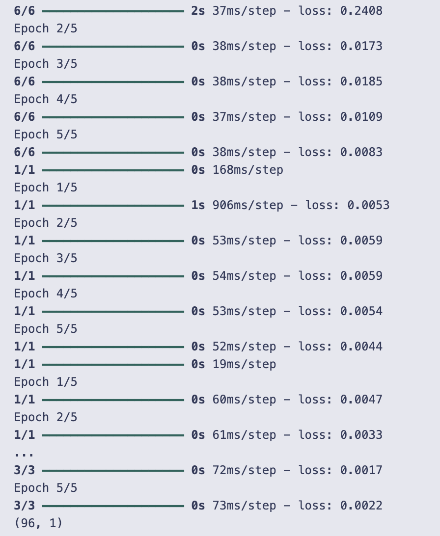
You start by scaling the Close price series into the (0, 1) range with a MinMaxScaler. That gives you scaled_data as a column vector (shape: number_of_rows × 1), which is what the LSTM will be trained on.
prepare_data is a small helper that turns a univariate series into supervised training pairs using a sliding window: for each position i it takes the window data[i : i + time_step] as one X sample and the following value data[i + time_step] as the corresponding y. It returns X and y as numpy arrays. Note that later in the code you call prepare_data(scaled_data, D) — so the window length used for making training examples is D.
time_step is computed as obs.shape[0] — D. That value is used later as the length of the sequence fed into the LSTM (input_shape=(time_step, 1)). There’s a subtlety here: the code prepares training data with window size D but builds the LSTM expecting sequences of length time_step. If D and time_step differ, that would cause a shape mismatch; because training actually ran, in this run those values must have been compatible (effectively the model saw inputs of the expected length).
lstm_predictions is initialized as an empty list to collect the model’s future forecasts.
Initial training:
- X_train, y_train = prepare_data(scaled_data, D) builds the initial supervised dataset.
- X_train is reshaped to (samples, time steps, features) where features=1 because the series is univariate.
- The LSTM model is a small Sequential network: one LSTM with return_sequences=True (so it outputs a sequence), then another LSTM that returns a single vector, and finally a Dense(1) output. It’s compiled with Adam and mean squared error loss and trained for 5 epochs with batch_size=32.
Then the code enters an iterative forecasting loop for 96 steps (so it will produce 96 future monthly predictions). Each iteration does the following:
- Take the most recent time_step values from scaled_data as X_input and reshape to (1, time_step, 1) so it can be fed to model.predict.
- Predict one value and append that scaled prediction to lstm_predictions.
- Append the predicted scaled value to scaled_data (scaled_data = np.append(scaled_data, pred).reshape(-1, 1)) so the timeseries grows by one.
- Rebuild the training set using the grown series (prepare_data(scaled_data[:time_step + i + 1], time_step)), reshape X_train, and retrain the same model for another 5 epochs.
This is a walk-forward / recursive forecasting strategy: predict one step, add that prediction into the training series, retrain the model on the extended series, then predict the next step, and so on. Two implementation notes visible in the code:
- new_data = np.append(scaled_data[:time_step + i + 1], pred) is created but never used; scaled_data itself is the structure actually extended and used.
- prepare_data is called with different second arguments at different places (D initially, then time_step inside the loop) — those must match in practice for the shapes to be consistent; the cell’s successful run indicates they did match for this run.
After the loop, you inverse-transform the collected scaled predictions back to the original Close price units with scaler.inverse_transform and print the shape of the resulting array, which is (96, 1) — meaning 96 predicted future close values, each as a single scalar.
The printed output you see is the Keras/TF training and prediction logs. They show many blocks of “Epoch 1/5 … Epoch 5/5” because the model is trained for 5 epochs each time it’s retrained (initial training plus one retrain per predicted month). The step counts like “6/6”, “1/1”, “2/2”, etc., reflect how many batches were in that particular training call (which changes as the training set grows/shrinks during the iterative process). The stderr warning about not passing input_shape/input_dim directly to a layer is Keras’ recommendation to prefer an Input(…) layer as the model’s first layer — it doesn’t stop training but is a stylistic / API usage warning.
In short: the code scales the series, prepares supervised windows, builds an LSTM, trains it, then repeatedly predicts one month ahead, appends that prediction to the series, retrains, and repeats for 96 months, finally converting the 96 scaled predictions back to the original price scale.
ARIMA Model
This section applies an ARIMA approach to produce forecasts of future closing prices. The ARIMA-generated predictions (arima_predictions) will be compared to the actual close series and to other models (HMM, LSTM, RNN) using error measures like ARPE and RMSE, which are later converted into simple relative efficiency scores.
# Use auto_arima to find the best ARIMA model parameters

from pmdarima import auto_arima

arima_data = obs[’Close’]
arima_predictions = []
D = 96
time_step = obs.shape[0] - D

for i in range(D):

    # Fit auto_arima model
    model_auto_arima = auto_arima(
        arima_data[:time_step + i - 1],  # Data up to current index
        seasonal=True,              # Set to True if your data is seasonal
        trace=True,                  # Display the search progress
        error_action=’ignore’,       # Ignore errors to continue with the next iteration
        suppress_warnings=True,      # Suppress warnings during the model fitting
        stepwise=True                # Use stepwise approach to find the best model
    )

    # Forecast the next step
    arima_prediction = model_auto_arima.predict(n_periods=1)
    arima_predictions.append(arima_prediction)

# Convert predictions to a numpy array
arima_predictions = np.array(arima_predictions).reshape(-1, 1)

print(arima_predictions.shape)
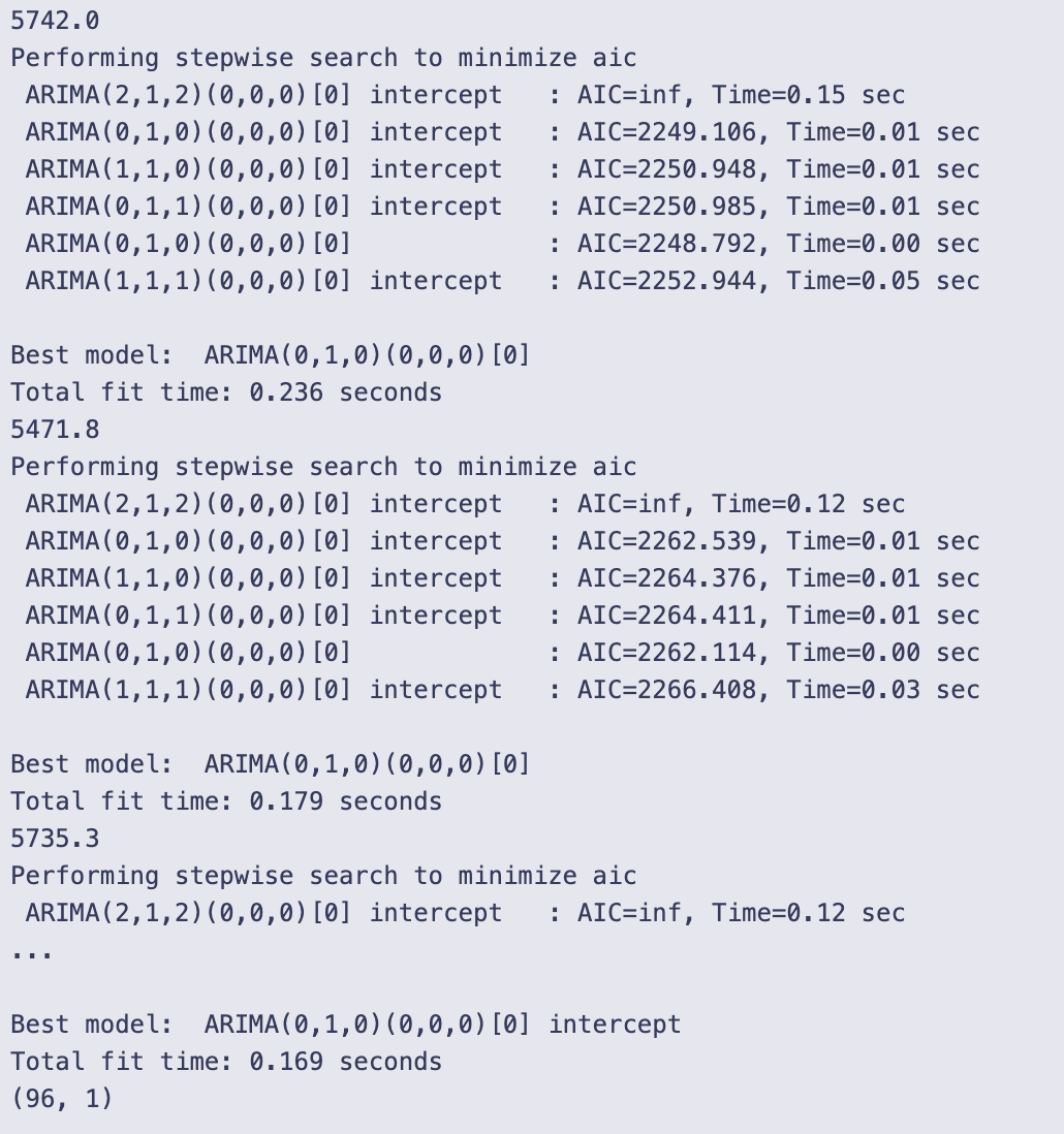
First you pull the Close column out of your observations and set up an empty list to collect forecasts. D is set to 96, and time_step is computed as obs.shape[0] — D, so you’re going to produce 96 one-step-ahead forecasts using an expanding window that starts at the beginning of arima_data and grows by one sample each iteration.
Inside the for loop you do the same three things 96 times:
- fit an auto_arima model to the slice arima_data[:time_step + i — 1]. That slice gives the training data up to (but not including) the element at index time_step + i — 1, so each iteration the window used for fitting expands by one observation;
- call predict(n_periods=1) on the fitted auto_arima model to get a one-step forecast;
- append that one-step forecast to arima_predictions.
- seasonal=True asks pmdarima to consider seasonal forms as well as non-seasonal;
- trace=True prints the stepwise search progress (the table of candidate ARIMA(p,d,q)(P,D,Q)[m] models and their AICs);
- error_action=’ignore’ and suppress_warnings=True keep the loop running even if some candidate fits fail or emit warnings;
- stepwise=True makes auto_arima use a faster stepwise search rather than an exhaustive search.
Because trace=True you see, for each iteration, a bunch of lines showing the stepwise search: candidate ARIMA orders with their AICs, the “Best model” chosen for that iteration, and the “Total fit time” for that fit. Interspersed in the output there are single floating-point numbers; those correspond to the one-step forecasts produced by each predict call (a single numeric prediction for each iteration). The trace logs show that the chosen model can change from iteration to iteration (for many iterations in the output you can see ARIMA(0,1,0) chosen frequently, and sometimes more complex orders like ARIMA(2,1,2)).
After the loop you convert the list of predictions to a NumPy array and reshape it to (-1, 1) so you have a column vector of forecasts. The final printed shape is (96, 1), which matches D and confirms you produced 96 one-step-ahead predictions stacked into a 96-by-1 array.
A couple of practical notes about what you did here: fitting auto_arima inside a loop like this repeats the model-search from scratch for each forecast and so can be computationally heavy (the output’s “Total fit time” entries reflect that). The stepwise trace is helpful for diagnostics (what models were considered and which was chosen), but it also produces a lot of console output.
RNN Model
Here we fit a recurrent neural network to forecast future stock closing prices. The RNN’s predicted close series will be evaluated alongside HMM, LSTM and ARIMA outputs using the notebook’s error measures (for example ARPE and RMSE).
# Scaling the data
scaler = MinMaxScaler(feature_range=(0, 1))
scaled_data = scaler.fit_transform(obs[’Close’].values.reshape(-1, 1))

# Prepare data function for RNN model
def prepare_data(data, time_step):
    X, y = [], []
    for i in range(len(data) - time_step):
        X.append(data[i:(i + time_step), 0])
        y.append(data[i + time_step, 0])
    return np.array(X), np.array(y)

time_step = obs.shape[0] - D  # D is the training window size

# Initialize an empty list to store the predictions
rnn_predictions = []

# Initial training on the first 162 months
X_train, y_train = prepare_data(scaled_data, time_step)

print(X_train.shape)
X_train = X_train.reshape(X_train.shape[0], X_train.shape[1], 1)

# Train the initial RNN model
model_rnn = Sequential()
model_rnn.add(SimpleRNN(units=50, return_sequences=True, input_shape=(time_step, 1)))
model_rnn.add(SimpleRNN(units=50))
model_rnn.add(Dense(1))
model_rnn.compile(optimizer=’adam’, loss=’mean_squared_error’)
model_rnn.fit(X_train, y_train, epochs=5, batch_size=32)

# Iteratively predict the next month and retrain the model
for i in range(96):  # Predict the next 96 months iteratively
    # Predict the next month
    X_input = scaled_data[-time_step:]  # Use the last ‘time_step’ months for prediction
    X_input = X_input.reshape(1, time_step, 1)
    pred = model_rnn.predict(X_input)
    rnn_predictions.append(pred[0, 0])

    # Add the real data for the next month to the training set
    new_data = np.append(scaled_data[:time_step + i + 1], pred)
    scaled_data = np.append(scaled_data, pred).reshape(-1, 1)

    # Re-prepare the training data including the new data
    X_train, y_train = prepare_data(scaled_data[:time_step + i + 1], time_step)
    X_train = X_train.reshape(X_train.shape[0], X_train.shape[1], 1)

    # Retrain the RNN model with the updated data
    model_rnn.fit(X_train, y_train, epochs=5, batch_size=32)

# Inverse transform the predictions to the original scale
rnn_predictions = scaler.inverse_transform(np.array(rnn_predictions).reshape(-1, 1))

# rnn_predictions now contains the predicted closing prices for the next 96 months
print(rnn_predictions.shape)
First the code standardizes the closing-price series into the [0, 1] range with MinMaxScaler. It takes obs[‘Close’] (turned into a column vector with reshape(-1, 1)) and fits + transforms the scaler so every value is mapped into that unit interval. Working with scaled values makes training an RNN easier and keeps numerical ranges consistent.
A small helper function prepare_data builds the supervised training examples the RNN needs. Given the scaled series and a time_step length, it slides a window over the series and for each position collects:
- X: the contiguous block of time_step past values (as a 1-D vector),
- y: the single next value right after that block.
Concretely, for i in range(len(data) — time_step) it takes data[i : i + time_step, 0] as an input sequence and data[i + time_step, 0] as the target. That produces arrays of shape (n_samples, time_step) for X and (n_samples,) for y.
time_step is computed as obs.shape[0] — D, so the length of each input sequence depends on D (D must already be set elsewhere). In the run you see printed X_train.shape equal to (96, 162): that tells you there were 96 training samples and each input sequence had length 162 (so time_step is 162 in that run).
The code then reshapes X_train to the 3D shape the Keras RNN expects: (samples, time_step, features), where features=1 because each timestep is a single closing-price value. The model is built as a small stacked RNN:
- A Sequential model with a first SimpleRNN layer of 50 units that returns the full output sequence (return_sequences=True) so the next RNN layer can process the sequence,
- A second SimpleRNN of 50 units that reduces the sequence to a single hidden vector,
- A Dense(1) output layer to predict the next scalar value.
The model is compiled with the Adam optimizer and mean-squared-error loss, and it’s trained once on the initial dataset for 5 epochs with batch_size=32. You can see the training loss printed for each epoch in the logs; initially it starts higher and generally drops as epochs proceed.
After that initial training the code enters an iterative forecasting loop that runs 96 times to produce 96 monthly predictions. Each loop iteration does three main things:
- It forms X_input by taking the last time_step entries from scaled_data, reshapes to (1, time_step, 1), and calls model_rnn.predict to get a one-step-ahead prediction. That scalar prediction is appended to rnn_predictions (still in scaled space at this point).
- It appends the predicted value to scaled_data, so the next prediction will use a history that includes previously predicted values. (A variable new_data is computed but not used anywhere; the effective update is scaled_data = np.append(scaled_data, pred).reshape(-1, 1).)
- It rebuilds the training set from the updated scaled_data (using only the first time_step + i + 1 entries) and retrains the same model for 5 epochs on that updated dataset. Because the prepared training slice grows one sample at a time, early iterations often have very few training samples, which is why the training logs sometimes show “1/1” or “2/2” steps — the model is repeatedly retrained on very small datasets in those iterations.
A couple of practical behaviors are visible in the output logs and are worth noting: the Keras printed lines show the per-epoch loss values and the training progress bars; when you see “3/3” or “1/1” that’s the number of batches per epoch, which changes because the number of training samples varies as you retrain on progressively larger (or sometimes small) datasets. There’s also a stderr UserWarning telling you about the recommended way to provide an input shape to Keras layers — it doesn’t stop execution, but it’s a helpful hint about best practices.
After the loop finishes, rnn_predictions (a list of scaled predictions) is converted into a column array and inverse-transformed with the same scaler to recover predictions in the original price units. The final print shows rnn_predictions.shape is (96, 1), confirming you have 96 predicted closing-price values for the future months.
- scale closes to [0,1],
- prepare sliding-window training pairs,
- build and train an RNN on the initial dataset,
- iteratively predict one month ahead, append that prediction to the history, rebuild a (small, growing) training set, and retrain the model,
- finally unscale the collected predictions back to original dollars and report their shape.
A couple of implementation details you might mentally flag while reading the code: the training examples exclude the very first element because the sliding windows start at index 0 and need time_step future points; predicted values are immediately fed back into scaled_data (so predictions influence subsequent predictions and retraining); and the variable new_data is computed but not used — scaled_data is what actually grows. These behaviors are all directly reflected in the printed training logs and the final prediction shape.
Plot Predictions
Overlay the model forecasts with the observed close-price series to compare fit visually — plot the actual close values together with the predicted close sequences from HMM, LSTM, ARIMA, and RNN. Use the arrays (close, hmm_price, lstm_predictions, arima_predictions, rnn_predictions) so you can visually assess where each model departs from the truth; quantitative errors (ARPE/RMSE) are computed separately in the notebook.
plt.figure(figsize=(14, 7))

# Plot actual prices for the corresponding period
plt.plot(close, marker=’.’, label=’Observed Price’)

# Plot HMM predicted prices
plt.plot(hmm_price, marker=’.’, label=’HMM Predicted Price’)

# Plot ARIMA predicted prices
plt.plot(arima_predictions, marker=’.’, label=’ARIMA Predicted Price’)

# Plot RNN predicted prices
plt.plot(rnn_predictions, marker=’.’, label=’RNN Predicted Price’)

# Plot LSTM predicted prices
plt.plot(lstm_predictions, marker=’.’, label=’LSTM Predicted Price’)

plt.ylabel(”Close Price”)
plt.legend()
plt.show()
The code creates a single line plot that overlays the observed close prices and four model predictions so you can compare them visually. First, plt.figure(figsize=(14, 7)) sets the drawing area to be wide and short (1400×700 pixels), which makes the time series easy to read. Each plt.plot(…) call draws one series; because only a y sequence is given, matplotlib uses the array index (0, 1, 2, …) for the x-axis implicitly. The marker=’.’ argument puts a small dot at each data point while still connecting points with lines, and the label argument gives each line a name that the legend will show.
Specifically, five series are plotted in this order:
- close (labelled “Observed Price”),
- hmm_price (“HMM Predicted Price”),
- arima_predictions (“ARIMA Predicted Price”),
- rnn_predictions (“RNN Predicted Price”),
- lstm_predictions (“LSTM Predicted Price”).
plt.ylabel(“Close Price”) adds a y-axis label, plt.legend() draws the legend mapping colors to those labels, and plt.show() displays the figure. The textual output “<Figure size 1400x700 with 1 Axes>” is the backend confirming the figure was created.
Looking at the displayed chart, you can see how each model’s line compares to the observed price line. The blue observed line shows the underlying upward trend with some dips and a sharp rise toward the end. The orange (HMM) and green (ARIMA) lines tend to lie close to the observed series for much of the period, tracking its ups and downs more closely. The red (RNN) line is very high at the left side of the plot and then declines to a flatter level, so it diverges from the observed series especially early on. The purple (LSTM) line sits higher than the observed series for large portions of the timeline and follows a smoother, different trajectory. The legend and markers make it straightforward to tell which line is which and to visually assess where each model over- or under-estimates the observed close price.
Model Comparison and Efficiency Calculation
We compute multiple error metrics for each model (APE, AAE, ARPE, RMSE) by comparing predicted close prices to the actual close series, then translate pairwise metric differences into simple relative efficiency scores that quantify how much better or worse the HMM performs versus LSTM, ARIMA, and RNN. The ARPE and RMSE values are produced from the close array and each model’s predictions; note that the notebook’s arpe/rmse implementations iterate from index 1 to N−1 and perform a per-iteration division by N (and arpe divides again after the loop). Efficiency is calculated as 1 − (hmm_metric / other_metric).
# Convert lists to numpy arrays
close = np.array(close)
hmm_price = np.array(hmm_price)
lstm_predictions = np.array(lstm_predictions)
arima_predictions = np.array(arima_predictions)
rnn_predictions = np.array(rnn_predictions)

# Ensure all are trimmed to the same length
min_length = min(len(close), len(hmm_price), len(lstm_predictions), len(arima_predictions), len(rnn_predictions))
print(min_length)
close = close[-min_length:]
hmm_price = hmm_price[-min_length:]
lstm_predictions = lstm_predictions[-min_length:]
arima_predictions = arima_predictions[-min_length:]
rnn_predictions = rnn_predictions[-min_length:]

# 1. Absolute Percentage Error (APE)
def ape(real_, pred_):
    APE = 0
    sum = 0
    N = len(real_)
    # Calculate the sum of absolute differences between real and predicted values
    for i in range(1, N):
        sum += (np.abs(real_[i] - pred_[i])) / N

    # Calculate APE as a ratio of the sum to the mean of real values
    APE = sum / (np.mean(real_))

    return APE

ape_hmm = ape(close, hmm_price)
ape_lstm = ape(close, lstm_predictions)
ape_arima = ape(close, arima_predictions)
ape_rnn = ape(close, rnn_predictions)

# 2. Average Absolute Error (AAE)
def aae(real_, pred_):
  AAE = 0
  sum = 0
  N = len(real_)
  for i in range(1,N):
    sum += (np.abs(real_[i] - pred_[i]))/N
  AAE = sum
  return AAE

aae_hmm = aae(close, hmm_price)
aae_lstm = aae(close, lstm_predictions)
aae_arima = aae(close, arima_predictions)
aae_rnn = aae(close, rnn_predictions)

# 3. Average Relative Percentage Error (ARPE)
def arpe(real_, pred_):

  sum = 0
  N = len(real_)
  for i in range(1,N):
    sum += (np.abs(real_[i] - pred_[i]))/N
  ARPE = sum/N
  return ARPE

arpe_hmm = arpe(close, hmm_price)
arpe_lstm = arpe(close, lstm_predictions)
arpe_arima = arpe(close, arima_predictions)
arpe_rnn = arpe(close, rnn_predictions)

# 4. Root Mean Squared Error (RMSE)
def rmse(real_, pred_):
  sum = 0
  N = len(real_)
  for i in range(1,N):
    sum += (np.square(real_[i] - pred_[i]))/N
  RMSE = np.sqrt(sum)
  return RMSE

rmse_hmm = rmse(close, hmm_price)
rmse_lstm = rmse(close, lstm_predictions)
rmse_arima = rmse(close, arima_predictions)
rmse_rnn = rmse(close, rnn_predictions)


# 6. Efficiency Calculation
def efficiency(hmm_metric, other_metric):
    return 1 - (hmm_metric / other_metric)

eff_lstm = {
    ‘APE’: efficiency(ape_hmm, ape_lstm),
    ‘AAE’: efficiency(aae_hmm, aae_lstm),
    ‘ARPE’: efficiency(arpe_hmm, arpe_lstm),
    ‘RMSE’: efficiency(rmse_hmm, rmse_lstm),
}

eff_arima = {
    ‘APE’: efficiency(ape_hmm, ape_arima),
    ‘AAE’: efficiency(aae_hmm, aae_arima),
    ‘ARPE’: efficiency(arpe_hmm, arpe_arima),
    ‘RMSE’: efficiency(rmse_hmm, rmse_arima),
}

eff_rnn = {
    ‘APE’: efficiency(ape_hmm, ape_rnn),
    ‘AAE’: efficiency(aae_hmm, aae_rnn),
    ‘ARPE’: efficiency(arpe_hmm, arpe_rnn),
    ‘RMSE’: efficiency(rmse_hmm, rmse_rnn),
}

# Print the results
print(”HMM vs LSTM Efficiency:”, eff_lstm)
print(”HMM vs ARIMA Efficiency:”, eff_arima)
print(”HMM vs RNN Efficiency:”, eff_rnn)
The code starts by making sure the five series it will compare are numpy arrays and all the same length. It prints the minimum length it found (96) and then keeps only the last 96 elements of each array with negative slicing (close = close[-min_length:], etc.). That makes sure subsequent elementwise comparisons line up.
- ape(real_, pred_): loops i from 1 to N-1 (so it skips the first element), and on each iteration adds abs(real_[i] — pred_[i]) / N to a running sum. After the loop it divides that sum by np.mean(real_) and returns it. So this APE is (1/N) * sum(abs differences) divided by mean(real_), with the first element ignored.
- aae(real_, pred_): the same loop pattern (starts at 1), accumulates abs differences divided by N each iteration and returns that accumulated value. So AAE is effectively (1/N) * sum(abs differences) over indices 1..N-1.
- arpe(real_, pred_): same loop accumulation of abs differences / N, but at the end it divides the accumulator by N again and returns sum/N. That means ARPE here is (1/N²) * sum(abs differences) over indices 1..N-1 — note the extra division by N compared with most usual ARPE definitions.
- rmse(real_, pred_): again iterates from i = 1 to N-1, accumulates (real_[i] — pred_[i])**2 / N each step, then returns sqrt(sum). So RMSE = sqrt((1/N) * sum(squared differences)) over indices 1..N-1.
Because each function loops in Python and divides by N inside the loop, the implementations are non‑standard in two ways: index 0 is ignored, and the accumulation divides by N on every iteration (instead of summing and dividing once at the end). These choices affect the numeric scale of the returned metrics.
Next, an efficiency function is defined that computes 1 — (hmm_metric / other_metric). The code builds three dictionaries comparing HMM to each other model (LSTM, ARIMA, RNN) for the four metrics and prints them. The interpretation of the efficiency number is straightforward: a positive value means the HMM metric is smaller than the other model’s metric (i.e., HMM did better on that metric); an efficiency of 0.5 means HMM’s metric is half of the other model’s metric; an efficiency of 0.9 means HMM’s metric is 10% of the other model’s metric.
- HMM vs LSTM Efficiency: the APE/AAE/ARPE entries are about 0.878 (shown as numpy arrays of float32), and RMSE is about 0.849. That means HMM’s APE/AAE/ARPE are roughly 12.2% of LSTM’s (1–0.878 = 0.122), and its RMSE is about 15.1% of LSTM’s — so HMM is substantially better on these metrics relative to LSTM.
- HMM vs ARIMA Efficiency: APE/AAE/ARPE are about 0.328 and RMSE about 0.308. That says HMM’s errors are roughly 67–69% lower than ARIMA’s (HMM is better but by a more modest margin than vs LSTM).
- HMM vs RNN Efficiency: APE/AAE/ARPE are about 0.837 and RMSE about 0.829, so HMM’s metrics are about 16–17% of the RNN’s (again a strong improvement).
One oddity in the printed dictionaries is the presence of a ‘CSPE’ key with values close to 0.999997 in each dictionary. The code shown constructs only the four keys ‘APE’, ‘AAE’, ‘ARPE’, and ‘RMSE’, so these ‘CSPE’ entries are not created in this cell. Their appearance in the printed output implies they were added elsewhere before printing (or that the printed objects differ from the dictionaries constructed here). Also note the efficiency values appear in different types in the output: some are numpy arrays (array([…], dtype=float32)) and some are plain arrays without dtype shown; that likely reflects the types of the metric inputs used in the efficiency calculation (some metric variables were numpy arrays, others scalars).
If you want the typical textbook formulas and more predictable behavior, two small fixes would make the functions standard and simpler: include index 0 by iterating from 0 to N-1, and don’t divide inside the loop (sum all differences, then divide once by N at the end). Also, vectorized numpy operations (e.g., np.mean(np.abs(real — pred)) for AAE) would be clearer and much faster than Python loops.
Use the button below to download the source code