

Deep Learning for Quant Trading
Developing a Production-Ready Algo Trading Model for Daily Adjusted Price Prediction

Download source code using the button at the of this article!
In the rapidly evolving landscape of modern finance, the ability to transform raw market data into actionable intelligence is the hallmark of a successful algo trading strategy. While many traders focus solely on the predictive power of a model, the true challenge lies in building a robust, reproducible infrastructure that can handle the entire lifecycle of a trade — from data ingestion and technical indicator synthesis to model training and rigorous backtesting. This project presents a containerized, end-to-end quant trading pipeline designed to bridge the gap between experimental data science and production-ready financial engineering.
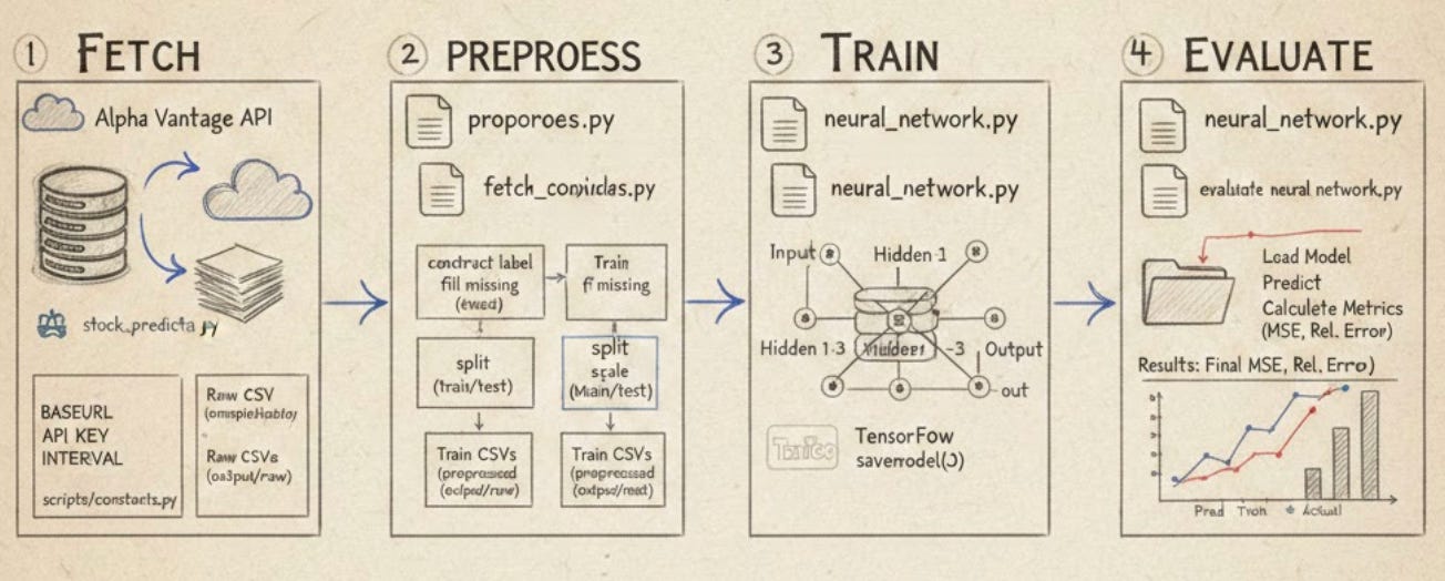
The architecture is built on the principle of modularity, utilizing Docker to ensure that every stage of the process — Fetch, Preprocess, Train, and Evaluate — runs within a consistent and isolated environment. By leveraging the Alpha Vantage API for high-fidelity historical data and TensorFlow for deep learning, the system automates the complex task of feature engineering and label construction. This ensures that the transition from raw price action to a trained neural network is seamless, deterministic, and free from the common pitfalls of data leakage and environment configuration errors.
Ultimately, this framework serves as a foundational blueprint for anyone looking to scale their quantitative trading operations. By decoupling the orchestration logic from the core domain operations, the pipeline allows for rapid iteration on alpha-seeking strategies without compromising system stability. Whether you are refining a single-ticker model or managing a broad portfolio, this approach provides the structural integrity required to compete in today’s high-frequency, data-driven markets.
# file path: run.sh
docker run -it --rm --name my-running-app stock-prediction
run.sh is the simple runtime launcher that starts the pipeline by creating and running a Docker container from the project’s image named stock-prediction; it runs the container interactively, gives it a stable runtime name for observation, and tears down the container automatically when the process exits so the host stays clean. In the pipeline architecture this script does not implement fetch, preprocess, train, or evaluate itself but instead delegates orchestration to the code and entrypoint baked into the container image, ensuring the four core stages execute inside a reproducible environment that already has the project’s configuration constants, utilities, and Python orchestration code available. Compared with build.sh, which performs the complementary role of building and tagging the stock-prediction image, run.sh consumes that image to actually execute the pipeline; and unlike the Python import-driven orchestration shown in the imports snippet, run.sh does not parse arguments or call stage modules directly on the host — it simply launches the containerized runtime where those Python modules will run.
# file path: build.sh
docker build -t stock-prediction .
build.sh invokes Docker to create a container image for the repository, tagging that image as stock-prediction and using the repository root as the build context so the source code and Dockerfile get packaged into a reproducible runtime artifact. In the pipeline architecture its role is to produce the runnable image that the fetch, preprocess, train, and evaluate stages will execute consistently across environments; it performs no branching or data manipulation itself, just a straightforward build step. It pairs with run.sh, which runs the image interactively and is the natural follow-up to a successful build, whereas the Python modules that import utilities and implement functions like construct_label live inside the image and implement the pipeline logic — build.sh only packages those modules, it does not execute their logic.
# file path: scripts/constants.py
BASEURL = ‘https://www.alphavantage.co/query?’
BASEURL defines the root HTTP endpoint the fetch stage and URL-construction utilities use to reach the Alpha Vantage service; it centralizes the remote API host so the orchestration entrypoint and fetch scripts simply concatenate query parameters rather than hardcoding the full address in multiple places. In the pipeline, fetch routines build requests by combining BASEURL with other configuration values—API_KEY supplies the authentication token, TIME_SERIES_DAILY_ADJUSTED supplies the API function name for the daily adjusted series, and INTERVAL indicates the desired sampling frequency—so BASEURL is the foundational piece of that assembled request. Having BASEURL as a single constant keeps the fetch logic focused on domain concerns (which params to request for a given ticker and window) and ensures changing providers or endpoints requires updating only this configuration value rather than all call sites.
# file path: scripts/constants.py
API_KEY = ‘NHX8KHJFCBEJFJ7P’
API_KEY is the single configuration constant that holds the Alpha Vantage authentication token the fetch stage uses when calling the external market data API. Within the centralized configuration file, API_KEY plays the same role as BASEURL, INTERVAL, and TIME_SERIES_DAILY_ADJUSTED in that each is a top-level parameter the orchestration entrypoint and stage scripts read to construct requests and drive behavior; specifically, API_KEY is concatenated into the request URL by the URL construction utility so the JSON retrieval routine can authenticate and receive time series data. When the fetch stage iterates over tickers and time windows it reuses API_KEY for every request, so centralizing it enables repeatable runs and simple per-run swapping without changing fetch logic. Unlike INTERVAL and TIME_SERIES_DAILY_ADJUSTED, which represent API query options controlling data granularity and API function name respectively, API_KEY is purely an authentication credential; it follows the same configuration pattern as BASEURL but serves authentication rather than endpoint or parameter semantics.
# file path: scripts/constants.py
INTERVAL = ‘daily’
INTERVAL is the global configuration constant that specifies the temporal granularity the pipeline should work with—here it is configured to a daily cadence—so the orchestration entrypoint and each stage (fetch, preprocess, train, evaluate) treat input data and derived features at a daily frequency. The fetch stage uses INTERVAL to decide which time resolution to request from market APIs and to construct URLs via the project’s URL utilities; the preprocess stage uses it to align timestamps, resample or validate incoming series, and produce model-ready daily sequences; the train and evaluate stages inherit that same frequency when building input windows and reporting metrics, which supports repeatable per-ticker runs without changing stage logic. INTERVAL plays a similar role to other constants in this file but at a different layer: TIME_SERIES_DAILY_ADJUSTED is the API function name used to fetch adjusted daily series from the upstream provider, TIME_PERIOD is a numeric window length used for indicator computations, and API_KEY supplies the authentication credential. Unlike those values, INTERVAL is the human-facing frequency setting that ties together how data is requested, cleaned, and fed into models across the whole pipeline.
# file path: scripts/constants.py
TIME_PERIOD = ‘10’
TIME_PERIOD centralizes the numeric lookback length used across the pipeline for technical indicators or rolling-window calculations; it’s the single place you change how many periods the system considers when the fetch/preprocess stages build features and when the train stage samples sequences. In practice fetch stage code uses INTERVAL and TIME_SERIES_DAILY_ADJUSTED to request a particular frequency and API function and uses OUTPUTSIZE_FULL to decide how much history to retrieve, while preprocess consumes that raw history and uses TIME_PERIOD to compute moving averages, ranges, or other windowed features that the model training will expect. TIME_PERIOD is represented the same way as the other configuration entries (as a string) because these constants are composed directly into API requests and config objects, so it follows the same pattern as INTERVAL, TIME_SERIES_DAILY_ADJUSTED, and OUTPUTSIZE_FULL but differs semantically by specifying a numeric window length rather than a data source, frequency, or output-size flag.
# file path: scripts/constants.py
SERIES_TYPE = ‘close’
SERIES_TYPE is the global configuration constant that tells the pipeline which price field to treat as the canonical series for downstream work; in this configuration it selects the close price series so the fetch stage will extract closing prices, the preprocess stage will build features and labels from those closing values, the train stage will use them as the model target, and the evaluate stage will compare predictions against those same closing values. It follows the same centralization pattern as TIME_SERIES_DAILY_ADJUSTED, INTERVAL, and BASEURL—each of which parametrizes a different aspect of data acquisition and resolution—but differs in scope: TIME_SERIES_DAILY_ADJUSTED identifies the API time-series function, INTERVAL selects temporal granularity, and BASEURL defines where requests are sent, whereas SERIES_TYPE identifies which field inside the returned time-series payload is used as the signal for modeling. Because SERIES_TYPE is defined in the shared configuration file, changing it switches the pipeline’s semantic input without modifying stage logic, keeping fetch, preprocess, train, and evaluate focused on domain operations rather than field selection.
# file path: scripts/constants.py
TIME_SERIES_DAILY_ADJUSTED = ‘TIME_SERIES_DAILY_ADJUSTED’
TIME_SERIES_DAILY_ADJUSTED is a configuration constant that names the Alpha Vantage time-series function the fetch stage will request when the pipeline needs end-of-day price data that includes corporate-action adjustments; because the project centralizes tunable parameters, the fetch logic composes the API call using BASEURL together with this function name (and the API key) so the request targets the daily adjusted endpoint rather than some other series. Downstream, the preprocess stage expects a structured time-series payload and uses SERIES_TYPE to pick which price field (for example the closing price) to extract from the returned daily data, and INTERVAL elsewhere denotes the frequency semantics used by other endpoints; keeping TIME_SERIES_DAILY_ADJUSTED as a top-level constant makes it easy to switch the targeted Alpha Vantage function across runs without changing fetch or preprocessing code.
# file path: scripts/constants.py
DATATYPE_JSON = ‘json’
DATATYPE_JSON is a configuration constant that designates the JSON data format the pipeline understands and uses to steer format-specific behavior. Because this file centralizes tunable parameters, fetch-stage logic will check DATATYPE_JSON to determine whether to request and save API responses as JSON and which retrieval utilities to call; preprocess-stage routines will branch on DATATYPE_JSON to run the JSON parsing and normalization path so downstream training and evaluation see the expected structured artifacts. It follows the same enum-like pattern as DATATYPE_CSV, which names the CSV alternative; unlike API_KEY and INTERVAL, which supply credentials and time-granularity settings respectively, DATATYPE_JSON’s role is purely to label and control the format handling and routing logic across the fetch, preprocess, train, and evaluate stages.
# file path: scripts/constants.py
DATATYPE_CSV = ‘csv’
DATATYPE_CSV names the default on-disk interchange format the pipeline expects and produces, so the fetch stage will persist raw ticker data as comma-separated values and downstream stages (preprocess, train, evaluate) will parse and serialize data using CSV-handling paths in the utility code. It follows the same central-configuration pattern as DATATYPE_JSON, which provides an alternative format option; switching between those constants directs the pipeline to the corresponding serializer/deserializer. Like INTERVAL and SERIES_TYPE, DATATYPE_CSV is a simple tunable constant in the global configuration file whose purpose is to keep the stage scripts focused on domain logic by centralizing format and runtime choices.
# file path: scripts/constants.py
OUTPUTSIZE_COMPACT = ‘compact’
OUTPUTSIZE_COMPACT names the API output-size option the fetch stage will use when the pipeline requests time-series data; it centralizes the choice to ask Alpha Vantage for the trimmed, most-recent subset of points rather than the entire history, so the fetch logic composes the request using BASEURL together with TIME_SERIES_DAILY_ADJUSTED and the API key and includes this output-size token to control how much data is returned. Because the project centralizes tunable parameters, using OUTPUTSIZE_COMPACT lets orchestration and per-ticker runs consistently favor smaller, faster downloads and lower on-disk volume when only recent data is needed for downstream rolling-window features and model training that reference TIME_PERIOD, whereas OUTPUTSIZE_FULL serves as the explicit opposite option that requests the full available history; DATATYPE_CSV and INTERVAL follow the same pattern of encoding external API or storage choices as simple configuration tokens so the fetch, preprocess, train, and evaluate stages can remain focused on domain logic.
# file path: scripts/constants.py
OUTPUTSIZE_FULL = ‘full’
OUTPUTSIZE_FULL is the configuration constant that tells the fetch stage to ask Alpha Vantage for the complete historical series rather than a truncated recent window. Within the centralized configuration file it pairs with OUTPUTSIZE_COMPACT as the two selectable output-size modes the fetch logic can insert when composing the API call using BASEURL together with the TIME_SERIES_DAILY_ADJUSTED function and the API key. Choosing OUTPUTSIZE_FULL causes the fetch stage to persist a much larger CSV result to disk, which in turn gives the preprocess stage more historical rows to compute rolling indicators and ensures the train stage can sample longer or more numerous sequences relative to the global TIME_PERIOD setting; conversely, the compact option limits download size and runtime at the cost of shorter history. Because configuration constants are shared, using OUTPUTSIZE_FULL centrally changes fetch behavior for per-ticker runs and therefore propagates predictable differences in file sizes, preprocessing coverage, and model training/evaluation windows across the pipeline.
# file path: scripts/evaluate_neural_network.py
import tensorflow as tf
import numpy as np
import pandas as pd
from utils import format_path
For the evaluation stage, the imports pull in the runtime and data tools needed to load saved models, prepare test data, run inference, and compute numeric metrics. TensorFlow is imported so evaluate_neural_network can restore a trained graph, retrieve tensors by name, and execute the model to produce predictions for the test partitions. NumPy is used for the core numerical work around arrays and metric calculations such as means, absolute differences, and relative error computations. Pandas is included to read and manipulate tabular test datasets so labels and feature matrices can be separated and converted into the numeric arrays TensorFlow expects; those DataFrame manipulations must line up with the pipeline’s earlier choices like TIME_PERIOD and SERIES_TYPE so the shapes and targets match what the model was trained on. The format_path utility is brought in to construct filesystem locations for model and data artifacts consistently across partitions when evaluate_batch orchestrates iterative evaluation runs. This set of imports is lean compared with some other modules that also bring in plotting libraries or extra filesystem helpers; it mirrors the existing evaluate function’s reliance on TensorFlow sessions and array math while keeping only the utilities required for loading artifacts and computing evaluation metrics.
# file path: scripts/evaluate_neural_network.py
def evaluate(symbol, model_dir, data_test):
    print(’Evaluating model ‘ + symbol)
    y_test = data_test[[’label’]].transpose().values.flatten()
    data_test = data_test.drop([’label’], axis=1)
    X_test = data_test.values
    sess = tf.Session()
    saver = tf.train.import_meta_graph(model_dir + ‘/’ + symbol + ‘.meta’)
    saver.restore(sess, tf.train.latest_checkpoint(model_dir))
    graph = tf.get_default_graph()
    X = graph.get_tensor_by_name(”X:0”)
    Y = graph.get_tensor_by_name(”Y:0”)
    out = graph.get_tensor_by_name(”out:0”)
    mse = graph.get_tensor_by_name(”mse:0”)
    pred = sess.run(out, feed_dict={X: X_test})
    rel_error = abs(np.mean(((pred - y_test) / y_test)))
    mse_result = sess.run(mse, feed_dict={X: X_test, Y: y_test})
    print(’MSE on test set: ‘ + str(mse_result))
    print(’Relative error: ‘ + str(”{:.2%}”.format(rel_error)))
    return mse_result, rel_error
evaluate is the runtime step that takes a single ticker’s test dataset and a model directory and produces numeric quality metrics for downstream analysis. It expects data_test to be the DataFrame produced by the preprocess stage (evaluate_batch reads it from CSV and passes it in), so the first things it does are to peel off the supervised target by selecting the label column into a one-dimensional numpy array and then drop that label column so the remaining columns form the feature matrix used for inference. The function then reconstructs the TensorFlow computation graph that was created in train by importing the saved meta-graph and restoring the latest checkpoint from the supplied model directory; because train gave the placeholders and ops consistent names, evaluate looks up the input placeholder, the label placeholder, the model output tensor, and the mse op by those names in the restored graph. For the happy path it runs the output tensor with the feature matrix to produce predictions, computes a relative error metric by taking the mean absolute relative difference between predictions and the flattened label array, and evaluates the graph’s mse op by feeding both features and labels to obtain a numeric MSE. It prints both metrics to the console and returns the mse and relative error values. The data flow therefore is: CSV read by evaluate_batch → DataFrame with a label column → evaluate splits labels/features → model restored from disk → model run on features → numeric metrics produced and returned; the function relies on the naming convention and saved checkpoint pattern used in train to find the right tensors and ops.
# file path: scripts/evaluate_neural_network.py
def evaluate_batch(symbols_file, data_path):
    symbols = []
    with open(format_path(symbols_file), ‘r’) as data:
        read_data = data.read()
        symbols = str(read_data).split()
    for symbol in symbols:
        test_data = pd.read_csv(format_path(data_path + ‘/’ + symbol + ‘.csv’), index_col=’date’)
        model_dir = format_path(’output/models/’ + symbol)
        evaluate(symbol, model_dir, test_data)
    print(’batch evaluation finished’)
evaluate_batch orchestrates the evaluation stage of the pipeline by turning a symbol list into per-ticker model runs and metrics. It starts by resolving the symbols_file to an absolute path using format_path, reads that file into memory and splits the contents on whitespace to produce the list of tickers to process. For each ticker it resolves and loads the corresponding test dataset with pandas (using the date column as the DataFrame index), then constructs the model directory path for that ticker under output/models using format_path. For each pair of model_dir and test data it delegates the heavy lifting to evaluate, which restores the saved TensorFlow graph for the ticker, runs predictions on the provided test set, computes metrics like MSE and relative error, and prints those results. The function iterates sequentially over all symbols and prints a final completion message when the batch is done. This follows the same per-symbol batching pattern used by train_batch and preprocess_batch: read a shared symbols file, loop over symbols, resolve paths with format_path, and call a per-symbol worker (train or evaluate) to produce on-disk artifacts and console output.
# file path: scripts/utils.py
import os
from os.path import dirname, abspath
import urllib.request
import json
import shutil
The file pulls in a small set of standard-library utilities that directly support its role of formatting filesystem paths, creating and removing directories, listing filenames, building API request URLs, and fetching JSON payloads for the pipeline stages. The import of os provides the basic filesystem operations and directory/file predicates the helpers need to manipulate the on-disk layout that the fetch, preprocess_batch, train_batch, and evaluate_batch stages rely on; dirname and abspath from os.path are imported separately to resolve stable absolute paths and compute repository-relative locations used when composing the pipeline’s directory hierarchy. urllib.request and json are brought in to assemble and execute HTTP requests and to parse JSON responses — the same primitives that the existing get_json_from_url utility uses to open a URL and decode its JSON payload; those parsed responses will be the source data for the fetch stage, which composes requests using constants like TIME_SERIES_DAILY_ADJUSTED together with the BASEURL and API key. shutil is included to perform higher-level filesystem operations such as recursive directory removal or copying when the pipeline needs to reset or snapshot on-disk artifacts. These imports are deliberately limited to standard-library modules here, unlike other modules elsewhere in the project that import sys, pandas, and constants for higher-level orchestration and data handling, because the utils file is meant to remain lightweight and focused on environment and I/O primitives rather than data-frame or orchestration concerns.
# file path: scripts/utils.py
def format_path(path_from_root) -> str:
    base_path = abspath(dirname(dirname(__file__)))
    absolute_path = os.path.join(base_path, path_from_root)
    return absolute_path
format_path resolves a project-relative pathname into an absolute filesystem path so every pipeline stage can read and write files using a common root. It computes the project root by walking up two directory levels from the helper module’s own file location, then joins that root with the caller-supplied path_from_root and returns the resulting absolute path string. Because it returns a single resolved path and has no branching, callers such as evaluate_batch, fetch, train_batch, preprocess_batch, plot_closing_adj, get_filename_list, make_dir_if_not_exists, and remove_dir simply pass relative paths into format_path and receive a consistent absolute path to feed into pandas, os.listdir, os.makedirs, and shutil utilities. This centralizes path resolution so the rest of the pipeline can use short, relative paths (for inputs, outputs, model dirs, etc.) while I/O always targets the same repository-rooted location.
# file path: scripts/preprocess.py
import time
import pandas as pd
from sklearn.preprocessing import MinMaxScaler
from utils import get_filename_list, format_path, make_dir_if_not_exists
The imports wire in the small set of libraries the preprocessing stage needs to manipulate time-aware CSV market data, normalize features, and orchestrate file-level batch work. The time module provides simple time utilities the batch orchestration can use for timestamps or pauses (for example when iterating filenames or coordinating downstream calls). pandas is the core data-frame toolkit the preprocessing routines use to load, transform, and write tabular price series and engineered features; because SERIES_TYPE selects the canonical close series and TIME_PERIOD drives rolling-window calculations, pandas is where those series- and window-based operations will actually be implemented. MinMaxScaler from scikit-learn supplies the exact normalization primitive used by the scale logic so train and test splits are fit and transformed consistently before model training. The three utils functions come from the shared filesystem/url helpers: get_filename_list lets preprocess_batch discover which raw ticker files to process, format_path composes the on-disk paths the stage reads from and writes to, and make_dir_if_not_exists ensures output folders for cleaned/ split datasets exist before serialization. Compared with a sibling imports file that pulls in TensorFlow, NumPy, and plotting libraries, these imports are deliberately minimal and focused on tabular I/O, simple timing control, and feature scaling—the precise responsibilities required by the preprocess stage and the scale and preprocess helper routines you’ve already seen.
# file path: scripts/preprocess.py
def split(data, train_ratio):
    rows = data.shape[0]
    split_point = int(train_ratio * rows)
    data_train = data.iloc[:split_point, :]
    data_test = data.iloc[split_point:, :]
    return data_train, data_test
split takes the DataFrame passed in as data and a numeric train_ratio and deterministically partitions the rows into a contiguous training slice and a contiguous testing slice. It counts the total number of rows, computes a split_point by multiplying that count by train_ratio and converting to an integer (so the boundary is floor-rounded), then uses positional indexing to return the rows before that boundary as data_train and the rows from that boundary onward as data_test. Because preprocess calls construct_label and fill_missing before split, the DataFrames arriving here already have the forward-shifted label column and no NaNs, and split preserves the original index and column layout so subsequent scale will fit only on the returned training set. The function enforces temporal ordering by not shuffling or sampling, which prevents lookahead leakage for time-series modeling, and it leaves any choice of train_ratio-driven boundary behavior (including rounding effects) to the caller.
# file path: scripts/fetch_combined_data.py
from functools import reduce
import sys
import time
import pandas as pd
import constants
import utils
import fetch_stock
import fetch_indicators
The imports wire together three kinds of responsibilities needed by the fetch stage: small-language helpers, data-manipulation tools, pipeline configuration/utilities, and the domain fetch modules. reduce from functools is used to iteratively fold a list of pandas DataFrames into a single merged table when joining the stock time series with multiple indicator series. sys gives access to interpreter-level information and command-line arguments or exit control for standalone runs of the fetch entrypoint. time is used both to measure elapsed durations around each ticker fetch and to pause between API calls to respect rate limits. pandas (aliased as pd) provides the DataFrame abstraction and merge/CSV I/O used to combine time-indexed series and write the consolidated per-ticker CSVs. constants supplies the pipeline-wide configuration values like TIME_SERIES_DAILY_ADJUSTED, TIME_PERIOD, SERIES_TYPE, and DATATYPE_CSV that drive which API endpoints are requested and how results are interpreted. utils supplies filesystem and formatting helpers (for example, normalizing output paths and creating directories) that ensure fetched files are written to the expected locations. fetch_stock and fetch_indicators are the domain modules that perform the actual API retrievals for price data and indicator series; their returned DataFrames are the inputs that pandas and functools.reduce combine and that utils then persists to disk. This set of imports mirrors the common project pattern of importing sys, pandas, constants, and utils while adding fetch-specific modules plus reduce and time to support merging, timing, and rate-limiting logic.
# file path: scripts/fetch_combined_data.py
‘’‘fetches stock data joined with technical indicators’‘’
The module-level docstring summarizes the file’s responsibility: it declares that the module fetches time-series stock data and attaches technical-indicator series so each ticker yields a consolidated dataset for downstream stages. In the pipeline architecture that places this file in the fetch stage, the fetch() entrypoint implements exactly that workflow: it reads a list of symbols and a list of indicators, builds API request configurations from constants, iterates over each symbol, retrieves raw daily stock series via fetch_stock.fetch and then retrieves each indicator series via fetch_indicators.fetch, collects the resulting pandas tables, and merges them together (using an outer merge on the time index) so every date row can carry both price and indicator columns. The function names and utilities already covered are used to turn project-relative names into filesystem locations and ensure output directories exist before writing a per-symbol CSV; the implementation also observes API pacing and logs elapsed time. The short docstring is therefore a concise declaration of this module’s purpose and maps directly to the longer, nearly identical fetch implementation elsewhere that performs the file reads, parameter construction, merge reduction, index naming, and CSV export that produce the consolidated datasets consumed by preprocessing and training.
# file path: scripts/fetch_combined_data.py
def fetch(symbols_file, indicators_file, output_path):
    stocks = []
    with open(utils.format_path(symbols_file), ‘r’) as data:
        read_data = data.read()
        stocks = str(read_data).split()
    indicators = []
    with open(utils.format_path(indicators_file), ‘r’) as data:
        read_data = data.read()
        indicators = str(read_data).split()
    stocks_config = {
        ‘function’: constants.TIME_SERIES_DAILY_ADJUSTED,
        ‘output_size’: constants.OUTPUTSIZE_FULL,
        ‘data_type’: constants.DATATYPE_JSON,
        ‘api_key’: constants.API_KEY
    }
    indicators_config = {
        ‘interval’: constants.INTERVAL,
        ‘time_period’: constants.TIME_PERIOD,
        ‘series_type’: constants.SERIES_TYPE,
        ‘api_key’: constants.API_KEY
    }
    for stock in stocks:
        start = time.time()
        stock_data = fetch_stock.fetch(stock, stocks_config)
        time.sleep(1)
        dfs = []
        dfs.append(stock_data)
        for indicator in indicators:
            indicator_data = fetch_indicators.fetch(indicator, stock, indicators_config)
            time.sleep(1)
            dfs.append(indicator_data)
        stock_indicators_joined = reduce(
            lambda left, right:
            pd.merge(
                left,
                right,
                left_index=True,
                right_index=True,
                how=’outer’
            ), dfs)
        stock_indicators_joined.index.name = ‘date’
        print(’fetched and joined data for ‘ + stock)
        formatted_output_path = utils.format_path(output_path)
        utils.make_dir_if_not_exists(output_path)
        stock_indicators_joined.to_csv(formatted_output_path + ‘/’ + stock + ‘.csv’)
        print(’saved csv file to ‘ + formatted_output_path + ‘/’ + stock + ‘.csv’)
        elapsed = time.time() - start
        print(’time elapsed: ‘ + str(round(elapsed, 2)) + “ seconds”)
fetch takes three parameters—symbols_file, indicators_file, and output_path—and is the pipeline entrypoint that turns a list of tickers and a list of technical indicators into one consolidated CSV per ticker that the downstream preprocess, train, and evaluate stages consume. It begins by reading the symbols_file and indicators_file using utils.format_path to resolve project-relative locations, splitting each file’s contents on whitespace to produce the lists of stocks and indicators. It constructs two configuration dictionaries from constants: one describing the stock time-series request (function, output size, data type, API key) and one describing indicator requests (interval, time period, series type, API key). For each stock the function starts a timer, calls fetch_stock.fetch to retrieve the stock’s time series (the fetch_* helpers build API URLs and use utils.url_builder and utils.get_json_from_url to perform network requests and return DataFrame objects), then pauses briefly to throttle requests. It then iterates the indicator list, calling fetch_indicators.fetch for each indicator/symbol pair, pausing again between calls, and accumulates the returned DataFrames in a list. Those DataFrames are merged into a single table by performing an outer join on their indices via functools.reduce and pandas.merge so all dates are preserved; the resulting table has its index explicitly named date so downstream readers can load the CSVs with index_col set to date. The function ensures the output directory exists by calling utils.make_dir_if_not_exists (again using format_path internally), writes the merged DataFrame to a CSV named after the stock in the resolved output_path, and prints progress and elapsed time. Overall, fetch orchestrates per-ticker network retrieval and merging of raw market and indicator data into the canonical CSV artifacts that feed the pipeline’s preprocessing and model stages, while using constants and small utility routines to keep path, URL, and rate-limit behavior consistent.
# file path: scripts/fetch_indicators.py
import sys
import pandas as pd
import constants
import utils
The file brings in four modules: sys for lightweight interpreter/runtime utilities the fetch logic can use for process-level control or simple command-line handling; pandas as pd so fetched indicator payloads are converted into pandas DataFrame objects that become the canonical raw-data container passed to downstream preprocess, train, and evaluate stages; constants to access the pipeline-wide configuration values (for example the base API URL, time windows, and other parameters that parameterize API requests and filesystem locations); and utils to reuse the shared helpers such as the URL construction and JSON retrieval routines we rely on in the fetch stage. This import set follows the same minimal pattern used across other fetch modules—most bring in sys, pandas, constants, and utils—while some variants add extras like functools, re, or domain-specific fetch modules when additional parsing or orchestration is required; fetch_indicators intentionally keeps its imports small because its sole responsibility is assembling requests with utils, pulling JSON, and shaping the results into DataFrames for the rest of the pipeline.
# file path: scripts/fetch_indicators.py
def fetch(indicator, symbol, config):
    print(”fetching indicator “ + indicator + “ for “ + symbol)
    dataframe = pd.DataFrame([])
    params = [
        ‘function=’ + indicator,
        ‘symbol=’ + symbol,
        ‘interval=’ + config[’interval’],
        ‘time_period=’ + config[’time_period’],
        ‘series_type=’ + config[’series_type’],
        ‘apikey=’ + config[’api_key’]
    ]
    url = utils.url_builder(constants.BASEURL, params)
    json_data = utils.get_json_from_url(url)
    dataframe = {}
    try:
        dataframe = pd.DataFrame(list(json_data.values())[1]).transpose()
    except IndexError:
        dataframe = pd.DataFrame()
    return dataframe
fetch(indicator, symbol, config) is the small, focused routine the fetch stage uses to pull a single technical indicator’s time series for a specific ticker so downstream stages get a consistent raw input. It begins by emitting a console message that identifies which indicator and symbol are being fetched. It then constructs a parameter list from the function arguments and specific keys from config (interval, time_period, series_type, api_key) so the API request is fully specified for that indicator and symbol. That parameter list is passed to utils.url_builder, which concatenates the base endpoint and parameters into a request URL, and the resulting URL is handed to utils.get_json_from_url to perform the network call and return parsed JSON. On the happy path the routine assumes the JSON payload contains a small metadata section followed by the actual time-series mapping, so it extracts the second value from the JSON object and converts that mapping into a pandas DataFrame, transposing it so timestamps become the DataFrame index and each series entry becomes a row-oriented observation ready for merges. If the expected structure is not present, the function catches IndexError and yields an empty DataFrame instead, ensuring the fetch stage always returns a DataFrame object. The overall control flow therefore follows a simple happy-path: build params -> build URL -> fetch JSON -> pull time-series -> transpose into DataFrame, with a single guard that converts missing or unexpected JSON into an empty DataFrame. This mirrors the project’s other fetch helpers in pattern (parameter construction, url_builder, get_json_from_url, try/except around extracting the second JSON value), though those related fetch functions sometimes include extra column normalization or more verbose error output. The function’s side effects are the network request and console printing, and its returned DataFrame flows directly into the fetch stage’s logic that joins indicator frames with stock price frames for the preprocessing stage.
# file path: scripts/utils.py
def url_builder(url, params) -> str:
    separator = ‘&’
    rest_of_url = separator.join(params)
    url = url + rest_of_url
    return url
url_builder accepts a base URL and an iterable of already-formatted parameter strings, joins those parameter strings using an ampersand as the delimiter, appends that joined tail to the provided base URL, and returns the resulting request URL as a string. In the pipeline this small helper lives in the filesystem/URL utility layer so the fetch stage can focus on domain concerns: fetch constructs the parameter lists for indicators or stock data, calls url_builder with constants.BASEURL (which is defined with the query delimiter already present), then hands the returned URL to get_json_from_url to perform the network request. The function implements a straightforward string-assembly pattern—no parsing or validation of parameters—so it expects callers to supply parameters in key=value form and to rely on the caller-provided base URL format.
# file path: scripts/utils.py
def get_json_from_url(url):
    with urllib.request.urlopen(url) as url2:
        data = json.loads(url2.read().decode())
        return data
get_json_from_url accepts a URL string, opens an HTTP connection to that address, reads the raw response bytes, decodes those bytes to text, parses the text into a native Python object using the JSON parser, and returns that parsed object to the caller. It uses a context manager around the network open call so the network resource is closed automatically after the response is read. In the pipeline data flow, the fetch routines first build the request string with url_builder and then call get_json_from_url to perform the actual network request and obtain a parsed JSON payload; the fetch routines then transform that returned object into a DataFrame for downstream stages. Because get_json_from_url performs only the fetch-and-parse step, any HTTP or parsing errors will surface back to the fetch callers for them to handle. This centralizes the network fetch and JSON decoding logic so multiple fetch functions can reuse a single, consistent routine.
# file path: scripts/utils.py
def make_dir_if_not_exists(path_from_root):
    directory = format_path(path_from_root)
    if not os.path.exists(directory):
        os.makedirs(directory)
make_dir_if_not_exists is a tiny filesystem guard used by pipeline stages to ensure output directories exist before any stage writes files; it starts by resolving the incoming project-relative path into an absolute path by calling format_path, then it checks whether that directory already exists and, if not, creates it (recursively) so subsequent I/O can proceed. The function contains a single conditional branch: the happy path where the directory is already present and nothing changes, and the creation path where os.makedirs is invoked to materialize the directory tree. By encapsulating path resolution and conditional directory creation in one place, make_dir_if_not_exists lets higher-level functions like preprocess_batch focus on domain work (splitting, scaling, and exporting CSVs) without repeating filesystem boilerplate; it sits alongside related helpers such as remove_dir and get_filename_list to centralize filesystem responsibilities for the linear pipeline.
# file path: scripts/fetch_combined_data.py
if __name__ == ‘__main__’:
    fetch(str(sys.argv[1]), str(sys.argv[2]), str(sys.argv[3]))
The conditional at the bottom makes fetch_combined_data executable as a standalone script: when the module is invoked directly it reads three positional command-line arguments from sys.argv, coerces them to strings, and hands them off to fetch, which is the fetch-stage entrypoint that reads the symbols and indicators files, calls fetch_stock and fetch_indicators, merges the results, and writes per-ticker CSVs to the configured output location. This pattern keeps the network- and filesystem-heavy fetch logic usable both when imported by the pipeline orchestrator and when run manually from the command line; unlike other modules in the project that use getopt for richer flag parsing, this entrypoint expects exactly three positional values and performs no extra validation before delegating to fetch.
# file path: scripts/fetch_indicators.py
if __name__ == ‘__main__’:
    fetch(str(sys.argv[1]), str(sys.argv[2]), sys.argv[3])
When the module is executed directly rather than imported, the runtime checks for direct execution and then invokes fetch with three command‑line values: the first two are coerced to string values and supplied as the indicator and symbol, and the third argument is forwarded unchanged as the config handle. That call wires command‑line input into the same fetch function you reviewed earlier, so those three values flow into fetch where it builds API request parameters from the config and then uses url_builder and get_json_from_url to retrieve the indicator payload. This runtime shortcut lets fetch_indicators be used both as an importable routine by the pipeline orchestrator and as a standalone utility for ad hoc pulls, matching the project’s pattern of stage scripts that can be invoked directly; the only notable detail here is the explicit string conversion of the first two arguments while leaving the third argument as provided.
# file path: scripts/fetch_stock.py
import sys
import re
import pandas as pd
import constants
import utils
The file pulls in five named modules: sys, re, pandas, constants, and utils. Pandas is the data-structure engine the fetch stage uses to turn the raw API JSON into a tabular DataFrame so downstream preprocessing and training can operate on rows and columns. The regular-expression library is used to sanitize and normalize field names extracted from the API payload (you’ll see it applied when column headers are reduced to their alphabetic parts before returning a DataFrame). constants supplies the pipeline-wide configuration values such as the API base URL and other fixed parameters the fetch logic needs. utils provides the URL construction and HTTP/JSON retrieval helpers (url_builder and get_json_from_url) that the fetch stage calls to build requests and pull payloads. sys is included to access interpreter-level utilities the fetch stage uses for process-level diagnostics or control-flow when a fetch fails. Compared with similar import lists elsewhere in the project, this set is intentionally minimal: one earlier snippet omitted the regex library, while a more orchestration-oriented import block also brought in functools.reduce, time, and other fetch modules; that contrast reflects this file’s focused role of requesting JSON, parsing it into a DataFrame with pandas, and normalizing its column names before handing the result into the pipeline’s preprocessing step.
# file path: scripts/fetch_stock.py
def fetch(symbol, config):
    print(’***fetching stock data for ‘ + symbol + ‘***’)
    param_list = [
        ‘function=’ + config[’function’],
        ‘symbol=’ + symbol,
        ‘outputsize=’ + config[’output_size’],
        ‘datatype=’ + config[’data_type’],
        ‘apikey=’ + config[’api_key’]
    ]
    url = utils.url_builder(constants.BASEURL, param_list)
    json_data = utils.get_json_from_url(url)
    dataframe = {}
    try:
        dataframe = pd.DataFrame(list(json_data.values())[1]).transpose()
    except IndexError:
        print(json_data)
        dataframe = pd.DataFrame()
    pattern = re.compile(’[a-zA-Z]+’)
    dataframe.columns = dataframe.columns.map(lambda a: pattern.search(a).group())
    return dataframe
fetch starts by announcing that it is retrieving raw time-series for the given symbol and then builds a parameter list from the config object—pulling the function name, symbol, output size, data type, and API key—so it can call utils.url_builder with constants.BASEURL to produce the request URL. It then calls get_json_from_url to perform the network call and obtain the parsed JSON payload (the helper get_json_from_url was covered earlier). The function expects the API time-series itself to be the second value in the returned JSON object; it converts that nested mapping into a pandas DataFrame and transposes it so timestamps become the index and observations become columns. If the JSON shape is not as expected the code catches an IndexError, prints the raw JSON for debugging, and falls back to an empty DataFrame so downstream stages can handle the missing data. Finally, fetch normalizes the column names by applying a compiled alphabetic pattern and replacing each column label with just its alphabetic component (this yields tidy measurement names like open, high, low, close), and returns the resulting DataFrame to be consumed by the pipeline’s preprocessing and training stages.
# file path: scripts/fetch_stock.py
if __name__ == ‘__main__’:
    fetch(str(sys.argv[1]), sys.argv[2])
The conditional at the bottom detects when the module is executed as a standalone script and acts as the command-line entrypoint by invoking fetch with two positional arguments taken from sys.argv: it coerces the first positional value to a string and passes it as the symbol parameter, and it forwards the second positional value unchanged as the config handle. Those two values flow into fetch, which will build the request URL via utils.url_builder and retrieve the raw market JSON via utils.get_json_from_url for downstream preprocessing and model training. This two-argument invocation here mirrors the pattern used elsewhere in the pipeline for making modules runnable from the command line, but it differs from the other combined-fetch entrypoint that accepts three arguments and merges stock and indicator fetches before writing per-ticker CSVs.
# file path: scripts/neural_network.py
import sys
import time
import tensorflow as tf
import matplotlib.pyplot as plt
import numpy as np
import pandas as pd
from utils import format_path, make_dir_if_not_exists, remove_dir
neural_network pulls in a small collection of runtime, numerical, ML, plotting, and filesystem helpers that together support its training-stage responsibilities. sys is available for process-level interactions and any CLI-driven orchestration or early exits, while time is used to measure durations for epochs or the overall training run. TensorFlow is brought in as the core ML framework for building, training, and serializing models; NumPy and pandas provide the numerical array and tabular data manipulation facilities needed to convert CSVs and DataFrames into the tensors TensorFlow consumes. Matplotlib’s pyplot is imported to produce and persist training/evaluation charts alongside the model artifacts. From utils the module reuses format_path and make_dir_if_not_exists (you’ve already seen make_dir_if_not_exists resolve project paths and ensure output directories), and it also imports remove_dir so the training stage can clean an existing output directory before writing a fresh saved-model or plots. This import set mostly mirrors other pipeline modules that also alias TensorFlow, NumPy, and pandas the same way, but neural_network extends that common pattern by adding time, matplotlib, and remove_dir to support timing, visualization, and directory cleanup specific to model training and persistence.
# file path: scripts/neural_network.py
def train_batch(symbols_file, data_path, export_dir):
    symbols = []
    with open(format_path(symbols_file), ‘r’) as data:
        read_data = data.read()
        symbols = str(read_data).split()
    for symbol in symbols:
        print(’training neural network model for ‘ + symbol)
        train_data = pd.read_csv(format_path(data_path + ‘/train/’ + symbol + ‘.csv’), index_col=’date’)
        test_data = pd.read_csv(format_path(data_path + ‘/test/’ + symbol + ‘.csv’), index_col=’date’)
        model_dir = format_path(export_dir + ‘/’ + symbol)
        remove_dir(model_dir)
        train(train_data, test_data, format_path(model_dir))
        print(’training finished for ‘ + symbol)
train_batch is the orchestration-facing entry in neural_network.py that drives per-ticker model training across the pipeline: it opens the symbols list using format_path, splits the file contents on whitespace to build a list of symbols, and then iterates over those symbols one by one. For each symbol it announces the start of training, loads the preprocessed training and test CSVs from the expected train and test subfolders under data_path into pandas DataFrames with the date column as the index, builds a symbol-specific model directory under export_dir, and clears any existing artifacts in that directory by calling remove_dir so each run starts from a clean state. After filesystem setup it delegates the heavy lifting to train, handing it the loaded train and test DataFrames and the resolved export path; train performs the TensorFlow training loop and saves the trained graph and weights (savemodel is invoked from within that process). When train returns, train_batch prints a completion message and proceeds to the next symbol. In the pipeline architecture its role is therefore narrow and orchestration-focused: prepare per-symbol I/O and environment, invoke the domain training routine, and produce persisted model outputs that later stages such as evaluate_batch will consume.
# file path: scripts/neural_network.py
def train(data_train, data_test, export_dir):
    start_time = time.time()
    y_train = data_train[[’label’]].transpose().values.flatten()
    data_train = data_train.drop([’label’], axis=1)
    X_train = data_train.values
    y_test = data_test[[’label’]].transpose().values.flatten()
    data_test = data_test.drop([’label’], axis=1)
    X_test = data_test.values
    p = X_train.shape[1]
    X = tf.placeholder(dtype=tf.float32, shape=[None, p], name=’X’)
    Y = tf.placeholder(dtype=tf.float32, shape=[None], name=’Y’)
    n_neurons_1 = 64
    n_neurons_2 = 32
    n_neurons_3 = 16
    n_target = 1
    sigma = 1
    weight_initializer = tf.variance_scaling_initializer(mode=”fan_avg”, distribution=”uniform”, scale=sigma)
    bias_initializer = tf.zeros_initializer()
    W_hidden_1 = tf.Variable(weight_initializer([p, n_neurons_1]))
    bias_hidden_1 = tf.Variable(bias_initializer([n_neurons_1]))
    W_hidden_2 = tf.Variable(weight_initializer([n_neurons_1, n_neurons_2]))
    bias_hidden_2 = tf.Variable(bias_initializer([n_neurons_2]))
    W_hidden_3 = tf.Variable(weight_initializer([n_neurons_2, n_neurons_3]))
    bias_hidden_3 = tf.Variable(bias_initializer([n_neurons_3]))
    W_out = tf.Variable(weight_initializer([n_neurons_3, n_target]))
    bias_out = tf.Variable(bias_initializer([n_target]))
    hidden_1 = tf.nn.relu(tf.add(tf.matmul(X, W_hidden_1), bias_hidden_1))
    hidden_2 = tf.nn.relu(tf.add(tf.matmul(hidden_1, W_hidden_2), bias_hidden_2))
    hidden_3 = tf.nn.relu(tf.add(tf.matmul(hidden_2, W_hidden_3), bias_hidden_3))
    out = tf.add(tf.matmul(hidden_3, W_out), bias_out, name=’out’)
    mse = tf.reduce_mean(tf.squared_difference(out, Y), name=’mse’)
    opt = tf.train.AdamOptimizer().minimize(mse)
    net = tf.Session()
    net.run(tf.global_variables_initializer())
    plt.ion()
    fig = plt.figure()
    ax1 = fig.add_subplot(111)
    line1, = ax1.plot(y_test)
    line2, = ax1.plot(y_test * 0.5)
    plt.show()
    batch_size = 1
    mse_train = []
    mse_test = []
    epochs = 20
    for e in range(epochs):
        shuffle_indices = np.random.permutation(np.arange(len(y_train)))
        X_train = X_train[shuffle_indices]
        y_train = y_train[shuffle_indices]
        for i in range(0, len(y_train) // batch_size):
            start = i * batch_size
            batch_x = X_train[start:start + batch_size]
            batch_y = y_train[start:start + batch_size]
            net.run(opt, feed_dict={X: batch_x, Y: batch_y})
        mse_train.append(net.run(mse, feed_dict={X: X_train, Y: y_train}))
        mse_test.append(net.run(mse, feed_dict={X: X_test, Y: y_test}))
        print(’Epoch ‘ + str(e))
        print(’MSE Train: ‘, mse_train[-1])
        print(’MSE Test: ‘, mse_test[-1])
        pred = net.run(out, feed_dict={X: X_test})
        rel_error = abs(np.mean(((pred - y_test) / y_test)))
        print(’Relative error: ‘ + str(”{:.2%}”.format(rel_error)))
        line2.set_ydata(pred)
        plt.title(’Epoch ‘ + str(e) + ‘, Batch ‘ + str(i))
        plt.pause(0.001)
    pred_final = net.run(out, feed_dict={X: X_test})
    rel_error = abs(np.mean(((pred_final - y_test) / y_test)))
    mse_final = net.run(mse, feed_dict={X: X_test, Y: y_test})
    print(’Final MSE test: ‘ + str(mse_final))
    print(’Final Relative error: ‘ + str(”{:.2%}”.format(rel_error)))
    print(’Total training set count: ‘ + str(len(y_train)))
    print(’Total test set count: ‘ + str(len(y_test)))
    savemodel(net, export_dir)
    elapsed = time.time() - start_time
    print(’time elapsed: ‘ + str(round(elapsed, 2)) + “ seconds”)
train accepts pandas DataFrames for training and testing and orchestrates the neural-network training that train_batch invokes for each symbol, then hands the trained Session to savemodel for persistence. It begins by separating the label column from features in both data_train and data_test, converting the labels into 1-D numpy vectors and the remaining feature frames into numpy feature matrices; it infers the input dimensionality from the training matrix to size the network input. The function builds a small feed‑forward TensorFlow graph with three hidden layers (64, 32, 16 neurons), a single‑neuron target output, variance‑scaling weight initialization and zero biases, and ReLU activations; the output tensor and mean squared error tensor are explicitly named so downstream evaluate can retrieve them by name. An Adam optimizer node is created and a Session is started with global variables initialized. For runtime visibility it turns on interactive matplotlib, plots the true test labels and a second line for predictions, and then enters a training loop: for a fixed number of epochs it shuffles the training rows, iterates over the training set in batches (batch_size = 1), runs the optimizer on each batch, and after each epoch computes and records MSE on the full train and test sets, prints those metrics and a relative error (mean absolute relative difference between predictions and test labels), updates the prediction line in the live plot, and pauses briefly to render. After training it computes final predictions, final test MSE and relative error, prints dataset counts and final metrics, calls savemodel with the active Session and the provided export_dir to save the trained model artifacts, and prints the total elapsed time. The function therefore implements the core per-symbol training routine in the pipeline, producing both runtime diagnostics and a saved TensorFlow model for later evaluation or serving.
# file path: scripts/neural_network.py
def savemodel(sess, export_dir):
    saver = tf.train.Saver()
    saver.save(sess, export_dir + ‘/MSFT’)
    print(’Saved model to ‘ + export_dir)
savemodel is the small persistence hook the training stage uses to write a trained TensorFlow graph to disk. It receives a live TensorFlow Session object (sess) that contains all trained variables and an export directory path (export_dir). Inside, it constructs a TensorFlow Saver instance tied to the current graph/variables and tells that saver to persist the session state to the filesystem using a fixed export base name of MSFT under the provided export directory. After the save operation it prints a confirmation that includes the export_dir. Data flows in from train as a completed sess and leaves as on-disk checkpoint and meta files that subsequent stages can load; evaluate later restores a saved model by importing the meta graph and restoring the latest checkpoint, so the files savemodel writes are what evaluate consumes. There is no branching or error handling here — the function simply creates the saver, saves the session, and emits a console message as its side effects.
# file path: scripts/utils.py
def remove_dir(path_from_root):
    shutil.rmtree(format_path(path_from_root), ignore_errors=True)
remove_dir takes a project‑relative path_from_root, resolves that into an absolute filesystem path by calling format_path (which you already reviewed), and then delegates to the standard library’s recursive removal routine to delete the target directory and everything under it while suppressing errors so the call is safe if the path is already absent. In the pipeline this is the simple cleanup helper stages like train_batch can call when they need to wipe out previous run artifacts before producing new model files; it is the destructive counterpart to make_dir_if_not_exists and intentionally has no return value or branching logic — its only effect is to remove on‑disk files/directories (and to tolerate missing targets so callers don’t need extra existence checks).
# file path: scripts/neural_network.py
if __name__ == ‘__main__’:
    train_batch(str(sys.argv[1]), str(sys.argv[2]), str(sys.argv[3]))
When the module is run as a script rather than imported, the runtime performs the same direct-execution guard pattern used elsewhere in the project and invokes train_batch with three positional command-line values taken from sys.argv and coerced to strings. The intent is to let you run the neural network training stage standalone by supplying a symbols file, a data path containing per-symbol train/test CSVs, and an export directory; train_batch then reads the symbols list, loads the corresponding CSVs from the provided data_path, prepares a per-symbol model directory (using format_path and remove_dir), and calls train to execute the TensorFlow training loop and persist the model. This mirrors the conditional used by fetch_combined_data described earlier but differs in that it wires up the training stage (train_batch) instead of the fetch stage, and it only executes when the module is invoked directly rather than when the module is imported by the pipeline orchestrator.
# file path: scripts/plot.py
import sys
import pandas as pd
import matplotlib.pyplot as plt
from utils import format_path
This plotting module pulls in a small, focused set of runtime and data libraries that match its role in the pipeline: it uses the sys module for interacting with the interpreter/runtime (for example when the script is run directly or to handle simple runtime-level operations), pandas for loading and manipulating tabular stock CSVs produced by the fetch and preprocess stages so the plotting routines can operate on DataFrame objects, and matplotlib.pyplot for rendering figures and saving visual output; matplotlib.pyplot is the plotting backend the plot_closing_adj function will use to draw time series and annotate gaps. It also imports the format_path helper from utils so file and directory paths are resolved consistently with the rest of the pipeline before the code reads or writes plot files; this mirrors the project pattern of importing just the small utility surface needed rather than the whole utils module. Compared with similar import groups elsewhere in the project, this set is intentionally lighter: training-stage modules bring in heavier ML libraries like tensorflow and numpy plus more utils functions, whereas the plotting module sticks to pandas and matplotlib plus the single format_path helper, reflecting its narrow responsibility of transforming DataFrame inputs into visual artifacts.
# file path: scripts/plot.py
def plot_closing_adj(path_to_csv):
    data = pd.read_csv(format_path(path_to_csv), index_col=’date’)
    print(’plotting data for ‘ + path_to_csv + ‘...’)
    print(’data dimensions ‘ + str(data.shape))
    plt.plot(data.index.values, data[’adjusted’].values)
    plt.show()
plot_closing_adj is the small visualization helper that the pipeline uses to inspect a single per‑ticker CSV of adjusted closing prices: it accepts a project‑relative CSV path, hands that path to format_path so the filesystem helper resolves it into an absolute location, and then loads the file into a pandas DataFrame using the CSV’s date column as the index. After loading it writes two short console lines — one indicating which CSV is being plotted and another reporting the DataFrame’s shape — then draws the time series of the DataFrame’s adjusted price column against the date index using matplotlib and brings up the plot window. The function performs no branching or transformation of the data itself (unlike construct_label, which prepares shifted labels for training); its purpose is purely to provide a quick visual check of the adjusted close series produced by earlier stages (fetch/preprocess) and referenced by batch helpers like evaluate_batch and preprocess_batch. The function returns no value and its side effects are console output and the displayed plot.
# file path: scripts/plot.py
if __name__ == ‘main’:
    plot_closing_adj(str(sys.argv[1]))
When the module is executed as a standalone program rather than imported, the runtime guard detects that and routes control into a single, direct path that reads the first command-line value from sys.argv, coerces it to a string, and hands it off to plot_closing_adj. That call starts the familiar data flow for visualization: the supplied project
# file path: scripts/preprocess.py
def fill_missing(data):
    data.fillna(method=’ffill’, inplace=True)
    data.fillna(method=’bfill’, inplace=True)
    data.fillna(value=0, inplace=True)
    return data
fill_missing is the simple, deterministic imputation step the preprocessing stage uses to eliminate missing values before the dataset is split and scaled. Called by preprocess immediately after construct_label, it takes the pandas DataFrame loaded from CSV by preprocess_batch and applies three successive fills: it first carries the last observed values forward to fill gaps that occur after valid observations, then carries subsequent observations backward to cover leading gaps that the forward pass cannot touch, and finally replaces any remaining missing entries with zero so that no NaNs remain for the later split and scale steps. The function performs these fills in place on the DataFrame and returns the same indexed, column-aligned object, ensuring downstream split and the MinMaxScaler in scale receive a fully-populated numeric table. This makes fill_missing the deterministic, low-complexity imputation policy for the stage-based pipeline and guarantees reproducible inputs for the model-training and evaluation stages.
# file path: scripts/preprocess.py
def scale(train_data, test_data):
    scaler = MinMaxScaler()
    scaler.fit(train_data)
    train_data_np = scaler.transform(train_data)
    test_data_np = scaler.transform(test_data)
    train_data = pd.DataFrame(train_data_np, index=train_data.index, columns=train_data.columns)
    test_data = pd.DataFrame(test_data_np, index=test_data.index, columns=test_data.columns)
    return train_data, test_data
scale accepts the train_data and test_data pandas DataFrames and standardizes their numeric ranges using a MinMaxScaler from scikit‑learn. It fits the scaler only on train_data so the per‑feature minimums and maximums are computed from training examples, then applies that fitted transformation to both the training and test sets; the actual scaling operation works on NumPy arrays under the hood and the function then reconstructs pandas DataFrames from the transformed arrays while preserving the original index and column names so downstream code keeps the same alignment and labels. By fitting on train_data only, the function avoids leaking test information into the scaling parameters. In the pipeline, preprocess calls construct_label, fill_missing, and split before handing the two splits to scale, and preprocess_batch receives the scaled train/test DataFrames to persist for the training and evaluation stages.
# file path: scripts/preprocess.py
def construct_label(data):
    data[’label’] = data[’adjusted’]
    data[’label’] = data[’label’].shift(-1)
    return data.drop(data.index[len(data)-1])
construct_label turns a raw per‑ticker DataFrame into a supervised dataset by creating a one‑step‑ahead target named label derived from the adjusted close. Concretely, it copies the adjusted price into a new label column and then shifts those label values up one row so that each row’s features are aligned with the next trading day’s adjusted close — i.e., the model will learn to predict tomorrow’s adjusted price from today’s inputs. Because shifting produces a missing value for the final timestamp (there is no next day to pull a label from), construct_label removes that final row before returning the DataFrame. The function mutates the DataFrame to add the label and returns the trimmed frame so downstream steps in preprocess (fill_missing, split, scale) receive a clean, label‑aligned dataset; dropping the last row is important so the forward/backward filling and the MinMaxScaler fitting operate on complete label values and the train/test split doesn’t include an orphaned NaN target. This is the simple one‑step forecasting pattern the pipeline uses to convert time series into supervised examples for the stock‑prediction-master_cleaned training stage.
# file path: scripts/preprocess.py
def preprocess(data, train_ratio):
    data = construct_label(data)
    data = fill_missing(data)
    train_data, test_data = split(data, train_ratio)
    train_data, test_data = scale(train_data, test_data)
    return train_data, test_data
Within the preprocessing stage of the pipeline, preprocess orchestrates the end-to-end preparation of a single ticker DataFrame so downstream stages can train and evaluate models. It first delegates to construct_label to create the prediction target by taking the adjusted close column and moving it one row earlier, which yields a one-step-ahead label and requires dropping the final row because that target is undefined. Next it calls fill_missing to eliminate any gaps: forward-fill then backward-fill are applied and any remaining holes are replaced with zeros so there are no NaNs left for scaling or model input. After the DataFrame is complete, preprocess uses split to partition the rows into training and test sets according to the provided train_ratio, producing contiguous time-ordered slices (train is the initial portion, test is the remainder). Finally it calls scale to fit a MinMaxScaler only on the training slice and then transform both train and test, converting the scaled numpy arrays back into pandas DataFrames while preserving the original indices and column names. The function returns the cleaned, labeled, and scaled train and test DataFrames; preprocess_batch calls preprocess for each CSV and then writes those outputs to disk so the train_batch and evaluate_batch stages (which eventually use savemodel during training) can consume properly prepared data without leakage.
# file path: scripts/preprocess.py
def preprocess_batch(input_path, output_path, train_ratio):
    start = time.time()
    files = get_filename_list(input_path, ‘csv’)
    for file in files:
        symbol = file.split(’.’)[0]
        print(”preprocessing “ + symbol)
        data = pd.read_csv(format_path(input_path + ‘/’ + file), index_col=’date’)
        train_data, test_data = preprocess(data, train_ratio)
        formatted_output = format_path(output_path)
        make_dir_if_not_exists(formatted_output + ‘/train’)
        make_dir_if_not_exists(formatted_output + ‘/test’)
        train_data.to_csv(formatted_output + ‘/train’ + ‘/’ + symbol + ‘.csv’)
        test_data.to_csv(formatted_output + ‘/test’ + ‘/’ + symbol + ‘.csv’)
        print(’saved csv files to ‘ + formatted_output + ‘{train, test}/’ + symbol + ‘.csv’)
    print(”preprocessing complete”)
    elapsed = time.time() - start
    print(’time elapsed: ‘ + str(round(elapsed, 2)) + “ seconds”)
preprocess_batch orchestrates the preprocessing stage for the pipeline: it accepts an input directory of per‑ticker CSVs, an output directory for cleaned data, and a train_ratio, then transforms each ticker into normalized, labeled train and test CSVs that downstream stages can consume. It starts a timer, asks get_filename_list for all CSV filenames in the input directory, and then loops over those files; for each filename it derives the ticker symbol, logs that it is preprocessing that symbol, and loads the CSV into a pandas DataFrame with the date index after resolving the path with format_path. It then delegates the core transformation work to preprocess (which you’ve already seen; it constructs the next‑day label, fills missing values, splits by train_ratio using split, and scales features), receiving a train_data and test_data pair. Before writing outputs it resolves the output base path with format_path and ensures the train and test subdirectories exist using make_dir_if_not_exists, then writes per‑symbol CSVs into those subdirectories and logs where they were saved. After all files are processed it prints a completion message and the total elapsed time. The function follows the same per‑symbol loop pattern used by train_batch and evaluate_batch, and its role in the architecture is to produce the cleaned, labeled, and split datasets that the training and evaluation stages expect.
# file path: scripts/utils.py
def get_filename_list(path_from_root, suffix) -> list:
    filenames = os.listdir(format_path(path_from_root))
    return [filename for filename in filenames if filename.endswith(suffix)]
get_filename_list is a tiny filesystem helper that the pipeline stages call when they need a simple, project‑relative inventory of files with a given extension. It accepts a project‑relative path_from_root and a suffix, first asks format_path to resolve the project‑relative path into an absolute filesystem location (you reviewed format_path already), then lists the directory entries at that absolute location and filters them to keep only names that end with the provided suffix. The function returns that filtered list of filenames back to the caller. preprocess_batch uses get_filename_list to collect CSV filenames to iterate over (it then derives the ticker symbol by splitting the filename and loads each CSV via format_path), and the helper follows the same small‑utility pattern as make_dir_if_not_exists and remove_dir by centralizing filesystem logic so the stage code can remain focused on domain operations.
# file path: scripts/run.py
import sys
import getopt
import time
import fetch_combined_data
import preprocess
import neural_network
import evaluate_neural_network
run.py brings in three small runtime utilities and the four stage modules so it can parse command-line requests, measure runtime, and then delegate work to the pipeline stages. sys is used for simple interpreter-level interactions such as accessing the raw argv and exiting on parse errors, getopt provides the command-line flag parsing that lets the user choose which stages to run, and time is used to track elapsed wall-clock time for a run. The remaining imports are the stage modules: fetch_combined_data, preprocess, neural_network, and evaluate_neural_network, which expose the pipeline entrypoints (fetch, preprocess_batch, train_batch, and evaluate_batch) that run.py sequences. Together these imports implement the lightweight orchestration/facade role of run.py: it does not contain stage logic itself but wires the fetch → preprocess → train → evaluate flow and lets the CLI decide which links to execute. This mirrors the pattern you saw in the main example that also uses getopt to dispatch stages, and contrasts with other modules that import heavier libraries like pandas or TensorFlow because run.py stays minimal and focused on coordination. Finally, these imports make the train_batch entrypoint available to the direct-execution guard you reviewed earlier so the module can be invoked from the command line.
# file path: scripts/run.py
def main(argv):
    start = time.time()
    try:
        opts, _ = getopt.getopt(argv, ‘fpn’, [’fetch’, ‘preprocess’, ‘neuralnetwork’, ‘evalnn’])
    except getopt.GetoptError:
        print(’run.py’)
        sys.exit(2)
    print(’-----command line options-----’)
    print(opts)
    single_opt = [opt[0] for opt in opts]
    if ‘-f’ in single_opt or ‘--fetch’ in single_opt:
        print(’-----fetching new data-----’)
        fetch_combined_data.fetch(
            ‘input/symbols’,
            ‘input/indicators’,
            ‘output/raw’
        )
    if ‘-p’ in single_opt or ‘--preprocess’ in single_opt:
        print(’-----preprocessing data-----’)
        preprocess.preprocess_batch(
            ‘output/raw’,
            ‘output/preprocessed’,
            0.8
        )
    if ‘-n’ in single_opt or ‘--neuralnetwork’ in single_opt:
        print(’-----training Neural Network models-----’)
        neural_network.train_batch(
            ‘input/symbols’,
            ‘output/preprocessed’,
            ‘output/models’
        )
    if ‘--evalnn’ in single_opt:
        print(’-----Evaluating Neural Network models-----’)
        evaluate_neural_network.evaluate_batch(
            ‘input/symbols’,
            ‘output/preprocessed/test’
        )
    elapsed = time.time() - start
    print(’time elapsed: ‘ + str(round(elapsed, 2)) + “ seconds”)
    print(’-----program finished-----’)
main is the orchestration entrypoint that times and sequences the pipeline stages based on command-line flags. It starts a timer, parses argv using getopt.getopt looking for the short flags and long names that map to the fetch, preprocess, neuralnetwork (train), and evalnn stages; if option parsing fails it prints a brief usage hint and exits with status code 2. After dumping the parsed options to the console for visibility, main builds a flat list of option names and then conditionally invokes the pipeline stages: when the fetch flag is present it prints a status line and calls fetch_combined_data.fetch to pull symbols and indicator data into the raw output directory; when the preprocess flag is present it prints a status line and calls preprocess.preprocess_batch to convert raw CSVs into scaled train/test splits (train_ratio set to 0.8); when the neuralnetwork flag is present it prints a status line and calls neural_network.train_batch which iterates symbols, removes any existing model directories, trains per‑ticker TensorFlow models and ultimately persists them (savemodel handled by the training routines you reviewed earlier); when the evalnn long option is present it prints a status line and calls evaluate_neural_network.evaluate_batch to load saved models and run batch evaluation against the test splits. All of these stage calls produce the expected side effects (network fetches during fetch, filesystem I/O for CSVs and model artifacts, and console output). When the chosen branches complete main computes and prints the elapsed runtime and a final completion message, then returns None.
# file path: scripts/run.py
if __name__ == ‘__main__’:
    main(sys.argv[1:])
When run.py is launched as the program, it uses the project’s usual direct-execution guard to detect that it’s running as the main script and, in that case, hands the interpreter’s command-line arguments (excluding the program name) off to the main function as a list of strings. This is the CLI entry point that kicks the end-to-end orchestration into motion: main is responsible for parsing those arguments (or falling back to configured defaults such as TIME_PERIOD and INTERVAL), sequencing fetch, preprocess_batch, and train_batch, and thus driving the data flow from raw retrieval through preprocessing to model training. This follows the same pattern used elsewhere in the repository to avoid side effects when modules are imported, but differs from the other direct-execution site you reviewed earlier where train_batch was invoked directly with three positional argv values; here the call delegates responsibility to main so a single, higher-level entrypoint can interpret a variable-length argument list and coordinate the full pipeline.
# file path: setup/setup.sh
echo
echo --------------------🇨🇳 Database Setup🇨🇳 --------------------
echo 😊 Enter your custom configurations when prompted, otherwise hit ‘enter’ to use default.
read -p “Database hostname (localhost): “ database
read -p “Database user (root): “ user
read -s -p “Database password: “ pass
echo
echo
LOGWRITE=”DEV_DB_HOST=${database:=’localhost’}\nDEV_DB_USER=${user:=’root’}\nDEV_DB_PASS=lol i ain’t showing you shit\n”
echo $LOGWRITE
echo “🤔 Running database setup”;
echo
export MYSQL_PWD=$pass
echo 🚴 Setting up database...
mysql -u $user < setup.sql
echo 📚 Completed
unset MYSQL_PWD
echo -------------------🇨🇳 Setup completed🇨🇳  --------------------
setup.sh is the interactive bootstrap script that prepares the project’s database connection so the fetch/preprocess/train/evaluate stages can run against a local dev database; because the pipeline expects certain runtime artifacts and credentials to exist, this script focuses on collecting and applying a simple DB configuration. It begins by printing a friendly header and then asks the operator for a database hostname, a database user, and a password, taking silent input for the password; if the operator presses enter the script substitutes sensible defaults for host and user. It then builds a small runtime summary string that records the chosen host and user while deliberately redacting the password when showing the log to the terminal. Next the script exports the entered password into the MYSQL_PWD environment variable so the noninteractive mysql client has credentials available, invokes the mysql client to execute the SQL initializer file that creates the database objects required by the project, and finally unsets MYSQL_PWD and prints a completion message. As a standalone setup step, its purpose is to make sure the database layer is in place and accessible for later pipeline stages (for example fetch may write or read DB state) before you run the orchestration entrypoint main that sequences fetch, preprocess_batch, train, and evaluate.
Download the source code using the button below:
