

Deep Learning for Quant Trading: Training Neural Networks from Scratch
A step-by-step implementation of feedforward networks, backpropagation, and optimization using NumPy

Use the URL at the end of this to download the source code!
Please complete the setup by following the installation instructions in the linked document.
Imports and Settings
import warnings
warnings.filterwarnings('ignore')
The purpose here is simply to silence warning messages so the rest of the notebook runs more cleanly. The warnings module is imported first, which gives access to Python’s built-in warning system, and then a filter is set to ignore warnings. After that line runs, warning messages that would normally appear in the output are suppressed, which helps keep the notebook focused on the main results rather than on repeated notices or minor alerts from libraries. Since nothing is being printed or displayed, there is no saved output for this cell.
%matplotlib inline

from pathlib import Path
from copy import deepcopy

import numpy as np
import pandas as pd

import sklearn
from sklearn.datasets import make_circles

import matplotlib.pyplot as plt
from matplotlib.colors import ListedColormap
from mpl_toolkits.mplot3d import Axes3D  # 3D plots
import seaborn as sns
The purpose of this cell is to gather the tools needed for the rest of the notebook and to make sure plots appear directly inside the notebook. The matplotlib inline setting tells Jupyter to render figures beneath the cells instead of opening them in a separate window, which is important because later cells will create several visualizations.
After that, the cell imports a few standard utilities. Path is used for working with file locations, such as creating or saving to a results folder. deepcopy is brought in so objects can be copied safely without sharing the same underlying data, which is especially useful when checking gradients or experimenting with parameters. NumPy and pandas are imported for numerical work and data handling, while sklearn provides the synthetic two-circle dataset used in the example. Matplotlib supplies the plotting functions, and the ListedColormap and 3D plotting tools are prepared for drawing colored decision regions and three-dimensional surfaces. Seaborn is included for cleaner plot styling.
There is no saved output because this cell only sets up the environment. Its effect is felt later, when the notebook can generate data, compute with arrays, and display the training and decision-boundary plots without needing any additional setup.
# plotting style
sns.set_style('white')
# for reproducibility
np.random.seed(seed=42)
The purpose of this cell is to set up a consistent visual and random environment before the rest of the notebook continues. First, the plotting style is switched to a clean white background, which affects how future figures will look. That choice makes charts easier to read because the grid and axes stand out clearly without extra visual noise. Next, the random number generator is seeded with a fixed value, which is important whenever later steps involve randomness, such as initializing network weights or generating any random samples. By locking the seed to the same value every time, the notebook produces the same results on repeated runs, making the experiments reproducible and easier to debug.
There is no saved output because nothing is meant to be displayed here. The cell quietly changes settings behind the scenes so that subsequent plots follow the chosen style and later random operations behave predictably.
results_path = Path('results')
if not results_path.exists():
    results_path.mkdir()
The cell makes sure there is a folder named results available for anything the notebook wants to save later, such as figures or other generated files. It first creates a Path object pointing to that directory, then checks whether the folder already exists. If it does not, the folder is created on disk. This is a small setup step, but it matters because later parts of the notebook can safely write output into the same place without needing to repeat this check or worry about the directory being missing. Since the cell only prepares the filesystem and does not print anything or display anything, there is no visible output when it runs.
Data Provided to the Network
Create synthetic data
The target variable y contains two classes produced from concentric circular patterns, and the classes cannot be separated with a straight line because class 0 encloses class 1.
We create 50,000 random points arranged as two circles that share the same center but have different radii by using scikit-learn’s make_circles function, which gives us a classification problem that cannot be separated with a straight line.
# dataset params
N = 50000
factor = 0.1
noise = 0.1
This cell sets the basic parameters that will be used to generate the synthetic classification data later on. The value of N establishes how many examples will be created in the dataset, and here it is set to a fairly large number so the network will have plenty of points to learn from. The factor parameter controls how close the two circular classes are to each other, which affects how tightly the circles are nested. The noise parameter determines how much randomness is added to the points, making the task more realistic and slightly harder by blurring the boundaries between the classes. Since nothing is calculated or displayed yet, there is no output here; the cell simply stores these settings so the next steps can use them when building the data.
n_iterations = 50000
learning_rate = 0.0001
momentum_factor = .5
This cell sets the main training hyperparameters that will be used later when the network is optimized. The first value determines how many times the model will go through the full training loop, so a large number of iterations gives the optimizer many chances to gradually improve the weights. The next value is the learning rate, which controls how large each parameter update will be after the gradients are computed. Here it is set very small, so the model will move in cautious steps rather than making big jumps that might overshoot a good solution. The final value is the momentum factor, which tells the optimizer how much of the previous update direction to carry forward into the next step. With a value of 0.5, the training process keeps some memory of recent progress, which can help smooth out the path through the loss surface and make learning more stable.
Nothing is printed or plotted here, so there is no visible output. The purpose of the cell is simply to store these settings so that the training function can use them consistently when the network is trained in the next steps.
# generate data
X, y = make_circles(
    n_samples=N,
    shuffle=True,
    factor=factor,
    noise=noise)
The purpose here is to create the synthetic dataset that the neural network will later learn from. The data is generated with a standard toy problem made of two concentric circles, which is useful because the two classes are not separable by a straight line. That makes it a good example for showing why a hidden layer is needed in the first place.
The generation step asks for the full sample size already defined earlier, then shuffles the points so they are mixed together rather than ordered by class. The factor controls how far apart the inner circle is from the outer one, and the noise parameter adds randomness so the points are not perfectly arranged. A little noise makes the task more realistic and prevents the model from seeing an artificially clean pattern.
When this cell finishes, it stores the feature matrix in X and the class labels in y. X contains the two-dimensional coordinates for each point, while y tells which circle each point belongs to. There is no visible output because the cell is just preparing data in memory rather than printing anything or drawing a figure. The real effect of the cell shows up later when these points are plotted and fed into the network for training.
# define outcome matrix
Y = np.zeros((N, 2))
for c in [0, 1]:
    Y[y == c, c] = 1
The purpose here is to convert the class labels into a one-hot encoded outcome matrix that the neural network can use during training. Instead of storing each label as a single number like 0 or 1, the labels are expanded into two-column rows, where the correct class is marked with a 1 and the other class is marked with a 0. So a sample from class 0 becomes [1, 0], and a sample from class 1 becomes [0, 1].
The first line creates an array of zeros with one row for every sample and two columns, matching the two classes in the problem. The loop then goes through each class value, finds all samples whose label matches that class, and places a 1 in the corresponding column for those rows. Behind the scenes, this is a clean way to build the target matrix expected by the softmax and cross-entropy setup used later in training.
There is no saved output because nothing is printed or plotted, but the important result is that Y is now ready to serve as the network’s training target in a format that lines up with the two output neurons.
The input matrix X contains the two features for every sample, arranged row by row across N observations. The label matrix Y stores the corresponding one-hot encoded targets, also with one row per sample and two columns for the two classes.
f'Shape of: X: {X.shape} | Y: {Y.shape} | y: {y.shape}''Shape of: X: (50000, 2) | Y: (50000, 2) | y: (50000,)'A quick shape check is being produced here to confirm that the dataset and its labels are organized exactly as expected before moving on. The expression builds a readable message that reports the dimensions of the feature matrix X, the one-hot encoded label matrix Y, and the original label vector y. The saved output shows X as having 50,000 rows and 2 columns, which means there are 50,000 data points and each one has two input features. Y also has 50,000 rows, but now with 2 columns, reflecting the one-hot encoding used for the two classes. The original y array has shape 50,000, since it stores a single class label for each sample. Seeing these shapes line up like this is important because it confirms that the inputs and targets are aligned correctly for the neural network training that follows.
Plot the dataset
ax = sns.scatterplot(x=X[:, 0],
                y=X[:, 1],
                hue=y,
               style=y,
               markers=['_', '+'])
ax.set_title('Synthetic Classification Data')
sns.despine()
plt.tight_layout()
plt.savefig(results_path / 'ffnn_data', dpi=300);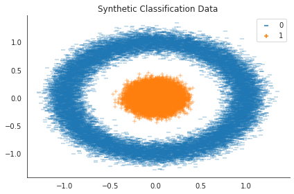
The purpose here is to turn the synthetic 2D dataset into a clear visual summary so the two classes can be inspected before any modeling begins. The x-coordinates and y-coordinates from the feature matrix are plotted against each other, and the class label is used twice: once to color the points and once to choose the marker style. That makes the two categories easy to distinguish visually, even though they occupy the same overall space. The marker choices are intentionally simple, so the main visual difference comes from the colors and the circular arrangement of the data.
After the points are drawn, the plot title is added to describe what is being shown. The axis styling is cleaned up by removing the top and right borders, which gives the figure a lighter, more presentation-friendly look. The layout is tightened so the labels and legend fit neatly without wasting space, and then the figure is saved to the results folder for later reuse.
The saved image shows exactly the kind of problem the network will need to solve: one class forms a dense inner cluster near the origin, while the other class wraps around it as a much larger outer ring. The separation is clearly not a straight line, which is why this dataset is useful for demonstrating a hidden layer. A linear classifier would struggle here, but a small neural network can learn a curved boundary that follows the shape of the circles.
Neural Network Structure
Hidden Layer Responses
The hidden layer, written as h, maps the two-dimensional input into a three-dimensional representation. For that reason, the hidden-layer weight matrix, W to the h power, has two rows and three columns, and the hidden-layer bias vector, b to the h power, contains three entries:
The hidden layer parameters are organized as a weight matrix with two input features and three hidden units, together with a bias vector for the three hidden units. The weight matrix contains the six hidden weights, arranged so that each row corresponds to one input feature and each column corresponds to one hidden neuron. The bias vector contains one bias term for each hidden unit.
The hidden layer scores, written as Z of h, are obtained by multiplying the input matrix X, which has N rows and 2 columns, by the hidden weight matrix W of h, which has 2 rows and 3 columns, and then adding the hidden bias vector b of h, which has 1 row and 3 columns:
The hidden-layer pre-activation matrix has one row per sample and three columns for the hidden units. It is obtained by multiplying the input matrix, which contains the two input features for each sample, by the hidden-layer weight matrix, and then adding the hidden-layer bias vector to every row.
The logistic sigmoid function transforms the hidden pre-activation values in Z^h through a non-linear mapping, producing the hidden-layer activations as a matrix with one row per sample and three hidden units in each row.
The hidden-layer output matrix, written as H, has one row per sample and three columns, so its shape is N by 3. It is obtained by applying the sigmoid activation to the result of multiplying the input matrix X by the hidden-layer weight matrix Wh and then adding the hidden-layer bias bh. In other words, each hidden unit receives the weighted input plus bias, and sigmoid turns that value into an activation between zero and one. The matrix can be viewed row by row as the activations for all N observations, with the first sample producing h11, h12, and h13, and the last sample producing hN1, hN2, and hN3.
def logistic(z):
    """Logistic function."""
    return 1 / (1 + np.exp(-z))
This cell defines the logistic, or sigmoid, activation function that the neural network uses in its hidden layer. It takes an input value or array called z and transforms each entry into a number between 0 and 1 by applying the standard sigmoid formula. Behind the scenes, values far below zero get pushed close to 0, values far above zero get pushed close to 1, and values near zero land around 0.5. That smooth squashing behavior is useful because it introduces nonlinearity, which is what allows the network to model the curved class boundary in the dataset instead of being limited to a straight line.
Nothing is displayed when the cell runs because it only creates a reusable function. Later cells can call this function whenever they need to turn raw weighted sums into hidden-layer activations.
def hidden_layer(input_data, weights, bias):
    """Compute hidden activations"""
    return logistic(input_data @ weights + bias)
This cell defines the function that computes the activations of the hidden layer in the neural network. It takes the incoming data, multiplies it by the hidden-layer weight matrix, adds the bias term, and then passes the result through the logistic sigmoid function. The matrix multiplication combines each input feature with each hidden unit’s weights to produce a pre-activation score for every hidden neuron, and the bias shifts those scores so the model is not forced to pass through the origin. Applying the sigmoid then squeezes those scores into values between 0 and 1, which gives the hidden layer its nonlinear behavior. That nonlinearity is what allows the network to transform the circular data into a representation that can later be separated more easily by the output layer. There is no printed result here because the cell only creates the function; it prepares a building block that the later forward pass and training steps will call whenever the hidden activations need to be computed.
Output Layer Activations
The output layer values, called Z for the output layer, form a matrix with N rows and 2 columns. They are obtained by multiplying the hidden-layer activation matrix H, which has N rows and 3 columns, by the output weight matrix W for the output layer, which has 3 rows and 2 columns, and then adding the output bias vector b for the output layer, which has 1 row and 2 columns:
The output layer forms the score matrix for all samples by multiplying the hidden layer activations, which have three columns, by the output weight matrix, which maps those three hidden units to two output classes, and then adding the output bias row to every sample.
The softmax function, written here as varsigma, converts the raw class scores into probabilities between 0 and 1 and makes sure they add up to 1 for each sample. The output is an N by 2 matrix, with one column assigned to each class label.
The model’s predicted output matrix for all N samples has N rows and 2 columns. It is produced by applying the softmax function to the output layer scores, which come from multiplying the hidden layer activations by the output weight matrix and then adding the output bias. In words, each class score is exponentiated and then divided by the sum of the exponentiated scores across all classes, so the two numbers in every row represent the predicted probabilities for the two classes. Written entry by entry, this forms a matrix whose rows contain the two predicted values for each sample, such as the first sample’s two probabilities, then the next sample’s two probabilities, and so on through sample N.
def softmax(z):
    """Softmax function"""
    return np.exp(z) / np.sum(np.exp(z), axis=1, keepdims=True)
The purpose here is to define the softmax function, which turns a set of raw output scores into probabilities. For each row of input values, the function exponentiates the scores so that larger values become more prominent, and then divides by the sum of those exponentials across the row. That normalization step is what makes the results add up to 1 for each sample, so the output can be interpreted as a probability distribution over classes. The use of axis 1 and keepdims=True means the division happens separately for each example in the batch while preserving the two-dimensional shape needed for later calculations. Since the cell only defines the function and does not call it, there is no saved output yet.
def output_layer(hidden_activations, weights, bias):
    """Compute the output y_hat"""
    return softmax(hidden_activations @ weights + bias)
This step defines the final layer of the network, the part that turns the hidden layer’s features into predicted class probabilities. It takes the activations coming out of the hidden layer, multiplies them by the output weights, adds the output bias, and then passes the result through the softmax function. Behind the scenes, that last step is what converts raw scores into values that add up to 1 for each example, so the model can interpret them as probabilities for the two classes. Since the cell only creates a function and does not call it, there is no saved output yet; it simply prepares the output-stage computation that will be used later during forward propagation and training.
Computing the Output of the Network
The forward_prop function ties the earlier steps together and computes the network’s output activations from the input data using the current weights and biases. The predict function then takes those weights, biases, and inputs and returns the binary class labels.
def forward_prop(data, hidden_weights, hidden_bias, output_weights, output_bias):
    """Neural network as function."""
    hidden_activations = hidden_layer(data, hidden_weights, hidden_bias)
    return output_layer(hidden_activations, output_weights, output_bias)
A small helper function is being defined here to package the full forward pass of the neural network into a single step. It takes the input data together with all of the learned parameters for both layers, first sends the data through the hidden layer to compute the hidden activations, and then feeds those activations into the output layer to produce the final predictions. Behind the scenes, that means it combines the linear transformation and sigmoid-style nonlinearity in the hidden layer with the final scoring and softmax conversion in the output layer. The result is a neat wrapper that represents the network as a function from raw input features to class probabilities, which makes later steps such as training, prediction, and gradient checking much simpler because they can call one routine instead of repeating the two-layer computation each time. There is no saved output because the cell only defines the function; nothing is printed or displayed yet.
def predict(data, hidden_weights, hidden_bias, output_weights, output_bias):
    """Predicts class 0 or 1"""
    y_pred_proba = forward_prop(data,
                                hidden_weights,
                                hidden_bias,
                                output_weights,
                                output_bias)
    return np.around(y_pred_proba)
The purpose here is to turn the network’s output probabilities into an actual class prediction. The model itself produces two probabilities, one for each class, after the forward pass. Rather than returning those raw probabilities, this helper runs the data through the full forward propagation step and then rounds the resulting values to the nearest whole number. For a binary classifier using softmax outputs, that rounding converts a probability vector into a one-hot-like class decision, so the larger probability is effectively turned into a 1 and the smaller one into a 0.
Behind the scenes, the function does not learn anything new or change the network parameters. It simply reuses the already defined forward pass so that prediction is consistent with how the model was trained. The saved output is empty because the cell only defines the function; nothing is computed or displayed yet. The function becomes useful later when the trained network needs to label new points or evaluate how well it separates the two classes.
Cross-Entropy Loss
The cost function, J, is based on cross-entropy loss. This loss measures how far the predicted class probabilities for each sample and class are from the true outcomes by summing those discrepancies across all samples.
The loss function, written for the entire training set, is the total of the individual sample losses. For each example, the contribution is the cross entropy between the true one hot label vector and the predicted probability vector. In other words, the overall cost is found by summing, across all samples and all classes, the true class indicator multiplied by the logarithm of the predicted probability for that class, with a negative sign applied so that better predictions produce smaller loss.
def loss(y_hat, y_true):
    """Cross-entropy"""
    return - (y_true * np.log(y_hat)).sum()
This cell defines the loss function used to measure how well the network’s predictions match the true labels. The function computes cross-entropy, which is a standard choice for classification because it strongly penalizes the model when it assigns low probability to the correct class. Inside the function, the predicted probabilities are first passed through a logarithm, then multiplied by the one-hot encoded true labels, and finally summed with a negative sign. Because the labels are one-hot, only the probability assigned to the correct class contributes for each example, so the result reflects how confidently the model supported the right answer across the dataset. There is no saved output because the cell only creates this reusable function; nothing is printed or displayed yet.
Backpropagation
Backpropagation adjusts each parameter by using the loss gradient for that parameter, and those gradients are obtained through repeated application of the chain rule.
Gradient of the Loss Function
The gradient of the loss function, J, with respect to each output-layer activation, meaning the activation produced for sample i where i runs from 1 through N, has a very simple form:
The gradient of the loss with respect to the output pre-activation for class i is the output error term, which equals the predicted probability for that class minus the true label value.
For a fuller derivation, refer to this discussion and this explanation.
def loss_gradient(y_hat, y_true):
    """output layer gradient"""
    return y_hat - y_true
The purpose here is to define the gradient of the loss with respect to the network’s output probabilities. Since the model is using softmax at the final layer together with cross-entropy loss, the derivative simplifies to a very compact form: the predicted probabilities minus the true one-hot labels. That means the error signal at the output layer is strongest for classes the model predicted too confidently and too weak for the correct class. Behind the scenes, this expression is the key starting point for backpropagation, because it turns the difference between prediction and target into the signal that gets passed backward through the rest of the network. There is no printed result from the cell itself, because it only defines a function that will be used later when gradients are computed during training or gradient checking.
Gradients for the Output Layer
Gradients for the Output Weights
To send the update information backward to the weights in the output layer, we first compute how the loss changes when the output weight matrix is adjusted:
The gradient of the loss with respect to the output weight matrix is obtained by multiplying the transpose of the hidden layer activations by the output error term. In other words, the derivative of J with respect to Wo equals the transpose of H times the difference between the predicted labels and the true labels, which is also the output layer delta.
def output_weight_gradient(H, loss_grad):
    """Gradients for the output layer weights"""
    return  H.T @ loss_grad
The purpose here is to define the gradient for the weights in the output layer, which is one of the key pieces needed for backpropagation. The function takes the hidden-layer activations and the gradient of the loss with respect to the output layer’s pre-activation values, then combines them to measure how each output weight contributed to the final error.
Behind the scenes, the hidden activations are arranged so that each row represents one training example and each column represents one hidden unit. Taking the transpose of that matrix lines up those hidden-unit values with the corresponding error signal from the output layer, and the matrix multiplication accumulates the contribution from every example in the batch. The result is a matrix of the same shape as the output weights, telling us how much each hidden-to-output connection should change to reduce the loss.
There is no saved output because the cell only defines a helper function. Nothing is computed or displayed yet; the function simply becomes available for later gradient calculations during training and gradient checking.
Updating the Output Bias
To adjust the bias terms in the output layer, we use the same chain rule approach and compute the partial derivative of the loss with respect to the bias vector:
The gradient of the loss with respect to the output bias is obtained by chaining together the sensitivity of the loss to the predicted probabilities, the effect of the softmax scores on those probabilities, and the dependence of the output scores on the bias term. After simplifying, this becomes the sum over all training examples of the output-layer error for each example. In other words, the bias gradient is the total of the output deltas across the full batch.
def output_bias_gradient(loss_grad):
    """Gradients for the output layer bias"""
    return np.sum(loss_grad, axis=0, keepdims=True)
This function computes the gradient for the bias term in the output layer. In backpropagation, each training example contributes a small error signal at the output, and the bias gradient is found by adding those signals together across all samples in the batch. Summing along the first axis collapses the per-example gradients into one row of values, which matches the shape of the output bias itself. Keeping the dimensions intact makes it easy to use the result later when updating the model parameters. Since the cell only defines the helper function and does not call it, there is no printed output yet.
Gradients for the hidden layer
The hidden-layer error signal is the gradient of the loss with respect to the hidden pre-activation values. It is obtained by chaining the gradient of the loss with respect to the hidden activations, the gradient of the output pre-activations with respect to the hidden activations, and the gradient of the hidden activations with respect to the hidden pre-activations.
def hidden_layer_gradient(H, out_weights, loss_grad):
    """Error at the hidden layer.
    H * (1-H) * (E . Wo^T)"""
    return H * (1 - H) * (loss_grad @ out_weights.T)
The purpose here is to compute the error signal for the hidden layer during backpropagation. Once the network has already measured how wrong the output layer is, that error has to be passed backward through the output weights so the hidden units can also be updated. The function takes the hidden activations, the weights connecting hidden units to the output layer, and the gradient coming from the loss at the output side.
First, the output-layer gradient is moved back through the output weights by multiplying it with the transpose of those weights. That tells us how much each hidden unit contributed to the final prediction error. Then that backward signal is adjusted by the derivative of the sigmoid activation used in the hidden layer. Since sigmoid units compress their inputs into values between 0 and 1, their sensitivity is highest in the middle and smaller near the extremes, so the factor H times one minus H captures that local slope. Multiplying these two pieces gives the full hidden-layer gradient: the part of the output error attributable to each hidden unit, scaled by how responsive that unit currently is.
Nothing is displayed when the cell runs because the function is only being defined, not called. Its effect is to make this backpropagation step available for later use when gradients are computed during training.
Gradient for the Hidden Weights
The gradient of the loss with respect to the hidden-layer weight matrix is found by taking the transpose of the input matrix and multiplying it by the hidden-layer error term.
def hidden_weight_gradient(X, hidden_layer_grad):
    """Gradient for the weight parameters at the hidden layer"""
    return X.T @ hidden_layer_grad
This helper computes the gradient for the weights that connect the input features to the hidden layer. Its job is to take the input matrix and the error signal coming back from the hidden layer, then combine them in the way backpropagation requires so we know how each input-to-hidden weight should be adjusted.
The key idea is that every hidden weight affects the loss through the hidden units, and the update for each weight depends on both the input value feeding into that weight and the gradient arriving at the hidden unit. Transposing the input matrix lines up the dimensions so each input feature can be paired with each hidden-unit gradient across all training examples. The matrix multiplication then aggregates those contributions over the whole dataset, producing the full gradient array for the hidden-layer weights.
Because the cell only defines a function, there is no saved output. Its effect is to prepare this reusable gradient calculation for later use during backpropagation and training.
Gradient of the Hidden Bias
The gradient of the loss with respect to the hidden layer bias is found by chaining together the effect of the loss on the hidden activations, then on the hidden preactivation values, and finally on the bias itself. Since the bias contributes equally to every sample, the result is the total of the hidden layer error terms across all data points.
def hidden_bias_gradient(hidden_layer_grad):
    """Gradient for the bias parameters at the output layer"""
    return np.sum(hidden_layer_grad, axis=0, keepdims=True)
This defines the gradient for the hidden-layer bias term. The idea is that once the error signal has been worked back to the hidden layer, each hidden unit needs a single bias update that reflects how much that unit contributed to the overall loss across all training examples. Because a bias affects every example in the same way, the gradient is found by summing the hidden-layer gradient across the sample dimension. Keeping the dimensions with keepdims=True preserves the row-vector shape, which makes the result easy to use later when updating the parameters. Since the cell only creates this helper function and does not call it, there is no displayed output.
Set Up the Weights
def initialize_weights():
    """Initialize hidden and output weights and biases"""

    # Initialize hidden layer parameters
    hidden_weights = np.random.randn(2, 3)
    hidden_bias = np.random.randn(1, 3)

    # Initialize output layer parameters
    output_weights = np.random.randn(3, 2)
    output_bias = np.random.randn(1, 2)
    return hidden_weights, hidden_bias, output_weights, output_bias
The purpose of this cell is to create a small random starting point for the neural network before training begins. The function bundles together all of the learnable parameters: the weights and biases for the hidden layer, and the weights and biases for the output layer. Since the network has two input features and three hidden units, the hidden weight matrix needs to connect 2 inputs to 3 hidden neurons, and the hidden bias needs one value for each hidden neuron. The output layer then takes those 3 hidden activations and maps them to 2 output classes, so its weight matrix has 3 rows and 2 columns, with a matching bias vector of length 2.
Behind the scenes, each parameter is filled with values drawn from a standard normal distribution, so the network starts with random numbers rather than zeros. That randomness is important because it gives different neurons different initial conditions, which helps the model learn useful patterns during gradient-based training. The function then returns all four arrays together so the rest of the training pipeline can use them as the initial model state.
There is no saved output here because the cell only defines the function; nothing is printed or displayed yet. The effect of running it appears later, when the function is called to initialize the network before training or gradient checking.
Calculate the gradients
def compute_gradients(X, y_true, w_h, b_h, w_o, b_o):
    """Evaluate gradients for parameter updates"""

    # Compute hidden and output layer activations
    hidden_activations = hidden_layer(X, w_h, b_h)
    y_hat = output_layer(hidden_activations, w_o, b_o)

    # Compute the output layer gradients
    loss_grad = loss_gradient(y_hat, y_true)
    out_weight_grad = output_weight_gradient(hidden_activations, loss_grad)
    out_bias_grad = output_bias_gradient(loss_grad)

    # Compute the hidden layer gradients
    hidden_layer_grad = hidden_layer_gradient(hidden_activations, w_o, loss_grad)
    hidden_weight_grad = hidden_weight_gradient(X, hidden_layer_grad)
    hidden_bias_grad = hidden_bias_gradient(hidden_layer_grad)

    return [hidden_weight_grad, hidden_bias_grad, out_weight_grad, out_bias_grad]
The purpose of this cell is to bundle the whole backpropagation step into one helper so the network can later be trained repeatedly without re-deriving anything each time. It takes the input data, the true labels, and the current weights and biases, then runs a full forward pass to see what the network is predicting at the moment. First it sends the inputs through the hidden layer to get the hidden activations, and then it passes those activations through the output layer to produce the predicted probabilities.
Once the predictions are available, the cell moves backward through the network to measure how each parameter should change to reduce the loss. It starts at the output layer by computing the loss gradient, which captures the difference between the predicted probabilities and the true one-hot labels. From that signal it computes the gradient for the output weights and the output bias. Then it propagates the error back into the hidden layer, where the gradient is adjusted by the output weights and the activation function’s derivative. Using that hidden-layer error signal, it calculates the gradients for the hidden weights and hidden bias.
The final return value is an ordered collection of the four gradients: hidden weights, hidden bias, output weights, and output bias. That order matters because it matches the way the parameters are usually updated later in training. There is no saved output because the cell only defines a function; nothing is printed or displayed yet.
Verify the Gradients
Backpropagation involves many parameter inputs, so it is easy to introduce errors. One practical way to verify that the implementation is correct is to compare the output change caused by a tiny perturbation in the parameters with the output change predicted by the gradient that was calculated. For a fuller explanation, see here.
# change individual parameters by +/- eps
eps = 1e-4

# initialize weights and biases
params = initialize_weights()

# Get all parameter gradients
grad_params = compute_gradients(X, Y, *params)

# Check each parameter matrix
for i, param in enumerate(params):
    # Check each matrix entry
    rows, cols = param.shape
    for row in range(rows):
        for col in range(cols):
            # change current entry by +/- eps
            params_low = deepcopy(params)
            params_low[i][row, col] -= eps

            params_high = deepcopy(params)
            params_high[i][row, col] += eps

            # Compute the numerical gradient
            loss_high = loss(forward_prop(X, *params_high), Y)
            loss_low = loss(forward_prop(X, *params_low), Y)
            numerical_gradient = (loss_high - loss_low) / (2 * eps)

            backprop_gradient = grad_params[i][row, col]

            # Raise error if numerical and backprop gradient differ
            assert np.allclose(numerical_gradient, backprop_gradient), ValueError(
                    f'Numerical gradient of {numerical_gradient:.6f} not close to '
                    f'backprop gradient of {backprop_gradient:.6f}!')

print('No gradient errors found')
No gradient errors foundThe purpose of this cell is to verify that the backpropagation formulas are correct before any training begins. It starts by choosing a very small change size, called epsilon, which will be used to test how sensitive the loss is to tiny shifts in each parameter. Then it creates a fresh set of random weights and biases, and computes the gradients for those parameters using the backpropagation implementation.
From there, the cell checks every single entry in every parameter matrix one by one. For each value, it makes two nearly identical copies of the model parameters: one slightly smaller and one slightly larger at just that one position. It then runs the network forward with each modified version, calculates the loss in both cases, and uses the difference between those two losses to estimate the numerical gradient. This finite-difference estimate is a standard way to approximate the true derivative directly from the loss surface.
That numerical estimate is then compared against the gradient produced by backpropagation for the same parameter entry. If the two values are not close enough, the assertion triggers an error and reports exactly which gradient disagreed. This makes the cell a careful consistency check: if the mathematical derivation or its NumPy implementation were wrong, the mismatch would show up here before training ever starts.
The saved output, “No gradient errors found,” means every numerical gradient matched the corresponding backpropagation gradient within the allowed tolerance. In other words, the model’s gradient calculations are behaving as expected, and the training code can rely on them.
Train the Network
def update_momentum(X, y_true, param_list,
                    Ms, momentum_term,
                    learning_rate):
    """Update the momentum matrices."""
    # param_list = [hidden_weight, hidden_bias, out_weight, out_bias]
    # gradients = [hidden_weight_grad, hidden_bias_grad,
    #               out_weight_grad, out_bias_grad]
    gradients = compute_gradients(X, y_true, *param_list)
    return [momentum_term * momentum - learning_rate * grads
            for momentum, grads in zip(Ms, gradients)]
The purpose here is to turn the current model parameters and the training data into a new set of momentum updates. The function first calls the gradient computation routine, which runs a forward pass through the network and then backpropagates the error to get the derivatives for each parameter group. Those gradients are collected in the same order as the parameters themselves, so each weight matrix and bias vector has a matching gradient.
After that, the function combines the new gradients with the previous momentum values. For each parameter, it keeps part of the old momentum, scaled by the momentum factor, and then subtracts a step in the direction of the gradient, scaled by the learning rate. The result is not the updated parameters directly, but the velocity terms that will be used to move the parameters in the next step. That is how momentum works behind the scenes: it smooths out the updates by letting the optimizer keep some memory of earlier gradients, which can help the training process move more steadily through the loss landscape.
There is no saved output because the cell only defines this helper function. Nothing is printed or displayed yet; the function simply becomes available for later training steps, where it will be used together with the parameter update function to actually adjust the network during optimization.
def update_params(param_list, Ms):
    """Update the parameters."""
    # param_list = [Wh, bh, Wo, bo]
    # Ms = [MWh, Mbh, MWo, Mbo]
    return [P + M for P, M in zip(param_list, Ms)]
The purpose here is to apply the momentum-adjusted changes to the model’s parameters after the gradients have already been turned into update steps. The function takes two parallel lists: one containing the current parameters of the network, and the other containing the momentum terms that were computed from the gradients. It then pairs each parameter with its matching update using zip and adds them together. Because the momentum terms already encode the direction and size of the step to take, adding them to the parameters produces the next version of the weights and biases. Nothing is printed or displayed when the cell runs, since the function definition only prepares this reusable update rule for later training steps.
def train_network(iterations=1000, lr=.01, mf=.1):
    # Initialize weights and biases
    param_list = list(initialize_weights())

    # Momentum Matrices = [MWh, Mbh, MWo, Mbo]
    Ms = [np.zeros_like(M) for M in param_list]

    train_loss = [loss(forward_prop(X, *param_list), Y)]
    for i in range(iterations):
        if i % 1000 == 0: print(f'{i:,d}', end=' ', flush=True)
        # Update the moments and the parameters
        Ms = update_momentum(X, Y, param_list, Ms, mf, lr)

        param_list = update_params(param_list, Ms)
        train_loss.append(loss(forward_prop(X, *param_list), Y))

    return param_list, train_loss
The purpose here is to package the whole training process into a single reusable function. It starts by creating the network’s initial parameters, which means the hidden-layer weights and biases and the output-layer weights and biases are all sampled once at random. Those values are collected into one list so they can be passed around together during training.
Right after that, a matching set of momentum arrays is created. These start out as zeros and have the same shapes as the parameters they correspond to. Behind the scenes, these arrays act like memory for the optimizer: instead of updating the weights only from the current gradient, the training step also keeps part of the previous update, which helps smooth the optimization path and can make learning less jittery.
Before any updates happen, the function measures the current loss on the full training set and stores it as the first entry in the loss history. Then it enters the training loop. At each iteration, it prints the iteration number every 1000 steps so progress can be monitored without flooding the output. The actual learning happens in two stages: first the momentum values are updated using the current gradients, learning rate, and momentum factor; then those momentum values are applied to adjust the parameters themselves. After each update, the function computes the new loss again and appends it to the history list, so the training curve can be inspected later.
When the loop finishes, the function returns both the final learned parameters and the full sequence of loss values. There is no saved output shown for this cell because the cell only defines the training function; it does not run training yet.
If you have a chance, try the different parameter settings and compare how they perform.
# n_iterations = 20000
# results = {}
# for learning_rate in [.01, .02, .05, .1, .25]:
#     for momentum_factor in [0, .01, .05, .1, .5]:
#         print(learning_rate, momentum_factor)
#         trained_params, train_loss = train_network(iterations=n_iterations, lr=learning_rate, mf=momentum_factor)
#         results[(learning_rate, momentum_factor)] = train_loss[::1000]
The purpose of this cell is to set up a small experiment for comparing different training settings. It is essentially preparing a sweep over several learning rates and momentum values so the model can be trained multiple times under different optimization choices. The first line fixes the number of training iterations for each run, and the next line creates an empty dictionary to store the results from each combination.
The nested loops then move through each learning rate and each momentum factor in turn. For every pair, the cell prints the values so you can see which setting is being tested, then calls the training routine with those hyperparameters. That training routine returns the learned parameters and the loss history, and only every thousandth loss value is kept so the results are easier to compare later. Each loss trace is saved in the dictionary using the learning rate and momentum pair as the key, which makes it simple to look up or plot the behavior of any particular run afterward.
There is no saved output because the experiment code is commented out, so nothing actually runs here. As written, the cell serves as a ready-made template for a grid search over optimization settings, but it does not execute any training until those comment markers are removed.
trained_params, train_loss = train_network(iterations=n_iterations,
                                           lr=learning_rate,
                                           mf=momentum_factor)
0 1,000 2,000 3,000 4,000 5,000 6,000 7,000 8,000 9,000 10,000 11,000 12,000 13,000 14,000 15,000 16,000 17,000 18,000 19,000 20,000 21,000 22,000 23,000 24,000 25,000 26,000 27,000 28,000 29,000 30,000 31,000 32,000 33,000 34,000 35,000 36,000 37,000 38,000 39,000 40,000 41,000 42,000 43,000 44,000 45,000 46,000 47,000 48,000 49,000The cell starts the actual training run for the neural network by calling the training routine with the chosen number of iterations, learning rate, and momentum factor. Inside that routine, the model begins from randomly initialized weights and biases, then repeatedly cycles through forward propagation, loss calculation, gradient computation, and parameter updates. As training progresses, the two sets of parameters are adjusted together so the network gradually improves its ability to separate the two classes in the circle dataset.
The saved output is the progress display from that long optimization loop. The numbers appear at regular intervals because the training function is set up to print updates every 1,000 iterations, giving a simple checkpoint view of how far the run has advanced. Since the training is being done for 50,000 iterations, the output counts upward from 0 through 49,000, showing that the loop is steadily moving through the full training schedule. There is no final loss value printed here, so the visible result of the cell is mainly confirmation that the model is being trained as intended and that the optimization process is running over the full range of iterations.
hidden_weights, hidden_bias, output_weights, output_bias = trained_paramsThe cell simply takes the four learned parameter arrays produced by training and unpacks them into separate names for the hidden layer weights, hidden layer bias, output layer weights, and output layer bias. At this point, the network has already been trained, so these values represent the final fitted model rather than random starting values. Separating them back out makes it easier to use the trained network for later steps such as generating predictions, drawing the decision boundary, or inspecting what each layer has learned. Since the assignment only stores existing values into new variables, nothing is printed or displayed when the cell runs.
Visualize the Training Loss
This figure shows how the training loss changes across 50 thousand iterations when the model is trained on 50 thousand samples using a momentum value of 0.5 and a learning rate of 1e-4.
The curve indicates that the loss does not begin to fall until after roughly 5 thousand iterations, but once it starts improving, the drop becomes very steep. Since stochastic gradient descent was not used here, convergence would probably have been much faster with that approach.
ax = pd.Series(train_loss).plot(figsize=(12, 3), title='Loss per Iteration', xlim=(0, n_iterations), logy=True)
ax.set_xlabel('Iteration')
ax.set_ylabel('$\\log \\xi$', fontsize=12)
sns.despine()
plt.tight_layout()
plt.savefig(results_path / 'ffnn_loss', dpi=300)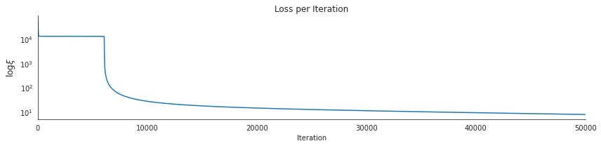
The purpose of this cell is to turn the recorded training losses into a clear visual summary of how learning progressed over time. It starts by wrapping the list of loss values in a pandas Series so it can be plotted directly, then draws that series as a line chart with a wide, short figure size that makes long training runs easy to read. The title and axis limits are set so the plot spans the full training range from the first to the last iteration, and the y-axis is displayed on a logarithmic scale. That log scale is important because the loss changes by large factors during training, and plotting it this way makes both the early sharp drop and the later slower improvements visible on the same chart.
Next, the axes are labeled to show that the horizontal direction is iteration number and the vertical direction is the logarithm of the loss. The call to remove the top and right borders makes the figure cleaner and easier to interpret, and the layout adjustment helps prevent labels from being cut off. Finally, the plot is saved to the results folder so it can be reused outside the notebook.
The saved figure reflects exactly this sequence of operations. It shows a very high loss at the beginning, followed by a steep decline in the early iterations and then a much gentler downward slope as training continues. That shape is what you would expect from gradient-based learning: the model starts out poorly fitted, quickly finds a much better region of parameter space, and then makes smaller refinements as it approaches a solution. The fact that the curve keeps trending downward rather than flattening immediately suggests the network is still improving throughout training, even if the gains become more gradual over time.
Decision Boundary
The plots below illustrate the mapping learned by the neural network when a three unit hidden layer is applied to two dimensional data containing two classes that cannot be separated by a straight line, as shown in the left panel. The decision boundary correctly classifies nearly all points, and additional training would likely reduce the remaining mistakes.
The middle plot displays the feature representation produced by the hidden layer. During training, the network adjusts the hidden weights so that the original two dimensional inputs are transformed into a three dimensional space where the two classes can be separated with a linear boundary.
The final plot shows how the output layer carries out that separation by using a threshold of 0.5 on the output value.
n_vals = 200
x1 = np.linspace(-1.5, 1.5, num=n_vals)
x2 = np.linspace(-1.5, 1.5, num=n_vals)
xx, yy = np.meshgrid(x1, x2)  # create the grid

# Initialize and fill the feature space
feature_space = np.zeros((n_vals, n_vals))
for i in range(n_vals):
    for j in range(n_vals):
        X_ = np.asarray([xx[i, j], yy[i, j]])
        feature_space[i, j] = np.argmax(predict(X_, *trained_params))
The purpose here is to evaluate the trained neural network across a dense grid of points in the input plane so the model’s behavior can later be visualized as a surface or decision map. It starts by choosing 200 evenly spaced values along each axis from about minus 1.5 to 1.5, which creates a square region covering the area where the circular data lives. Those two one-dimensional arrays are then combined into a full grid of coordinate pairs, so every position in that square has a matching x and y location.
After the grid is built, an empty two-dimensional array is created to store the model’s predicted class at each grid point. The nested loops then walk through every coordinate in the grid one by one. For each position, the pair of coordinates is assembled into a tiny input sample shaped the way the network expects, and the trained model is asked to predict class probabilities for that point. The prediction is converted into a class label by taking the index of the larger output probability, and that label is written into the matching spot in the feature-space array.
Nothing is displayed yet, which is why there is no saved output from this cell. Its job is preparatory: it builds the full grid of predicted classes that later plotting cells can use to draw the learned decision boundary or a colored surface. The resulting array captures how the network partitions the plane into class regions, point by point, based on everything it learned during training.
# Create a color map to show the classification colors of each grid point
cmap = ListedColormap([sns.xkcd_rgb["pale red"],
                       sns.xkcd_rgb["denim blue"]])

# Plot the classification plane with decision boundary and input samples
plt.contourf(xx, yy, feature_space, cmap=cmap, alpha=.25)

# Plot both classes on the x1, x2 plane
data = pd.DataFrame(X, columns=['$x_1$', '$x_2$']).assign(Class=pd.Series(y).map({0:'negative', 1:'positive'}))
sns.scatterplot(x='$x_1$', y='$x_2$', hue='Class', data=data, style=y, markers=['_', '+'], legend=False)
plt.title('Decision Boundary')
sns.despine()
plt.tight_layout()
plt.savefig(results_path / 'boundary', dpi=300);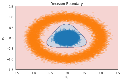
The purpose here is to visualize the model’s decision boundary directly in the original two-dimensional input space and compare it against the training samples. To do that, a two-color colormap is created first so the background can show the two predicted classes with soft, readable shading. The classification scores that were already computed on a dense grid of points are then drawn as a filled contour plot, which paints each region of the plane according to the class the network assigns there. Because the contour is semi-transparent, it acts like a backdrop rather than hiding everything else.
After the background is in place, the original data points are assembled into a small table with the two input coordinates and a human-readable class label. Those samples are plotted on top of the decision regions with different colors and markers, so you can see where the real examples fall relative to the boundary the network learned. The title is added for clarity, the plot styling is cleaned up by removing extra spines, and the layout is tightened so the figure is neatly arranged. Finally, the image is saved to the results folder for later use.
The saved figure shows exactly what this sequence is meant to reveal. The pale background areas represent the model’s predicted class regions, while the orange and blue points show the two circular classes in the dataset. The boundary curves around the inner cluster rather than drawing a straight line, which is the key sign that the neural network has learned a nonlinear separation. The inner blue group is surrounded by the outer orange ring, so a linear classifier would struggle here, but the curved boundary indicates the network has captured the circular structure of the problem.
Hidden-Layer Projection
n_vals = 25
x1 = np.linspace(-1.5, 1.5, num=n_vals)
x2 = np.linspace(-1.5, 1.5, num=n_vals)
xx, yy = np.meshgrid(x1, x2)  # create the grid
X_ = np.array([xx.ravel(), yy.ravel()]).T
The purpose here is to build a regular grid of 2D points that can later be fed through the trained network for visualization. It starts by choosing 25 evenly spaced values between -1.5 and 1.5 for the first coordinate and then does the same for the second coordinate. Those two one-dimensional ranges are combined into a meshgrid, which creates every possible pairing of x1 and x2 across the square region. From there, the grid is flattened and rearranged into a two-column array where each row represents one point in the plane.
Behind the scenes, this turns a neat square lattice into a format that matches the network’s expected input shape. Instead of thinking about the points as a 25 by 25 grid, the data is converted into a list of 625 coordinate pairs. That makes it easy to pass all the locations through the model at once when plotting a decision boundary or a probability surface later on. Since the cell is only preparing coordinates and not displaying anything yet, there is no saved output.
fig = plt.figure(figsize=(6, 4))
with sns.axes_style("whitegrid"):
    ax = Axes3D(fig)

ax.plot(*hidden_layer(X[y == 0], hidden_weights, hidden_bias).T,
        '_', label='negative class', alpha=0.75)
ax.plot(*hidden_layer(X[y == 1], hidden_weights, hidden_bias).T,
        '+', label='positive class', alpha=0.75)

ax.set_xlabel('$h_1$', fontsize=12)
ax.set_ylabel('$h_2$', fontsize=12)
ax.set_zlabel('$h_3$', fontsize=12)
ax.view_init(elev=30, azim=-20)
# plt.legend(loc='best')
plt.title('Projection of X onto the hidden layer H')
sns.despine()
plt.tight_layout()
plt.savefig(results_path / 'projection3d', dpi=300)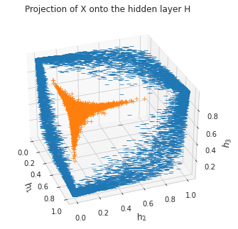
The cell creates a 3D visualization of how the original two-dimensional data looks after it has been transformed by the network’s hidden layer. Instead of plotting the raw input points, it first feeds the samples through the hidden-layer function, which turns each 2D example into a point in a three-dimensional hidden-feature space. That matters because the network is trying to make a difficult nonlinear problem easier to separate by moving it into a representation where the classes have a simpler structure.
The plot is set up with a white grid style and a 3D axis, so the result has depth and can show all three hidden units at once. The points for the negative class and positive class are handled separately, which is why the figure uses different markers for each group. Each class is plotted using the three hidden activations as its x, y, and z coordinates, so the axes are labeled as h1, h2, and h3. What appears in the saved image is the hidden-layer embedding of the training set: the two classes no longer just sit in the original circular arrangement, but instead form two distinct clouds with a noticeable geometric structure. That shape reflects how the sigmoid hidden units respond differently to the two classes and shows that the network has learned a nonlinear projection that helps separate them.
The viewpoint is then adjusted with a chosen elevation and azimuth so the 3D arrangement is easier to read. The title is added to make clear that the figure is showing the projection of X onto the hidden layer H. Finally, the plot is tightened up, cleaned with despine, and saved to the results folder. The saved output displays that final 3D scatter plot, with the two classes spread through hidden space in a way that suggests the network has extracted useful features for classification.
Plot of the Network Output Surface
zz = forward_prop(X_, hidden_weights, hidden_bias, output_weights, output_bias)[:, 1].reshape(25, -1)
zz.shape
(25, 25)The purpose here is to take the model’s output probabilities for a grid of input points and reshape them into a form that is easy to visualize as a surface or heatmap. The forward propagation step produces, for each point in X, a pair of class probabilities from the trained network. By selecting the second probability column, the cell focuses on the model’s estimated likelihood for one of the two classes. That one-dimensional list of probabilities is then reshaped into a 25 by 25 array, which matches the grid structure of the input points. Behind the scenes, this works because X was built from a regular mesh of 625 points laid out as 25 rows and 25 columns in the input space, so the corresponding predictions can be folded back into the same layout.
The saved output confirms that the reshape worked as intended. The reported shape of (25, 25) means the probability values now sit in a matrix that mirrors the original grid, making it suitable for plotting a smooth decision surface or contour view.
fig = plt.figure()
with sns.axes_style("whitegrid"):
    ax = fig.gca(projection='3d')
ax.plot_surface(xx, yy, zz, alpha=.25)
ax.set_title('Learned Function')
ax.set_xlabel('$x_1$', fontsize=12)
ax.set_ylabel('$x_2$', fontsize=12)
ax.set_zlabel('$y$', fontsize=12)
ax.view_init(elev=45, azim=-20)
sns.despine()
fig.tight_layout()
fig.savefig(results_path / 'surface', dpi=300);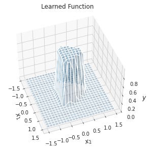
The purpose of this cell is to turn the model’s predicted values over a two-dimensional grid into a 3D surface plot, so you can see the learned function as a smooth landscape instead of just as class labels. It begins by creating a fresh figure and then switches the axes styling to a white grid, which gives the plot a clean scientific look and makes the 3D mesh easier to read. After that, it creates a 3D axis on the figure, which is what allows the next plotting step to draw a surface rather than a flat line or scatter plot.
The surface itself is drawn from the three arrays already prepared earlier: xx and yy represent the grid of input coordinates across the x1 and x2 directions, and zz holds the model’s output value at each of those grid points. Plotting those three arrays together produces a continuous sheet that shows how the network responds across the input space. The transparency is set fairly low, so the surface doesn’t overpower the figure and the grid structure remains visible.
Once the surface is drawn, the cell labels the plot with a title and axis names so the meaning of each dimension is clear. The x and y axes correspond to the two input features, while the vertical axis shows the model output. The view angle is then adjusted to a particular elevation and rotation so the shape of the surface is easier to interpret from an informative perspective. That choice of angle helps reveal the steep central region and the flatter surrounding areas.
The call to despine removes some of the extra axis framing for a cleaner presentation, and tight layout makes sure the labels and plot elements fit neatly within the figure boundaries. Finally, the figure is saved to disk at the end, so the rendered visualization is preserved for later use.
The saved output shows a tall, narrow rise in the middle of an otherwise low surface, which reflects how the trained network has concentrated high output values in the region associated with one class and low values elsewhere. The shape is not a simple plane because the model has learned a nonlinear decision function. The stepped, grid-like appearance comes from evaluating the network on a discrete mesh of input points and then connecting those values into a surface, so the plot visualizes both the geometry of the input space and the smoothness of the learned mapping.
Summary
In short, this notebook has shown that a small network with one hidden layer of three units and 17 total parameters can learn a nonlinear classification task when trained with backpropagation and gradient descent with momentum.
Next, we will revisit several important design decisions that help when building and training larger models. After that, we will move on to widely used deep learning libraries, which supply many of these pieces directly and handle automatic differentiation so that gradient computation and backpropagation become much easier to implement.
Notebook 2 of 5: 02_how_to_use_tensorflow
Source file: `02_how_to_use_tensorflow_processed.ipynb`
Getting started with TensorFlow 2
Keras was created as a high-level, or meta, API to make it easier and faster to experiment with the design and training of deep neural networks using backends such as TensorFlow, Theano, or CNTK. In 2017, it became part of TensorFlow, and with the TensorFlow 2.0 release it is intended to serve as the main interface. You can also mix TensorFlow and Keras code in the same project, which lets you use Keras for its simpler abstractions while still adding custom TensorFlow graph operations when needed.
Please refer to the setup steps in Installation Guide.md located in the project root.
Imports and configuration
import warnings
warnings.filterwarnings('ignore')
The purpose here is to quiet down warning messages so the rest of the notebook runs more cleanly. The warnings module is imported first, which gives access to Python’s built-in warning system, and then the warning filter is set to ignore warnings. After that, any warnings that would normally be printed to the output area are suppressed, so the notebook stays focused on the results that matter rather than on routine notices or deprecation messages. Since this cell only changes how warnings are displayed and does not produce a result itself, there is no saved output.
%matplotlib inline

from pathlib import Path
from copy import deepcopy
import numpy as np
import pandas as pd

import sklearn
from sklearn.datasets import make_circles # To generate the dataset

import tensorflow as tf
from tensorflow.keras.models import Sequential
from tensorflow.keras.layers import Dense, Activation
from tensorflow.keras import optimizers
from tensorflow.keras.callbacks import TensorBoard

import matplotlib
import matplotlib.pyplot as plt
from matplotlib.colors import ListedColormap
from mpl_toolkits.mplot3d import Axes3D  # 3D plots

import seaborn as sns
The purpose here is to gather everything needed for the rest of the notebook and to prepare the notebook interface for plotting. The line that enables inline plotting tells Jupyter to draw figures directly beneath the cell instead of opening separate windows, which is why later charts can appear right inside the notebook.
After that, the cell imports a set of standard tools that will support data handling, model building, and visualization. The file and copy utilities are brought in for working with paths and making independent copies of objects when needed. NumPy and pandas provide general-purpose numerical and tabular data support, while scikit-learn supplies the synthetic circles dataset generator that will create the toy classification problem. TensorFlow and several Keras components are imported next because they will be used to define, train, and monitor a neural network. The model-building pieces include a simple sequential model container, dense layers, activation functions, and an optimizer module, along with TensorBoard so training results can be logged and explored later.
The plotting libraries come in last. Matplotlib provides the basic plotting machinery, including support for customizing colors and drawing 3D figures if needed, while Seaborn will be used for cleaner statistical plots. Nothing is printed yet, so there is no saved output from this cell; its job is simply to load the tools that the following cells rely on.
# plotting style
sns.set_style('white')
# for reproducibility
np.random.seed(seed=42)
The purpose here is to set up a consistent visual style for any plots that come later and to make the random parts of the notebook repeatable. The plotting style is switched to a clean white background, which gives charts a lighter, simpler appearance and helps the data stand out more clearly against the axes. After that, the random number generator for NumPy is seeded with a fixed value, so any future random operations that rely on NumPy will produce the same results each time the notebook is run. There is no saved output because nothing is being displayed or printed yet; the cell is quietly preparing the environment for the next steps, especially for plots and synthetic data generation that need to behave consistently.
gpu_devices = tf.config.experimental.list_physical_devices('GPU')
if gpu_devices:
    print('Using GPU')
    tf.config.experimental.set_memory_growth(gpu_devices[0], True)
else:
    print('Using CPU')
Using CPUThe cell checks what kind of hardware TensorFlow can see before any heavier computation starts. It asks TensorFlow for the available physical devices of type GPU, and then uses that result to decide how the session should behave. If at least one GPU is found, the message would announce that the GPU is being used, and TensorFlow would be told to grow GPU memory gradually instead of taking all of it at once. That memory-growth setting is a practical safeguard, especially in shared or limited environments, because it helps prevent TensorFlow from reserving more GPU memory than it immediately needs.
The saved output shows that no GPU was detected, so the fallback path was taken instead. That is why the cell prints “Using CPU.” In other words, TensorFlow looked for a GPU, found an empty list, and the notebook continued with CPU-based execution. The output is short because the cell’s only visible effect in that case is the single status message confirming which device will be used.
results_path = Path('results')
if not results_path.exists():
    results_path.mkdir()
The purpose here is to make sure there is a place on disk where the notebook can store anything it produces later, especially training logs and other saved results. A Path object is created for a folder named results, and then the notebook checks whether that folder already exists. If it does not, the folder is created. Behind the scenes, this is a simple safety step: it avoids errors later when other cells try to write files into that location. Since there is no saved output, nothing is printed to the screen; the effect is just a quiet setup step that prepares the working directory for the rest of the notebook.
Data Input
Create synthetic data
The target variable y contains two classes created from circular patterns, and they cannot be separated with a straight line because class 0 encircles class 1.
# dataset params
N = 50000
factor = 0.1
noise = 0.1
This cell sets the basic settings for the synthetic dataset that will be generated next. The value for N controls how many examples the dataset will contain, so choosing 50,000 creates a fairly large sample for training and testing the neural network. The factor value is used later to control how tightly the two circular classes are nested inside one another, so a small value like 0.1 keeps the inner circle much smaller than the outer one. The noise value adds randomness to the points, which makes the problem less perfectly clean and more realistic, since the samples will not lie exactly on ideal circles.
There is no output here because nothing is being displayed yet. The cell simply prepares a few parameters that other cells will use when the data is generated, so its effect is to establish the shape and difficulty of the classification problem rather than to produce a visible result immediately.
# generate data
X, y = make_circles(
    n_samples=N,
    shuffle=True,
    factor=factor,
    noise=noise)
This step creates the synthetic dataset that the rest of the notebook uses for classification. The goal is to generate a set of two-dimensional points arranged in a pattern that is not easy to separate with a straight line, so the neural network has something meaningful to learn. The data comes from a circles generator, which produces two concentric ring-shaped classes. The number of points is set by the sample count defined earlier, and the points are shuffled so the class order is mixed rather than grouped together. The factor controls how far apart the two rings are, while the noise adds randomness so the points are not perfectly regular.
The result is stored in two variables: X for the input coordinates and y for the class labels. Since the cell only prepares the dataset and does not print or plot anything, there is no saved output. The effect of the cell is still important, though, because it defines the training data that later cells will reshape, visualize, and feed into the neural network.
# define outcome matrix
Y = np.zeros((N, 2))
for c in [0, 1]:
    Y[y == c, c] = 1
The goal here is to turn the original class labels into a format that the neural network can work with more easily. A new array is created with one row for each sample and two columns, matching the two possible classes in the problem. At first, every entry is set to zero, so the matrix starts as all zeros.
The loop then goes through the two class values, 0 and 1. For each class, it finds all samples whose label matches that class and sets the corresponding column in the new matrix to 1. That means samples from class 0 get a 1 in the first column, and samples from class 1 get a 1 in the second column. The result is a one-hot encoded target matrix, where each row contains a simple binary indicator of the class.
There is no saved output because this cell only prepares the target data in memory. Nothing is printed or displayed, but the variable Y is now ready to be used as the model’s training target.
f'Shape of: X: {X.shape} | Y: {Y.shape} | y: {y.shape}''Shape of: X: (50000, 2) | Y: (50000, 2) | y: (50000,)'The purpose here is to quickly check that the generated dataset has the shapes the model expects before moving on to training. The expression builds a formatted text message from the shape information stored in the three variables: X for the input features, Y for the one-hot encoded targets, and y for the original class labels. Behind the scenes, the shape attribute reports the dimensions of each array, so you can confirm not just the number of samples but also how many values each sample contains.
The saved output shows that X has shape (50000, 2), which means there are 50,000 data points and each one has two input coordinates. Y also has shape (50000, 2), which matches the one-hot encoding of a binary target, giving two output columns per sample. The original labels y have shape (50000,), which is a one-dimensional array with one class label per sample. That combination confirms the data was prepared consistently: two input features, two encoded target values, and one original label for each example.
Show the data visually
sns.scatterplot(x=X[:, 0],
                y=X[:, 1],
                hue=y,
               style=y,
               markers=['_', '+']);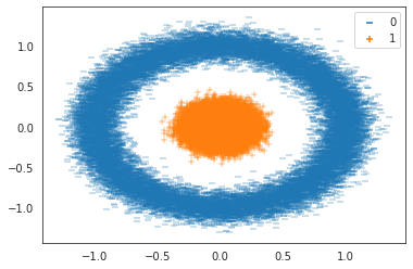
A scatter plot is being created to show the two classes in the dataset directly in the plane defined by the two input features. The horizontal positions come from the first column of X, and the vertical positions come from the second column, so every sample is placed according to its 2D coordinates. Coloring the points by y separates the two classes visually, and using style with the same labels gives each class a distinct marker shape as well. The custom markers help reinforce that there are two different groups, even before looking at the colors.
The saved figure makes the structure of the data very clear: one class forms a ring around the other. That circular pattern is exactly why the problem is interesting for a neural network, because a straight line would not be able to separate the classes well. The outer ring is shown in blue with one marker style, while the inner cluster appears in orange with another, so the plot immediately shows a nonlinearly separable dataset.
Construct the Keras Model
Keras offers two main ways to define models: the straightforward Sequential API and the more adaptable Functional API. Here, we will start with Sequential, and later chapters will use the Functional API for more involved models.
Building a model only requires creating a Sequential instance and passing in a list of layers in the order they should be applied, along with each layer’s settings such as the number of units, the activation function, and the layer name.
Set Up the Model Structure
model = Sequential([
    Dense(units=3, input_shape=(2,), name='hidden'),
    Activation('sigmoid', name='logistic'),
    Dense(2, name='output'),
    Activation('softmax', name='softmax'),
])
The model is being assembled as a small feedforward network for a problem with two input features and two output classes. It starts with a dense hidden layer containing three neurons, and the input shape is set to two because each example in the dataset has exactly two coordinates. Giving the hidden layer a name makes it easier to inspect later, especially when looking at weights or layer summaries.
After that hidden layer, a sigmoid activation is added. This introduces nonlinearity, which is important because the classes are arranged in a curved pattern and cannot be separated well by a straight line alone. The next dense layer produces two raw output values, one for each class. Those values are then passed through a softmax activation, which turns them into probabilities that add up to one. That makes the network’s final prediction easy to interpret as a choice between the two classes.
No output is shown for the cell because it only defines the architecture. The actual effects appear later when the model is compiled, trained, and summarized, at which point Keras uses this layer stack to learn from the data.
The first hidden layer must be told how many features appear in the input matrix it gets from the input layer, and that is provided through the input_shape argument. In this example, there are only two features. The number of rows processed at training time is not fixed in the model definition; instead, Keras determines it from the batch_size value that will be supplied to the fit method later.
For every layer after the first one, Keras uses the units setting from the preceding layer to determine the size of the incoming data.
Keras includes a wide selection of ready-made components, such as recurrent and convolutional layers, several regularization choices, many loss functions and optimizers, and tools for preprocessing, visualization, and logging. For more detail, the project documentation on GitHub is a useful reference. It can also be extended when the built-in options are not enough.
Calling the model’s summary method gives a compact overview of the network structure. This includes the types of layers, their output shapes, and the total number of parameters:
model.summary()Model: "sequential"
_________________________________________________________________
Layer (type) Output Shape Param #
=================================================================
hidden (Dense) (None, 3) 9
_________________________________________________________________
logistic (Activation) (None, 3) 0
_________________________________________________________________
output (Dense) (None, 2) 8
_________________________________________________________________
softmax (Activation) (None, 2) 0
=================================================================
Total params: 17
Trainable params: 17
Non-trainable params: 0
_________________________________________________________________The purpose here is to inspect the neural network that has just been built and verify its structure before moving on. Printing the model summary gives a compact architectural report, which is especially useful in Keras because it shows how the layers are connected, what shape of data flows through them, and how many parameters the network will learn.
The output starts by naming the model as “sequential,” which tells you the layers are stacked one after another in a simple linear order. The first learned layer is the hidden dense layer, and its output shape is shown as an unspecified batch size followed by 3 units. The “None” in that shape stands for the number of samples in a batch, which can vary from one training step to another. The parameter count of 9 comes from the fact that each of the 3 neurons receives 2 input values plus its own bias term, so there are 3 times 3 trainable values in total.
Right after that comes the activation layer labeled “logistic.” It keeps the same output shape because activation layers do not change the size of the data; they only apply a nonlinear transformation to the numbers already produced by the previous layer. Since activation layers have no weights of their own, their parameter count is 0.
The next dense layer is the output layer, which produces 2 values per sample. That matches the binary classification setup where the model predicts probabilities for two classes. Its parameter count of 8 follows the same pattern as before: each of the 2 output neurons receives 3 incoming values from the hidden layer, plus a bias term for each neuron. Finally, the softmax activation turns those two raw output scores into class probabilities that add up to 1, which is why its output shape stays at 2 and it also has no parameters.
At the bottom, the summary totals everything up: 17 trainable parameters and no non-trainable ones. That confirms the entire network is very small and fully learnable, which makes sense for a simple toy classification problem.
Compile the Model
The next step is to compile the Sequential model so its training behavior is fully defined. At this point, we specify the optimizer, the loss function, and one or more metrics that will be tracked while the model learns:
model.compile(optimizer='rmsprop',
              loss='binary_crossentropy',
              metrics=['accuracy'])
Before training can begin, the model needs to be configured with the rules it will use to learn from data. This step tells Keras three important things: how the network should update its weights, how to measure how wrong its predictions are, and which performance score to keep track of while training. The optimizer here is RMSprop, which is a gradient-based method that adjusts the weights in small, adaptive steps so the network can gradually improve. The loss function is binary crossentropy, which is a common choice when the task is binary classification and the model is predicting class probabilities. The accuracy metric is included so Keras can report, at each epoch, how often the model’s predictions match the true labels.
Behind the scenes, this command does not train the model yet. Instead, it prepares the model’s internal training machinery so that the next call to fit knows exactly how to compute errors, how to update parameters, and what summaries to display. Since there is no saved output, nothing is printed at this stage; the effect of the cell is simply to ready the network for the learning process that comes next.
TensorBoard Callback
Keras supports callbacks, which let you attach extra behavior while training is running. One common use is recording training details so they can be viewed interactively in TensorBoard, which is covered in the next section.
tb_callback = TensorBoard(log_dir=results_path / 'tensorboard',
                          histogram_freq=1,
                          write_graph=True,
                          write_images=True)
This cell prepares TensorBoard logging for the training run. It creates a callback object and points it at the folder where the notebook will store its TensorBoard files, so every time the model trains, TensorFlow can record information there for later inspection. The directory path is built from the existing results location and a dedicated tensorboard subfolder, which keeps these logs separate from any other saved artifacts.
The extra settings tell TensorFlow to collect more than just the basic scalar values. Histogram logging means it will save distributions of weights and other values once per epoch, which helps you see how parameters change over time. Writing the graph stores the model structure so TensorBoard can display the network architecture. Writing images allows image-based summaries to be saved if they are produced. There is no visible output here because the cell only creates the callback object; nothing is being trained or displayed yet. The real effect will show up later when this callback is passed into model fitting and TensorBoard can read the recorded files.
Train the Model
To start training, we invoke the model’s fit method and supply the training data along with a few additional settings:
training=model.fit(X,
          Y,
          epochs=50,
          validation_split=.2,
          batch_size=128,
          verbose=1,
          callbacks=[tb_callback])
Epoch 1/50
1/313 [..............................] - ETA: 0s - loss: 0.7017 - accuracy: 0.3125WARNING:tensorflow:From /home/stefan/.pyenv/versions/miniconda3-latest/envs/ml4t-dl/lib/python3.8/site-packages/tensorflow/python/ops/summary_ops_v2.py:1277: stop (from tensorflow.python.eager.profiler) is deprecated and will be removed after 2020-07-01.
Instructions for updating:
use `tf.profiler.experimental.stop` instead.
WARNING:tensorflow:Callbacks method `on_train_batch_end` is slow compared to the batch time (batch time: 0.0010s vs `on_train_batch_end` time: 0.0070s). Check your callbacks.
313/313 [==============================] - 0s 1ms/step - loss: 0.6932 - accuracy: 0.5534 - val_loss: 0.6929 - val_accuracy: 0.6943
Epoch 2/50
313/313 [==============================] - 0s 739us/step - loss: 0.6917 - accuracy: 0.6453 - val_loss: 0.6908 - val_accuracy: 0.6600
Epoch 3/50
313/313 [==============================] - 0s 707us/step - loss: 0.6888 - accuracy: 0.6600 - val_loss: 0.6863 - val_accuracy: 0.7242
Epoch 4/50
313/313 [==============================] - 0s 729us/step - loss: 0.6815 - accuracy: 0.7295 - val_loss: 0.6760 - val_accuracy: 0.7016
Epoch 5/50
313/313 [==============================] - 0s 746us/step - loss: 0.6663 - accuracy: 0.7814 - val_loss: 0.6559 - val_accuracy: 0.8286
Epoch 6/50
313/313 [==============================] - 0s 739us/step - loss: 0.6414 - accuracy: 0.8174 - val_loss: 0.6264 - val_accuracy: 0.8431
Epoch 7/50
313/313 [==============================] - 0s 787us/step - loss: 0.6068 - accuracy: 0.8352 - val_loss: 0.5882 - val_accuracy: 0.8432
Epoch 8/50
313/313 [==============================] - 0s 704us/step - loss: 0.5656 - accuracy: 0.8475 - val_loss: 0.5454 - val_accuracy: 0.8508
Epoch 9/50
313/313 [==============================] - 0s 689us/step - loss: 0.5219 - accuracy: 0.8569 - val_loss: 0.5027 - val_accuracy: 0.8514
Epoch 10/50
313/313 [==============================] - 0s 748us/step - loss: 0.4796 - accuracy: 0.8629 - val_loss: 0.4613 - val_accuracy: 0.8613
Epoch 11/50
313/313 [==============================] - 0s 737us/step - loss: 0.4398 - accuracy: 0.8694 - val_loss: 0.4241 - val_accuracy: 0.8689
Epoch 12/50
313/313 [==============================] - 0s 838us/step - loss: 0.4053 - accuracy: 0.8749 - val_loss: 0.3917 - val_accuracy: 0.8731
Epoch 13/50
313/313 [==============================] - 0s 692us/step - loss: 0.3754 - accuracy: 0.8803 - val_loss: 0.3648 - val_accuracy: 0.8759
Epoch 14/50
313/313 [==============================] - 0s 780us/step - loss: 0.3503 - accuracy: 0.8846 - val_loss: 0.3408 - val_accuracy: 0.8844
Epoch 15/50
313/313 [==============================] - 0s 688us/step - loss: 0.3271 - accuracy: 0.8888 - val_loss: 0.3176 - val_accuracy: 0.8893
Epoch 16/50
313/313 [==============================] - 0s 723us/step - loss: 0.3037 - accuracy: 0.8945 - val_loss: 0.2934 - val_accuracy: 0.8946
Epoch 17/50
313/313 [==============================] - 0s 741us/step - loss: 0.2778 - accuracy: 0.9010 - val_loss: 0.2656 - val_accuracy: 0.9020
Epoch 18/50
313/313 [==============================] - 0s 734us/step - loss: 0.2475 - accuracy: 0.9105 - val_loss: 0.2334 - val_accuracy: 0.9145
Epoch 19/50
313/313 [==============================] - 0s 722us/step - loss: 0.2146 - accuracy: 0.9255 - val_loss: 0.1997 - val_accuracy: 0.9318
Epoch 20/50
313/313 [==============================] - 0s 788us/step - loss: 0.1806 - accuracy: 0.9448 - val_loss: 0.1655 - val_accuracy: 0.9545
Epoch 21/50
313/313 [==============================] - 0s 770us/step - loss: 0.1478 - accuracy: 0.9721 - val_loss: 0.1337 - val_accuracy: 0.9872
Epoch 22/50
313/313 [==============================] - 0s 807us/step - loss: 0.1176 - accuracy: 0.9942 - val_loss: 0.1048 - val_accuracy: 0.9982
Epoch 23/50
313/313 [==============================] - 0s 820us/step - loss: 0.0915 - accuracy: 0.9990 - val_loss: 0.0808 - val_accuracy: 0.9994
Epoch 24/50
313/313 [==============================] - 0s 904us/step - loss: 0.0701 - accuracy: 0.9995 - val_loss: 0.0613 - val_accuracy: 0.9998
Epoch 25/50
313/313 [==============================] - 0s 930us/step - loss: 0.0530 - accuracy: 0.9998 - val_loss: 0.0463 - val_accuracy: 0.9999
Epoch 26/50
313/313 [==============================] - 0s 920us/step - loss: 0.0399 - accuracy: 0.9999 - val_loss: 0.0347 - val_accuracy: 0.9999
Epoch 27/50
313/313 [==============================] - 0s 794us/step - loss: 0.0299 - accuracy: 0.9999 - val_loss: 0.0260 - val_accuracy: 1.0000
Epoch 28/50
313/313 [==============================] - 0s 731us/step - loss: 0.0225 - accuracy: 0.9999 - val_loss: 0.0196 - val_accuracy: 1.0000
Epoch 29/50
313/313 [==============================] - 0s 762us/step - loss: 0.0170 - accuracy: 1.0000 - val_loss: 0.0148 - val_accuracy: 1.0000
Epoch 30/50
313/313 [==============================] - 0s 732us/step - loss: 0.0129 - accuracy: 1.0000 - val_loss: 0.0113 - val_accuracy: 1.0000
Epoch 31/50
313/313 [==============================] - 0s 749us/step - loss: 0.0099 - accuracy: 1.0000 - val_loss: 0.0087 - val_accuracy: 1.0000
Epoch 32/50
313/313 [==============================] - 0s 800us/step - loss: 0.0077 - accuracy: 1.0000 - val_loss: 0.0068 - val_accuracy: 1.0000
Epoch 33/50
313/313 [==============================] - 0s 1ms/step - loss: 0.0060 - accuracy: 1.0000 - val_loss: 0.0054 - val_accuracy: 1.0000
Epoch 34/50
313/313 [==============================] - 0s 894us/step - loss: 0.0048 - accuracy: 1.0000 - val_loss: 0.0043 - val_accuracy: 1.0000
Epoch 35/50
313/313 [==============================] - 0s 626us/step - loss: 0.0039 - accuracy: 0.9999 - val_loss: 0.0035 - val_accuracy: 1.0000
Epoch 36/50
313/313 [==============================] - 0s 712us/step - loss: 0.0032 - accuracy: 1.0000 - val_loss: 0.0029 - val_accuracy: 1.0000
Epoch 37/50
313/313 [==============================] - 0s 643us/step - loss: 0.0026 - accuracy: 0.9999 - val_loss: 0.0024 - val_accuracy: 1.0000
Epoch 38/50
313/313 [==============================] - 0s 689us/step - loss: 0.0022 - accuracy: 1.0000 - val_loss: 0.0020 - val_accuracy: 1.0000
Epoch 39/50
313/313 [==============================] - 0s 852us/step - loss: 0.0019 - accuracy: 0.9999 - val_loss: 0.0017 - val_accuracy: 1.0000
Epoch 40/50
313/313 [==============================] - 0s 682us/step - loss: 0.0016 - accuracy: 0.9999 - val_loss: 0.0015 - val_accuracy: 1.0000
Epoch 41/50
313/313 [==============================] - 0s 687us/step - loss: 0.0014 - accuracy: 0.9999 - val_loss: 0.0013 - val_accuracy: 1.0000
Epoch 42/50
313/313 [==============================] - 0s 656us/step - loss: 0.0013 - accuracy: 0.9999 - val_loss: 0.0012 - val_accuracy: 1.0000
Epoch 43/50
313/313 [==============================] - 0s 979us/step - loss: 0.0011 - accuracy: 0.9999 - val_loss: 0.0011 - val_accuracy: 1.0000
Epoch 44/50
313/313 [==============================] - 0s 900us/step - loss: 0.0010 - accuracy: 0.9999 - val_loss: 9.5180e-04 - val_accuracy: 1.0000
Epoch 45/50
313/313 [==============================] - 0s 757us/step - loss: 9.3114e-04 - accuracy: 0.9999 - val_loss: 8.5783e-04 - val_accuracy: 1.0000
Epoch 46/50
313/313 [==============================] - 0s 777us/step - loss: 8.5770e-04 - accuracy: 0.9999 - val_loss: 7.9056e-04 - val_accuracy: 1.0000
Epoch 47/50
313/313 [==============================] - 0s 803us/step - loss: 7.8891e-04 - accuracy: 0.9999 - val_loss: 7.2263e-04 - val_accuracy: 1.0000
Epoch 48/50
313/313 [==============================] - 0s 765us/step - loss: 7.4050e-04 - accuracy: 0.9999 - val_loss: 6.7238e-04 - val_accuracy: 1.0000
Epoch 49/50
313/313 [==============================] - 0s 743us/step - loss: 6.9102e-04 - accuracy: 0.9999 - val_loss: 6.3254e-04 - val_accuracy: 1.0000
Epoch 50/50
313/313 [==============================] - 0s 703us/step - loss: 6.4889e-04 - accuracy: 0.9999 - val_loss: 5.9569e-04 - val_accuracy: 1.0000The purpose here is to start training the neural network on the synthetic circle data and keep track of how well it learns as it goes. The model is given the input features X and the one-hot encoded targets Y, and training is set to run for 50 epochs, which means the full dataset will be passed through the network 50 times. A validation split of 20 percent is reserved from the training data so the model can be checked on unseen examples after each epoch, giving a better sense of whether it is genuinely learning patterns rather than just memorizing the training set. The batch size of 128 means the weights are updated after processing 128 samples at a time, and the TensorBoard callback is attached so the training statistics are also recorded for later inspection.
The saved output shows Keras reporting progress epoch by epoch. At the start, the loss is around 0.70 and the accuracy is only a little above chance, which is what you would expect from a small network that has not yet learned the structure of the data. The warning messages appear because TensorBoard logging adds some overhead, and TensorFlow is noting that one of the callback operations is slower than the batch computation itself. That does not stop training; it just explains why those messages are printed during the first epoch. As the epochs continue, the loss steadily falls and the accuracy rises, which means the model is adjusting its weights to make better predictions. The validation loss and validation accuracy improve in parallel, showing that the network is not only fitting the training split but also generalizing well to the held-out portion.
By the later epochs, both training and validation accuracy reach almost perfect values, and the losses shrink to very small numbers. This makes sense for a simple synthetic problem with a clear underlying pattern and a model that is expressive enough to capture the curved boundary between the two classes. The final lines show the network ending with extremely low loss and nearly 100 percent accuracy on both training and validation data, confirming that it has learned an effective decision rule for the circles dataset.
fig, axes = plt.subplots(ncols=2, figsize=(14,4))
pd.DataFrame(training.history)[['accuracy', 'val_accuracy']].plot(ax=axes[0])
pd.DataFrame(training.history)[['loss', 'val_loss']].plot(ax=axes[1])
sns.despine()
fig.tight_layout();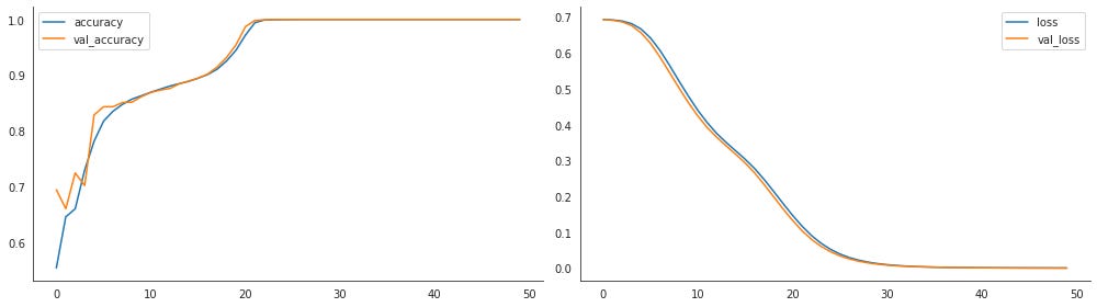
A pair of training-history plots is being created here so the model’s progress over time can be inspected visually. The first line opens a figure with two side-by-side axes, giving room for one plot of accuracy and one plot of loss. Then the stored training history is converted into a table-like DataFrame, and the accuracy and validation accuracy columns are drawn on the left axis. Using the same history data again, the loss and validation loss columns are drawn on the right axis. Because the history object records one value per epoch, each line traces how that metric changed from the start of training to the end.
The saved figure reflects exactly that structure. On the left, both accuracy curves rise quickly and then level off near 1.0, showing that the model learned the classification task very well and that performance on the validation split tracked the training performance closely. On the right, both loss curves fall steadily toward zero, which is what you would expect as the model becomes more confident and makes fewer mistakes. The two lines in each panel stay fairly close together, suggesting that training and validation behavior are similar and there is not much sign of overfitting. The call to remove extra plot borders and tighten the layout just makes the final display cleaner and easier to read.
Retrieve the layer weights
hidden = model.get_layer('hidden').get_weights()This step reaches into the trained network and pulls out the weights from the layer named “hidden.” Keras stores each layer’s learned parameters internally, so after training you can ask the model for a specific layer object and then retrieve its weights. For a dense layer like this one, the returned weights normally come as two arrays: the matrix of connection weights between the input features and the hidden units, and the bias values for each hidden unit. Saving them into a variable makes it possible to inspect how the network has adjusted itself during training, even though nothing is displayed yet. Since the cell only assigns the result to a variable, there is no visible output here; it simply prepares the hidden layer parameters for later examination.
[t.shape for t in hidden][(2, 3), (3,)]This line checks the shapes of the arrays stored in the hidden layer’s weights. Because the hidden layer has 2 inputs and 3 neurons, the weight matrix needs one value for every input-to-neuron connection, which gives a shape of 2 by 3. The second array is the bias vector, and since there is one bias value per neuron, its shape is just 3. The output therefore lists two shapes: one for the connection weights and one for the biases, confirming that the layer contains the expected number of learned parameters.
Visualize the Decision Boundary
The plot of the decision boundary looks much like the one produced by the hand-built network. What stands out, however, is that training with Keras completes several times faster.
n_vals = 200
x1 = np.linspace(-1.5, 1.5, num=n_vals)
x2 = np.linspace(-1.5, 1.5, num=n_vals)
xx, yy = np.meshgrid(x1, x2)  # create the grid
The purpose here is to prepare a regular grid of coordinates that can later be used to probe the model across the two-dimensional input space. A total of 200 values is chosen for each axis, and those values are spread evenly from -1.5 to 1.5 using a linear spacing. That creates two one-dimensional arrays: one for horizontal positions and one for vertical positions.
Those two arrays are then combined into a mesh grid, which turns the separate x and y coordinate lists into two matching 2D arrays. Each position in the first array pairs with each position in the second array, so together they represent every point on a square grid covering the full range. Behind the scenes, this is a convenient way to build a dense set of test points without manually listing them one by one. No output appears because the cell is only setting up these coordinate arrays for a later visualization step, not printing or plotting anything yet.
X_ = np.array([xx.ravel(), yy.ravel()]).TThe purpose of this line is to turn the grid of x and y coordinates into a single list of 2D points that can be fed into the model for prediction. The values xx and yy are typically two matching arrays built from a mesh over the input space, where each pair of entries represents one location on the plane. By flattening both arrays with ravel and then stacking them side by side, the result becomes a two-column array where every row is one point with an x coordinate and a y coordinate. The transpose at the end makes sure the shape is organized the way the model expects: one sample per row, two features per sample.
Behind the scenes, this prepares the full decision surface for evaluation. Instead of predicting only on the original training examples, the model can now make a prediction for every point on the grid. That is what later allows the notebook to color in the background of the plot and show the learned decision boundary across the entire 2D region.
y_hat = np.argmax(model.predict(X_), axis=1)The goal here is to turn the model’s raw probability predictions into a single class label for each input point. The model produces a prediction for both classes at every location in the grid of points being evaluated, so the first step is to run those points through the network and get the output probabilities. Then, for each row of predictions, the highest-probability class is selected. Taking the index of the maximum value across axis 1 means the model’s two output scores are compared for each sample, and whichever class has the larger score becomes the predicted label. The resulting array, y_hat, is therefore a one-dimensional set of class assignments that can be used for plotting the decision regions or comparing the classifier’s choices across the input space. Since this step only computes and stores the predicted labels, there is no visible output in the cell itself.
# Create a color map to show the classification colors of each grid point
cmap = ListedColormap([sns.xkcd_rgb["pale red"],
                       sns.xkcd_rgb["denim blue"]])

# Plot the classification plane with decision boundary and input samples
plt.contourf(xx, yy, y_hat.reshape(n_vals, -1), cmap=cmap, alpha=.25)

# Plot both classes on the x1, x2 plane
data = pd.DataFrame(X, columns=['$x_1$', '$x_2$']).assign(Class=pd.Series(y).map({0:'negative', 1:'positive'}))
sns.scatterplot(x='$x_1$', y='$x_2$', hue='Class', data=data, style=y, markers=['_', '+'], legend=False)
sns.despine()
plt.title('Decision Boundary');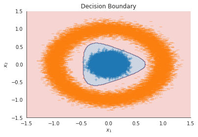
The purpose here is to turn the model’s predictions into a picture of the learned decision boundary and then place the original data points on top so you can judge how well the classifier separated the two classes. First, a two-color map is created so the background of the plot can clearly distinguish the two predicted classes across the 2D input space. The soft red and blue shades are chosen to match the two class regions visually without overpowering the points that will be drawn later.
Next, the code fills in the plane using the model’s predicted class for each point on the grid. The grid values have already been generated elsewhere, and the predictions have been reshaped to match that grid, so each tiny region of the plane can be colored according to which class the model thinks belongs there. The low transparency makes this background visible but still light enough that the real data can stand out on top of it.
After that, the original training data are assembled into a small table with the two input coordinates and a class label. Those labels are turned into readable names, and then a scatter plot is drawn over the background. The styling uses different marker shapes for the two classes, while the hue colors help reinforce which points belong to which class. Because the plot is being shown in a 2D feature space, this overlay directly reveals how the learned boundary relates to the actual circular data.
The saved image shows exactly that result: a soft red background on the outside, a blue region in the middle, and a curved boundary between them. The orange points form the larger outer ring, while the blue points cluster in the center, and the boundary bends around them instead of staying as a straight line. That curved separation is the important visual takeaway, because it shows that the network has learned a nonlinear rule that fits the circle-shaped classes much better than a simple linear model could.
%load_ext tensorboardThis line loads the TensorBoard Jupyter extension into the notebook environment so that TensorBoard can be launched from within the notebook later on. Behind the scenes, it tells Jupyter to register the special TensorBoard commands, which makes the interactive log viewer available without leaving the notebook interface. Since this cell only sets up the extension and does not run a visualization by itself, there is no saved output yet.
%tensorboard --logdir results/tensorboard/<IPython.core.display.HTML object>This launches TensorBoard and points it at the directory where the training logs were written earlier. The log directory contains the files TensorFlow created during model training, such as summaries for loss, accuracy, graphs, and any other tracked information the callback was asked to save. When this command runs inside a Jupyter notebook, it does not print ordinary text output; instead, it creates an embedded browser view so TensorBoard can be opened right inside the notebook.
The saved output reflects that behavior. The HTML object is just the notebook’s internal representation of the embedded display, and the iframe is what actually shows TensorBoard on the page. The script underneath sets the iframe to load the local TensorBoard server, which is typically running on port 6006. That is why the output looks like an empty frame at first: the notebook is preparing a live interactive dashboard, not rendering a static image. Once loaded, TensorBoard can be used to inspect the training curves and other logged results from the model.
Notebook 3 of 5: 03_how_to_use_pytorch
Source file: `03_how_to_use_pytorch_processed.ipynb`
Getting started with PyTorch
PyTorch originated in the Facebook AI Research group under Yann LeCun, and its first alpha release appeared in September 2016. It is built to work closely with Python tools such as NumPy, offers strong support for GPU acceleration, and includes automatic differentiation through its autograd system. Compared with Keras, it gives the user more direct control because it exposes a lower-level API. It is widely used as a research-oriented deep learning framework, and it can also serve as a drop-in alternative to NumPy when GPU computation is needed.
Unlike systems that depend on static computation graphs, such as Theano or TensorFlow, PyTorch uses eager execution. Instead of defining a network ahead of time and compiling it for fixed execution, it performs automatic differentiation through autograd while the tensor operations are being carried out. In other words, gradients are computed as the code runs, which makes it easier to adjust parts of a model dynamically. This programming style is often described as define by run, since the backpropagation behavior follows the actual execution of the code, and each pass through the code can differ. The official documentation includes a thorough tutorial on this approach.
Its blend of flexibility, a Python-centered design, and fast execution has helped PyTorch become widely adopted. That popularity has also encouraged the growth of many companion libraries that broaden what it can do.
Imports and configuration
import warnings
warnings.filterwarnings('ignore')
The purpose of this cell is to keep the notebook output clean by turning off warning messages. Python libraries sometimes emit warnings to point out deprecated features, minor compatibility issues, or other situations that are not fatal errors. By importing the warnings module and setting it to ignore warnings, the notebook stops those messages from appearing during later cells. Since there is no saved output, nothing is displayed here; the effect is purely behind the scenes, making the rest of the notebook easier to read without distracting warning text.
%matplotlib inline

from pprint import pprint

import numpy as np
import pandas as pd

from sklearn.metrics import accuracy_score
from sklearn.datasets import make_circles

import torch
import torch.utils.data as utils
import torch.nn as nn
from torch.autograd import Variable
from livelossplot import PlotLosses

from matplotlib.colors import ListedColormap
import matplotlib.pyplot as plt
import seaborn as sns
This cell sets up the tools the rest of the notebook will rely on. It first tells Jupyter to render plots directly inside the notebook, so any figures created later will appear right below the code instead of in a separate window. After that, it imports a few general-purpose utilities for printing, numerical work, and tabular data handling, along with scikit-learn helpers for measuring accuracy and generating the synthetic two-circle dataset.
The PyTorch imports bring in the main pieces needed for building and training a neural network: the core library, data-loading utilities, and the neural network module collection. The Variable import reflects an older PyTorch style of wrapping tensors, and the live loss plotting package is brought in so training progress can be visualized interactively later on. Finally, the plotting imports prepare the notebook for drawing the decision boundary and data points with customized colors and styling.
There is no saved output from this cell because importing libraries and setting notebook display behavior usually happens quietly. Its role is simply to prepare the environment so the following cells can create data, train the model, and display results without having to repeat these setup steps.
sns.set_style('white')This line changes the default Seaborn plotting style so that future charts use a white background. Behind the scenes, it updates Matplotlib’s style settings through Seaborn, which affects the look of plots created after this point rather than producing any visible output on its own. Because it only sets a global display preference, there is nothing saved in the output area.
input_size = 2         # Input data dimensionality
hidden_size = 3        # The number of nodes at the hidden layer
num_classes = 2        # The number of output classes
num_epochs = 20         # The number of times entire dataset is trained
batch_size = 20        # The size of input data for one iteration
learning_rate = 0.01  # The speed of convergence
This cell sets the basic training settings that the rest of the model will rely on. The first few values describe the shape of the problem and the size of the network: there are two input features, a small hidden layer with three nodes, and two possible output classes. Those numbers need to match the dataset and the model architecture, so they establish the dimensions the network will use when it is built.
The remaining values control how training will proceed. The model will be trained for 20 full passes through the dataset, the data will be processed in batches of 20 samples at a time, and the learning rate is set to 0.01 so the optimizer makes relatively small parameter updates on each step. Nothing is printed here, so there is no saved output; the cell simply prepares these configuration values for later cells that create the network and run the training loop.
Generate the dataset
Generate Synthetic Data
# dataset params
N = 50000
factor = 0.1
noise = 0.1
This step sets the basic parameters for the synthetic dataset that will be created later. The value of N controls how many total samples will be generated, so 50,000 points means the model will have a fairly large training set to learn from. The factor value determines how tightly the two circles are nested inside each other, with a smaller value making the inner circle much smaller relative to the outer one. The noise value adds randomness to the points, so the circles are not perfectly clean and the classification task becomes a little more realistic and slightly harder. Since there is no saved output here, nothing is displayed yet; these lines simply store the chosen dataset settings so the next cell can use them when generating the data.
# generate data
X, y = make_circles(
    n_samples=N,
    shuffle=False,
    factor=factor,
    noise=noise)
The purpose of this step is to create the synthetic dataset that the rest of the notebook will use for training and visualization. A two-class problem is generated with a circular pattern, which is a useful choice because it is simple to describe but not linearly separable, so it gives the neural network something meaningful to learn.
The function is asked to produce a total of N samples, and the samples are not shuffled. Keeping them in order makes the data generation more predictable, which can be helpful for a teaching example. The factor setting controls how tightly the inner circle sits relative to the outer one, and the noise setting adds randomness so the classes are not perfectly clean. That noise makes the task more realistic and prevents the problem from being too trivial.
The result is stored in two arrays: X contains the two-dimensional coordinates for each point, and y contains the corresponding class label for each point. There is no visible output from the cell because its job is simply to prepare data in memory rather than display anything. The generated arrays are then ready to be converted into PyTorch tensors and fed into the training pipeline.
Convert the data into Torch tensors
We start by turning the NumPy or pandas inputs into torch tensors. Moving data back and forth between NumPy and PyTorch is simple:
X_tensor = torch.from_numpy(X)
y_tensor = torch.from_numpy(y)
The purpose here is to take the synthetic data that was created earlier and turn it into PyTorch tensors. That matters because PyTorch works most naturally with its own tensor objects, especially once you want to build a model, compute gradients, and train with the rest of the PyTorch tools.
The first line converts the feature array into a tensor. Those features represent the two input coordinates for each sample, so the resulting tensor keeps the same numeric values and shape, just in a format PyTorch can work with directly. The second line does the same thing for the labels, turning the class targets into a tensor as well. Since no output is saved for this cell, nothing is displayed when it runs; the important effect is that these two tensor variables are now available for the later steps that package the data into a dataset and feed it through a DataLoader during training.
X_tensor.shape, y_tensor.shape(torch.Size([50000, 2]), torch.Size([50000]))The purpose here is to check the size of the two tensors created from the synthetic dataset. The feature tensor has 50,000 rows and 2 columns, which matches the 2D circle data where each sample has two coordinates. The label tensor has 50,000 entries, one class label for each sample. The output confirms that the features and targets are aligned correctly: every point in the dataset has a corresponding label, and the shapes are exactly what the later training code expects.
Build a Torch Dataset
We can first wrap these PyTorch tensors in a TensorDataset and then create a DataLoader that also specifies the batch size:
dataset = utils.TensorDataset(X_tensor,y_tensor)This step bundles the feature tensor and the label tensor into a single dataset object that PyTorch can work with more easily. The features and targets were already converted from NumPy arrays into tensors earlier, and now they are being paired sample by sample so each input point stays matched with its correct class label. Behind the scenes, the dataset object just stores those two tensors together and provides a way to retrieve one training example at a time or in batches later on.
Creating this paired dataset is important because it becomes the foundation for the data-loading pipeline used during training. Once the samples are organized this way, a DataLoader can later read from the dataset, shuffle the examples, and form minibatches automatically. Since there is no saved output here, nothing is displayed yet; the cell simply prepares the data in a format that the next training steps can use.
Set up the Torch DataLoader
dataloader = utils.DataLoader(dataset,
                              batch_size=batch_size,
                              shuffle=True)
This step creates the data loader that will feed training examples to the model in small batches. Rather than handing the entire dataset to the network at once, the data is wrapped so PyTorch can deliver it batch by batch, which is much more efficient and is the standard way to train on larger datasets.
The batch size controls how many samples are grouped together each time the loader yields data. Because shuffling is turned on, the order of the samples will be randomized every time a new pass through the data begins. That randomness matters during training because it helps the model avoid learning patterns tied to the original ordering of the dataset and usually leads to better optimization behavior.
Nothing is printed here, so there is no saved output to interpret. The effect of the cell is simply to prepare a reusable object that the later training loop can iterate over when it needs mini-batches of features and labels.
Construct the Network
Model structure
PyTorch expresses a neural network by building a custom Net() class. The key method is forward, which describes how data moves through the model. Once that forward pass is defined, autograd can automatically construct the matching backward pass and calculate gradients for the parameters.
The forward method is not limited to a narrow set of operations. Any valid Tensor operation can be used there, which gives PyTorch a great deal of freedom in model design. In this example, the implementation is intentionally simple: after setting up the layer attributes, the Tensor is passed through a sequence of straightforward input and output transformations.
class Net(nn.Module):
    def __init__(self, input_size, hidden_size, num_classes):
        super(Net, self).__init__()                    # Inherited from the parent class nn.Module
        self.fc1 = nn.Linear(input_size, hidden_size)
        self.logistic = nn.LogSigmoid()
        self.fc2 = nn.Linear(hidden_size, num_classes)
        self.softmax = nn.Softmax(dim=1)

    def forward(self, x):
        """Forward pass: stacking each layer together"""
        out = self.fc1(x)
        out = self.logistic(out)
        out = self.fc2(out)
        out = self.softmax(out)
        return out
A small neural network is being defined here as a reusable PyTorch model class. The goal is to describe the model’s structure once so it can later be instantiated and trained on the dataset. By inheriting from PyTorch’s module base class, the network automatically fits into PyTorch’s system for tracking parameters, computing gradients, and switching between training and evaluation behavior.
The initialization step sets up the layers the model will use. First, a linear layer takes the two input features and maps them into a hidden representation with three units. Then a LogSigmoid activation is inserted to introduce nonlinearity, which is what allows the network to learn more than a straight line decision rule. After that, another linear layer maps the hidden values to the two output classes. A softmax layer is placed at the end so the final outputs can be interpreted as class probabilities that sum to one across the two classes.
The forward method defines the exact path data takes through the model when a batch is passed in. The input moves through the first linear transformation, then through the nonlinear activation, then through the second linear layer, and finally through softmax. PyTorch uses this forward pass to build the computation graph behind the scenes, so when training begins it will know how to propagate gradients backward through each operation automatically.
There is no saved output because the cell only defines the model; it does not run any data through it yet. The visible effect of executing it is that the Net class becomes available for later use, so a network can be created, trained, and asked to make predictions.
net = Net(input_size, hidden_size, num_classes)
net
Net(
(fc1): Linear(in_features=2, out_features=3, bias=True)
(logistic): LogSigmoid()
(fc2): Linear(in_features=3, out_features=2, bias=True)
(softmax): Softmax(dim=1)
)A new instance of the neural network is created here using the chosen input size, hidden size, and number of output classes. That means the model is being set up with two input features, a small hidden layer of three neurons, and two output units for the binary classification task. Because the network is built as a PyTorch module, creating it also initializes the learnable weights and biases inside each layer.
The next line asks Jupyter to display the model object, so the saved output is a textual summary of its structure. That summary shows the first linear layer mapping from 2 inputs to 3 hidden units, followed by a LogSigmoid activation, then a second linear layer mapping from 3 hidden units to 2 outputs, and finally a Softmax layer applied across the class dimension. The printed representation is useful because it confirms the model has been assembled correctly and makes the architecture easy to inspect at a glance before training begins.
pprint(list(net.parameters()))[Parameter containing:
tensor([[-0.0076, -0.1194],
[-0.1808, -0.5467],
[ 0.3306, -0.6842]], requires_grad=True),
Parameter containing:
tensor([-0.1182, 0.4586, 0.3842], requires_grad=True),
Parameter containing:
tensor([[ 0.4405, -0.1387, 0.1524],
[-0.4791, -0.0536, 0.5147]], requires_grad=True),
Parameter containing:
tensor([ 0.4601, -0.1767], requires_grad=True)]The purpose here is to inspect the model’s learned parameters so far, right after the network has been defined and before or during training. By turning the parameter iterator into a list and sending it to pretty-printing, the notebook makes the weights and biases visible in a readable way instead of leaving them hidden inside the model object. That is a useful sanity check because it shows exactly what the optimizer will update during training.
The output contains four parameter tensors, which matches the two linear layers in the network. The first tensor is the weight matrix for the first linear layer, and its shape reflects the fact that the model takes 2 input features and maps them to 3 hidden units. The next tensor is the bias vector for that same layer, with one bias value for each hidden unit. The third tensor is the weight matrix for the second linear layer, connecting the 3 hidden units to the 2 output classes. The final tensor is the bias vector for the output layer.
Each parameter is marked as requiring gradients, which is exactly what we want in a trainable neural network. That flag tells PyTorch’s autograd system to keep track of these values during the forward pass so it can compute gradients for them during backpropagation. The specific numbers shown are small random initial values rather than anything meaningful yet, which is why they look arbitrary and unstructured. They are simply the starting point that training will gradually adjust.
list(net.parameters())[0]Parameter containing:
tensor([[-0.0076, -0.1194],
[-0.1808, -0.5467],
[ 0.3306, -0.6842]], requires_grad=True)The cell is simply looking at the first learnable tensor inside the network, which is the weight matrix of the first linear layer. PyTorch stores a model’s adjustable values as parameters, and calling the parameter list lets you inspect them directly. Since the first layer maps the 2 input features into 3 hidden units, this weight tensor has three rows and two columns, with each row holding the two weights feeding into one hidden neuron.
The saved output shows the current values of those weights after training. The small positive and negative numbers reflect how the model has adapted its first layer to start separating the two classes. The fact that requires_grad=True appears in the output is important: it means PyTorch is tracking this tensor so gradients can still be computed for it during backpropagation if training continues.
Turn on GPU support
To run the model on a GPU, call net.cuda(). The PyTorch documentation explains how to move tensors to the CPU, a single GPU, or multiple GPUs.
# net.cuda()This line is a reminder that the model can be moved from the CPU to a GPU if one is available. The hash at the start means it is commented out, so it does nothing when the cell runs. If it were enabled, the network and its parameters would be transferred to CUDA memory so later training and inference could run on the graphics card instead of the processor. That is often much faster for neural network workloads, especially when there are many batches or a larger model, but it also requires a compatible GPU and the proper PyTorch CUDA setup. Since there is no saved output, the practical result here is simply that nothing changes at execution time; the cell is acting as a note about an optional hardware acceleration step rather than an active operation.
Set Up the Loss Function
We still need to set up a loss function and an optimizer, and we can do that with a few of the built-in choices:
criterion = nn.CrossEntropyLoss()This line sets up the loss function the model will use during training. Cross-entropy loss is the standard choice for classification tasks like this one because it measures how far the model’s predicted class probabilities are from the true class labels. Behind the scenes, PyTorch will use this criterion to compare the network’s output for each batch against the correct answers and produce a single number that represents the training error. That number is what the optimizer will try to reduce by adjusting the network’s weights. Since there is no saved output, the cell is simply preparing an important training component rather than displaying anything on screen.
Choose the Optimizer
optimizer = torch.optim.Adam(net.parameters(), lr=learning_rate)This line sets up the optimizer, which is the part of training that actually adjusts the model’s weights after the loss has been computed and gradients have been backpropagated. Here, Adam is chosen, one of the most commonly used optimization algorithms in deep learning because it combines momentum-like behavior with adaptive learning rates for each parameter. The model’s parameters are passed in so the optimizer knows exactly which values it is allowed to update, and the learning rate controls how large each step should be when it moves those parameters in the direction suggested by the gradients. Since the cell produces no saved output, its effect is entirely in preparing the training process: after this line runs, the model is ready to be trained using Adam in the upcoming loop.
Fit the Model
Simple Training Run
Model training is organized as two nested loops. The outer loop corresponds to one epoch, meaning one complete pass through the training set. Inside that, the inner loop iterates over the minibatches returned by the DataLoader. Together, these loops carry out the forward computation and the backward gradient update step used by the learning procedure. It is also important to make sure the data are cast to the right types for the objects and functions being used. For example, the labels must be integers, while the input features should be floating-point values:
for epoch in range(num_epochs):
    print(epoch)
    for i, (features, label) in enumerate(dataloader):

        features = Variable(features.float())
        label = Variable(label.long())

        # Initialize the hidden weights
        optimizer.zero_grad()

        # Forward pass: compute output given features
        outputs = net(features)

        # Compute the loss
        loss = criterion(outputs, label)
        # Backward pass: compute the gradients
        loss.backward()
        # Update the weights
        optimizer.step()
0
1
2
3
4
5
6
7
8
9
10
11
12
13
14
15
16
17
18
19The purpose of this cell is to train the neural network for a set number of epochs using minibatches from the DataLoader. The outer loop steps through the full training process one epoch at a time, and the printed numbers in the saved output show that progression clearly: the model runs through epochs 0 to 19, matching the 20 training passes defined earlier.
At the start of each epoch, the epoch number is printed so you can see training advance in the notebook output. Then the inner loop pulls batches of features and labels from the DataLoader. Each batch is converted into the right PyTorch data types before being used: the input features become floating-point values because neural networks perform their computations in floating point, and the labels become long integers because the loss function expects class indices in that format. Wrapping them in Variable reflects older PyTorch style, but the main idea is simply to prepare the tensors for automatic differentiation and training.
Next, the optimizer’s gradients are cleared. That step is important because PyTorch accumulates gradients by default, so without resetting them the gradients from earlier batches would keep piling up and interfere with learning. After that, the features are passed through the network to produce predictions. Those predictions are compared with the true labels using the loss function, which measures how far the model’s outputs are from the correct classes. Once the loss is computed, backpropagation calculates gradients for every learnable parameter in the network, and the optimizer uses those gradients to update the weights. Repeating this batch by batch, epoch by epoch, gradually helps the model learn the decision boundary for the classification task.
The saved output is just the stream of epoch numbers printed during training, so it does not show the loss or accuracy directly. Instead, it confirms that the loop completed all 20 epochs successfully, with each number marking one full pass through the training data.
Showing loss values as training progresses
The example below shows how to use the livelossplot package to display training losses as the model learns, in a way similar to the built-in behavior Keras provides.
liveloss = PlotLosses()
for epoch in range(num_epochs):
    print(epoch)
    logs = {}
    running_loss = 0.0
    running_corrects = 0
    for i, (features, label) in enumerate(dataloader):

        features = Variable(features.float())
        label = Variable(label.long())

        # Intialize the hidden weight to all zeros
        optimizer.zero_grad()

        # Forward pass: compute the output class given a image
        outputs = net(features)

        # Compute the loss: difference between the output class and the pre-given label
        loss = criterion(outputs, label)
        # Backward pass: compute the weight
        loss.backward()
        # Optimizer: update the weights of hidden nodes
        optimizer.step()

        _, preds = torch.max(outputs, 1)
        running_loss += loss.detach() * features.size(0)
        running_corrects += torch.sum(preds == label.data)

        epoch_loss = running_loss / len(dataset)
        epoch_acc = running_corrects.float() / len(dataloader.dataset)
        logs['log loss'] = loss.item()
        logs['accuracy'] = epoch_acc.item()

    liveloss.update(logs)
    liveloss.draw()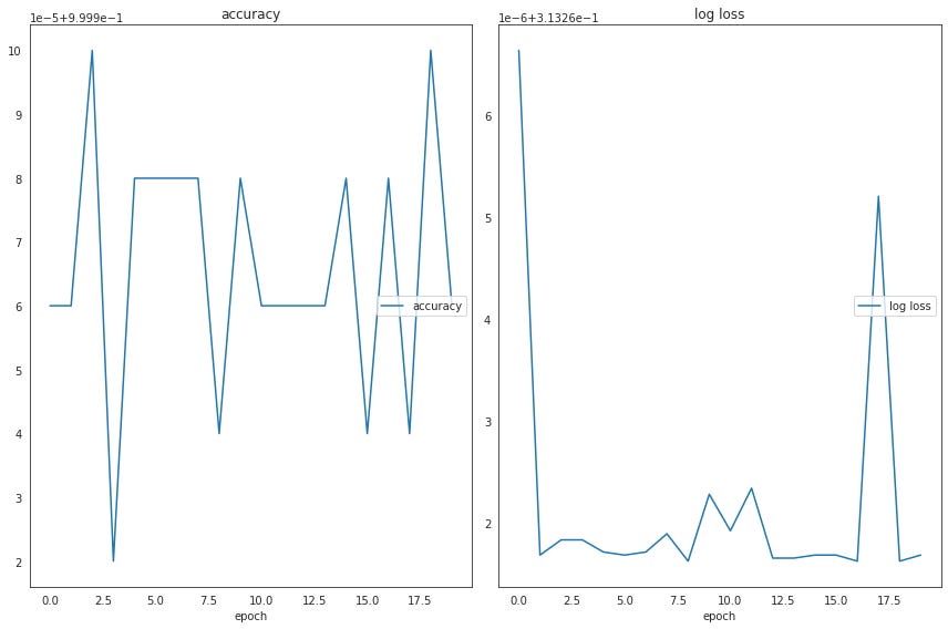
accuracy
	accuracy         	 (min:    1.000, max:    1.000, cur:    1.000)
log loss
	log loss         	 (min:    0.313, max:    0.313, cur:    0.313)
The goal here is to run another training pass over the model while watching its behavior live. A live loss tracker is created first, and then the model is trained for the full number of epochs using minibatches from the data loader. At the start of each epoch, the epoch number is printed, and a fresh set of logging values is prepared so the code can keep track of how training is going.
Inside the batch loop, the feature tensors are converted to floating point and the labels are converted to integer class indices, which is what the loss function expects. Before each update, the optimizer clears out any gradients left over from the previous batch. Then the data is sent through the network to produce outputs, the loss is computed by comparing those outputs with the true labels, and backpropagation calculates gradients for every learnable parameter. After that, the optimizer uses those gradients to adjust the weights.
The code also measures performance as it goes. It picks the predicted class for each example by taking the larger of the two output scores, then compares those predictions with the true labels to accumulate both the running loss and the number of correct predictions. From those totals, it computes an epoch-level loss and accuracy, and stores the most recent values in the logging dictionary.
Once the epoch finishes, the live plotter receives the latest logs and redraws the training curves. That is why the saved output shows a figure with two panels: one for accuracy and one for log loss. The command-line text above the plots reports the latest tracked values as well. The accuracy is displayed as 1.000, which means the model is classifying the training samples perfectly at this point, while the loss is around 0.313, showing that the predicted probabilities are still not infinitely confident even though the class decisions are correct. The plots themselves look a little noisy because the figures are being updated as training progresses, and the scales are very tight, so even small changes in the logged values create visible wiggles.
Make predictions
To generate predictions from the trained model, we feed in the feature data and then turn the result into a NumPy array. The output gives the softmax probability for each of the two classes:
test_value = Variable(torch.from_numpy(X)).float()
prediction = net(test_value).data.numpy()
The purpose here is to run the trained network on the full set of input points and turn its results into a NumPy array that can be worked with outside of PyTorch. First, the feature matrix is converted from a NumPy array into a Torch tensor, wrapped in a Variable, and cast to floating point so it matches the type expected by the model. That step matters because neural networks in PyTorch operate on tensors, and the linear layers inside the network require floating-point inputs. Then the tensor is passed through the model to produce predictions for every sample in X.
Behind the scenes, the network applies its learned weights and activations to each input row and produces output scores for the two classes. The .data part detaches the result from the autograd system, which is a way of saying the prediction values are being treated as plain numbers rather than something the framework should continue tracking for gradient computation. Finally, those values are converted into a NumPy array so they can be used with standard Python and scientific computing tools such as accuracy calculations or plotting. Since there is no saved output, the main effect of running the cell is to prepare prediction values for the next evaluation step.
prediction.shape(50000, 2)This line checks the shape of the model’s prediction array so you can confirm how many samples were processed and how many values were produced for each one. The result shown as (50000, 2) means there is one row for each of the 50,000 data points and two columns for the two class scores or probabilities. That matches the binary classification setup: for every input point, the network returns a pair of outputs, one for each class. Seeing this shape is a useful sanity check because it tells you the prediction step worked as expected and produced an output aligned with the dataset size and the number of classes.
From this point onward, the same workflow can be used to calculate loss measures or to plot the outcome again, which recreates the decision boundary shown earlier.
Evaluate the Predictions
accuracy_score(y_true=y, y_pred=np.argmax(prediction, axis=1))1.0The purpose here is to measure how well the trained model classified the dataset. The saved output of 1.0 means the predicted labels matched the true labels for every example, so the accuracy is perfect on this data.
The calculation works by taking the model’s prediction scores for each sample and converting them into a single class choice with argmax along the class axis. That picks whichever class received the higher probability or score for each point. Those predicted class indices are then compared with the true labels using the accuracy metric, which simply counts the fraction of correct matches.
Because the result is 1.0, the model got every training example right. That makes sense in a setting where the network has already been trained on this same dataset and the problem is relatively simple and synthetic, so the learned decision boundary can separate the two classes very effectively.
Plot the Decision Boundary
Construct the Feature Space
n_vals = 200
x1 = np.linspace(-1.5, 1.5, num=n_vals)
x2 = np.linspace(-1.5, 1.5, num=n_vals)
xx, yy = np.meshgrid(x1, x2)  # create the grid
The purpose here is to set up a regular grid of points across the two-dimensional input space so the model can later be evaluated everywhere on that plane. The first line chooses how fine the grid will be by setting the number of values to 200, which gives enough resolution for a smooth visualization without becoming too expensive to compute. The next two lines create evenly spaced values from -1.5 to 1.5 for each axis, covering the same range in both directions so the plot will be square and centered around the region where the data lives.
After that, the two one-dimensional arrays are combined into a full mesh grid. This turns the single list of x-values and the single list of y-values into two 2D arrays, one containing all the horizontal coordinates and the other containing all the vertical coordinates. Behind the scenes, each pair of matching positions in these arrays represents one point on the plane. That grid is what makes it possible to feed a dense set of coordinates into the network later and see how it classifies different parts of the space.
There is no saved output because nothing is being displayed yet. The cell simply prepares the coordinate system that the later prediction and plotting steps will use to draw the decision boundary.
X_test = np.array([xx.ravel(), yy.ravel()]).T
X_test = torch.from_numpy(X_test)
X_test.shape
torch.Size([40000, 2])The purpose of this step is to turn the two coordinate grids used for plotting into a long list of individual points that can be passed through the neural network. The meshgrid arrays contain a full square of x and y locations, but the model expects one input row per point, with two features in each row. Flattening both grids and stacking them side by side creates exactly that kind of table, where each row represents one location in the plane.
After that, the NumPy array is converted into a PyTorch tensor so it can be used in the same way as the training data was. That matters because the network was built in PyTorch and expects tensor inputs. The final line asks for the tensor’s shape, and the saved output shows torch.Size([40000, 2]). That tells us there are 40,000 grid points in total, each with 2 coordinates. The number 40,000 comes from the mesh resolution: the grid is dense enough to give a smooth decision boundary later, and the two columns confirm that each point still has the x and y values the model needs.
Predict Across the Feature Space
zz = net(Variable(X_test).float()).data.numpy()
zz.shape
(40000, 2)The purpose here is to run the trained neural network on every point in the dense grid used for the decision-boundary plot, then check the shape of the resulting predictions. The grid points are stored in X_test, and they are first wrapped as a Variable and converted to floating-point values so they match the input type the network expects. Passing them through net produces, for each grid point, a pair of output values corresponding to the two classes. The result is then moved out of PyTorch into a NumPy array so it can be handled easily with the plotting tools used later.
The saved output shows that the prediction array has shape (40000, 2). That means there are 40,000 grid points in the mesh, and for each one the model returns two class scores or probabilities. This shape is exactly what you would expect from evaluating a two-class classifier over a flattened 2D grid: one row per point, and one column per class. It confirms that the network has produced a full set of predictions ready to be reshaped back into the grid form needed for the contour plot.
# Create a color map to show the classification colors of each grid point
cmap = ListedColormap([sns.xkcd_rgb["pale red"],
                       sns.xkcd_rgb["denim blue"]])
A two-color map is being prepared here so the later decision-boundary plot can shade each region according to the predicted class. The two colors are pulled from Seaborn’s named XKCD palette, which gives a soft red for one class and a denim blue for the other. Wrapping them in a ListedColormap tells Matplotlib to treat the colors as a fixed set of discrete categories rather than as a smooth gradient, which is exactly what you want for a classification map. Nothing is displayed yet, because this step is only defining the palette that will be reused when the grid of predictions is plotted.
Visualize the decision boundary
# Plot the classification plane with decision boundary and input samples
plt.contourf(xx, yy, np.argmax(zz, axis=1).reshape(n_vals, -1), cmap=cmap, alpha=.25)

# Plot both classes on the x1, x2 plane
data = pd.DataFrame(X, columns=['$x_1$', '$x_2$']).assign(Class=pd.Series(y).map({0:'negative', 1:'positive'}))
sns.scatterplot(x='$x_1$', y='$x_2$', hue='Class', data=data, style=y, markers=['_', '+'], legend=False)
plt.title('Decision Boundary');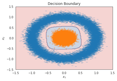
The purpose of this cell is to turn the model’s predictions into a visual decision boundary and then place the original training samples on top so you can see how well the classifier has learned the shape of the problem. The first line uses the grid of points that was evaluated earlier and converts the model’s class probabilities into a single class label for each point by taking the larger of the two predicted values. That label map is reshaped back into the same two-dimensional layout as the mesh grid, and then filled contours are drawn with a transparent color map. Behind the scenes, this creates a shaded background over the plane, where each region represents the class the network would predict for points in that area.
After the background is drawn, the original dataset is assembled into a table with the two input coordinates and a human-readable class name. The labels are mapped from numeric values into the words “negative” and “positive,” which makes the scatter plot easier to interpret. Seaborn then plots the samples on top of the contour map, using different marker styles for the two classes and suppressing the legend so the figure stays uncluttered. The title is added at the end to label the visualization.
The saved figure shows exactly the result of those steps: a colored decision region in the background, with the two concentric classes overlaid as scattered points. The model has learned a curved boundary that separates the inner cluster from the outer ring, so the plot makes it easy to see both the learned classification surface and how the training samples fall within it.
Notebook 4 of 5: 04_optimizing_a_NN_architecture_for_trading
Source file: `04_optimizing_a_NN_architecture_for_trading_processed.ipynb`
Train a deep neural network to forecast asset price returns
In real-world use, it is usually necessary to test several design choices rather than relying on a single assumed architecture, since the best fit for a given dataset is rarely obvious in advance.
This section examines different ways to construct a basic feedforward neural network for predicting asset price returns one day ahead.
Imports and configuration
import warnings
warnings.filterwarnings('ignore')
The purpose here is to quiet down Python’s warning messages so they do not clutter the notebook output. Warnings are often useful during development because they can point out deprecated functions, unstable behavior, or other issues that may need attention, but they can also become distracting when the goal is to focus on the main results of an experiment. By setting the warning filter to ignore, the notebook tells Python to suppress those messages from this point onward. Since the cell only changes how warnings are displayed and does not run any calculation or print anything, there is no visible output afterward.
%matplotlib inline

import os, sys
from ast import literal_eval as make_tuple
from time import time
from pathlib import Path
from itertools import product
import numpy as np
import pandas as pd
import matplotlib.pyplot as plt
import statsmodels.api as sm
from scipy.stats import spearmanr
import seaborn as sns

from sklearn.preprocessing import StandardScaler

import tensorflow as tf
from tensorflow.keras.models import Sequential
from tensorflow.keras.layers import Dense, Dropout, Activation
The cell sets up the notebook environment for the neural-network experiments that follow. It first enables inline plotting so any figures created later will appear directly inside the notebook rather than in a separate window. After that, it brings in the standard tools needed for the rest of the workflow: operating system and path utilities for working with files and directories, a helper for turning text into tuples, timing support for measuring run time, itertools for generating combinations of hyperparameters, and the main scientific Python libraries for numerical work, data handling, plotting, statistics, and visualization.
A few of the imports are especially important for the modeling task. StandardScaler will later be used to normalize the feature values before training, which is a common step for neural networks because they tend to train more reliably when inputs are on comparable scales. TensorFlow and the Keras objects are also loaded here, since they provide the machinery for building the feedforward network itself. Sequential is the model container, while Dense, Dropout, and Activation are the basic building blocks used to stack fully connected layers, apply regularization, and choose nonlinear transformations. Because this cell only prepares the environment and defines no calculations or display commands, there is no saved output, which is exactly what you would expect.
gpu_devices = tf.config.experimental.list_physical_devices('GPU')
if gpu_devices:
    print('Using GPU')
    tf.config.experimental.set_memory_growth(gpu_devices[0], True)
else:
    print('Using CPU')
Using CPUThe purpose here is to check what kind of hardware TensorFlow can use before any model training begins. It first asks TensorFlow for the list of available GPU devices on the system. If that list is not empty, the notebook would announce that a GPU is being used and turn on memory growth for the first GPU, which tells TensorFlow to allocate GPU memory gradually as needed instead of grabbing it all at once. That can help avoid memory-related issues when working with other processes or when the exact memory needs are not known in advance.
Because no GPU is detected, the logic falls into the alternative branch and reports that the CPU will be used instead. The saved output shows exactly that message, which means TensorFlow did not find any compatible GPU device in the environment at runtime. In practice, that means all later model training and inference in the notebook will run on the processor rather than on specialized GPU hardware, which is usually slower but still fully functional.
sys.path.insert(1, os.path.join(sys.path[0], '..'))
from utils import MultipleTimeSeriesCV, format_time
This step prepares the notebook to use helper tools that live outside the standard Python library. First, it adjusts the import search path so that Python will look one level above the current directory when trying to find modules. That matters because the utilities needed here are stored in a local file rather than installed as a package. After that path update, the notebook imports two custom helpers: one is a specialized cross-validation splitter designed for time-ordered financial data, and the other is a small formatting function for turning elapsed time into a readable display. There is no visible output because nothing is being computed or displayed yet; the cell is simply setting up access to functionality that later cells will rely on.
np.random.seed(42)
sns.set_style('whitegrid')
idx = pd.IndexSlice
The purpose of this cell is to set up a predictable and consistent working environment before any modeling or plotting happens. First, the random number generator is seeded with a fixed value so that any later operation that relies on randomness will produce the same results each time the notebook is run. That matters for reproducibility, especially when models are trained, data are shuffled, or parameter combinations are sampled in different orders.
Next, the plotting style is changed to a whitegrid theme, which gives future charts a cleaner background with light grid lines. That makes figures easier to read and compare, particularly for time series or performance plots. Nothing is drawn yet, so there is no saved output, but the visual style setting quietly affects all later plots in the notebook.
Finally, an IndexSlice shortcut is created from pandas. This is a convenience tool for selecting pieces of a multi-indexed DataFrame more easily later on, especially when filtering by combinations of dates and symbols. It does not produce visible output either; it simply prepares a shorthand that will make later data slicing statements shorter and clearer.
DATA_STORE = '../data/assets.h5'This line sets up a file path that points to an HDF5 data store named assets.h5 in a parent data directory. It acts as a convenient reference for later cells so the notebook can open the same dataset without repeating the full path each time. Nothing is loaded or displayed yet, so there is no visible output. The statement simply stores the location as a variable, making the data source easy to reuse if the notebook needs to read from that file later.
results_path = Path('results')
if not results_path.exists():
    results_path.mkdir()

checkpoint_path = results_path / 'logs'
The purpose here is to make sure the folder structure for the experiment exists before any model training or saving begins. First, a path object is created for a directory named results, which is where later outputs such as scores, plots, and prediction files will be stored. The next step checks whether that directory is already present on disk. If it is missing, the directory is created so the notebook will not run into file-saving errors later.
After that, a second path is defined for a logs subfolder inside results. This subfolder is intended for checkpoint files, which are the saved model weights written during training. Nothing is written yet, so there is no visible output from the cell. Its role is simply preparatory: it sets up the locations that later cells will use when they need to persist training progress and experiment results.
Build a stock return series for forecasting asset price changes
To build the trading strategy, we rely on daily stock returns for about 995 US stocks over the eight-year span from 2010 through 2017. We combine these returns with the Chapter 12 feature set, which includes volatility and momentum measures, along with lagged returns ranked both across the full cross-section and within sectors.
data = pd.read_hdf('../12_gradient_boosting_machines/data.h5', 'model_data').dropna().sort_index()The first step is to load the prepared modeling dataset from the HDF5 file used earlier in the workflow. The data are read under the key for the main model table, then any rows with missing values are removed so the later training and evaluation steps work with a clean set of observations. After that, the rows are sorted by their index, which is important when the data are organized by time and asset because later time-series operations assume the records are in a consistent order. Nothing is displayed here because the cell is simply preparing the dataset in memory, so its effect is to set up a clean, ordered DataFrame for the next steps rather than to produce visible output.
data.info(show_counts=True)<class 'pandas.core.frame.DataFrame'>
MultiIndex: 1911344 entries, ('A', Timestamp('2010-04-06 00:00:00')) to ('ZION', Timestamp('2017-11-29 00:00:00'))
Data columns (total 34 columns):
# Column Non-Null Count Dtype
--- ------ -------------- -----
0 dollar_vol 1911344 non-null float64
1 dollar_vol_rank 1911344 non-null float64
2 rsi 1911344 non-null float64
3 bb_high 1911344 non-null float64
4 bb_low 1911344 non-null float64
5 NATR 1911344 non-null float64
6 ATR 1911344 non-null float64
7 PPO 1911344 non-null float64
8 MACD 1911344 non-null float64
9 sector 1911344 non-null int64
10 r01 1911344 non-null float64
11 r05 1911344 non-null float64
12 r10 1911344 non-null float64
13 r21 1911344 non-null float64
14 r42 1911344 non-null float64
15 r63 1911344 non-null float64
16 r01dec 1911344 non-null float64
17 r05dec 1911344 non-null float64
18 r10dec 1911344 non-null float64
19 r21dec 1911344 non-null float64
20 r42dec 1911344 non-null float64
21 r63dec 1911344 non-null float64
22 r01q_sector 1911344 non-null float64
23 r05q_sector 1911344 non-null float64
24 r10q_sector 1911344 non-null float64
25 r21q_sector 1911344 non-null float64
26 r42q_sector 1911344 non-null float64
27 r63q_sector 1911344 non-null float64
28 r01_fwd 1911344 non-null float64
29 r05_fwd 1911344 non-null float64
30 r21_fwd 1911344 non-null float64
31 year 1911344 non-null int64
32 month 1911344 non-null int64
33 weekday 1911344 non-null int64
dtypes: float64(30), int64(4)
memory usage: 503.9+ MBThe purpose here is to take a quick inventory of the dataset before any modeling happens, so you can confirm its shape, indexing, column types, and whether anything is missing. When the dataframe’s info summary is printed, it shows that the data is organized as a MultiIndex with 1,911,344 rows, running from ticker A on 2010-04-06 through ticker ZION on 2017-11-29. That tells you immediately this is panel data: many securities observed across many dates.
The column listing confirms that the table contains 34 variables in total. Most of them are floating-point features, which is what you would expect for market indicators, returns, and transformed return features. A few columns are integers, including the sector label and the calendar-time fields for year, month, and weekday. Seeing the non-null counts all match the total row count is especially useful, because it shows that every column is fully populated here, so there are no missing values to impute or filter out before training. The memory usage line at the end also gives a sense of scale: this is a fairly large dataframe, taking about 504 MB in memory, which explains why later steps like cross-validation and repeated model fitting will be computationally expensive.
outcomes = data.filter(like='fwd').columns.tolist()The cell is identifying which columns in the dataset represent future return targets. It looks through the data and keeps only the column names that contain the string indicating a forward-looking return, then converts that filtered set into a regular Python list. The result is stored for later use as the collection of outcome variables, which makes it easier to separate prediction targets from the feature columns. Since the cell only creates this list and does not print anything or display a table, there is no saved output.
lookahead = 1
outcome= f'r{lookahead:02}_fwd'
This cell sets up the prediction target for the model. It first chooses a one-day lookahead, meaning the model will be trained to predict what happens on the next trading day rather than several days or weeks ahead. From that number, it then builds the name of the outcome column in the dataset by formatting the lookahead as a two-digit value and attaching the forward-return label. With a lookahead of 1, the resulting target name becomes the one-day forward return field, which is the variable the later modeling steps will use as the response. Since the cell only assigns these values and does not display anything, there is no visible output.
X_cv = data.loc[idx[:, :'2017'], :].drop(outcomes, axis=1)
y_cv = data.loc[idx[:, :'2017'], outcome]
The cell prepares the modeling data for cross-validation by splitting the full dataset into input features and the prediction target, while also restricting both to the historical period through 2017. It uses the multi-index on the data to select all symbols but only dates up to and including 2017, which keeps the later evaluation focused on past information rather than more recent observations. From that filtered slice, the first line removes all outcome columns so only the explanatory variables remain in the feature set used for training and validation. The second line pulls out the single target series identified earlier, which is the one-day-ahead return the model is meant to predict. Since the cell only assigns these two objects and does not print, plot, or return anything, there is no saved output.
len(X_cv.index.get_level_values('symbol').unique())995The cell checks how many distinct assets are represented in the cross-validation dataset by taking the unique values from the symbol level of the index and counting them. Because the data is organized as a panel, each symbol corresponds to one asset or stock, so this count tells us how broad the universe is. The result, 995, means there are 995 different symbols included in the modeling sample. That number is useful for understanding the scale of the dataset and how many separate asset histories the model is learning from across the time periods used in training and validation.
X_cv.info(null_counts=True)<class 'pandas.core.frame.DataFrame'>
MultiIndex: 1911344 entries, ('A', Timestamp('2010-04-06 00:00:00')) to ('ZION', Timestamp('2017-11-29 00:00:00'))
Data columns (total 31 columns):
# Column Non-Null Count Dtype
--- ------ -------------- -----
0 dollar_vol 1911344 non-null float64
1 dollar_vol_rank 1911344 non-null float64
2 rsi 1911344 non-null float64
3 bb_high 1911344 non-null float64
4 bb_low 1911344 non-null float64
5 NATR 1911344 non-null float64
6 ATR 1911344 non-null float64
7 PPO 1911344 non-null float64
8 MACD 1911344 non-null float64
9 sector 1911344 non-null int64
10 r01 1911344 non-null float64
11 r05 1911344 non-null float64
12 r10 1911344 non-null float64
13 r21 1911344 non-null float64
14 r42 1911344 non-null float64
15 r63 1911344 non-null float64
16 r01dec 1911344 non-null float64
17 r05dec 1911344 non-null float64
18 r10dec 1911344 non-null float64
19 r21dec 1911344 non-null float64
20 r42dec 1911344 non-null float64
21 r63dec 1911344 non-null float64
22 r01q_sector 1911344 non-null float64
23 r05q_sector 1911344 non-null float64
24 r10q_sector 1911344 non-null float64
25 r21q_sector 1911344 non-null float64
26 r42q_sector 1911344 non-null float64
27 r63q_sector 1911344 non-null float64
28 year 1911344 non-null int64
29 month 1911344 non-null int64
30 weekday 1911344 non-null int64
dtypes: float64(27), int64(4)
memory usage: 460.1+ MBThe purpose here is to inspect the feature matrix being used for model training and make sure it is fully populated and structured the way the later neural network workflow expects. Calling the DataFrame’s info display gives a compact inventory of the dataset: how many rows it contains, how the index is organized, which columns are present, what types they have, and whether any values are missing.
The output shows that the data is indexed by a MultiIndex with 1,911,344 rows, running from the earliest asset-date pair through the latest one shown. That tells us this is panel-style market data, where each row corresponds to one stock on one trading day. There are 31 feature columns in total, covering things like volume, technical indicators, past-return measures, sector identity, and simple calendar variables such as year, month, and weekday. The fact that every column reports the full number of non-null values means the matrix is complete at this stage, so there are no missing entries left to interfere with scaling, cross-validation, or neural network training. The mix of float64 and int64 types also shows that most inputs are continuous numerical features, with a few integer-coded categorical or date-related fields. The large memory usage confirms that this is a substantial dataset, which explains why the later modeling steps rely on careful time-based splits and efficient training rather than simple one-shot fitting.
Automate model creation
The make_model function below shows how the architecture search can be configured in a flexible way. The dense_layers argument supplies a list of integers that determines both how many hidden layers the network has and how many units each layer contains. Dropout is included as a regularization setting and is given as a decimal between 0 and 1, representing the chance that a unit will be omitted during a training step.
def make_model(dense_layers, activation, dropout):
    '''Creates a multi-layer perceptron model

    dense_layers: List of layer sizes; one number per layer
    '''

    model = Sequential()
    for i, layer_size in enumerate(dense_layers, 1):
        if i == 1:
            model.add(Dense(layer_size, input_dim=X_cv.shape[1]))
            model.add(Activation(activation))
        else:
            model.add(Dense(layer_size))
            model.add(Activation(activation))
    model.add(Dropout(dropout))
    model.add(Dense(1))

    model.compile(loss='mean_squared_error',
                  optimizer='Adam')

    return model
This cell sets up a reusable recipe for building a feedforward neural network, so later experiments can create many different model variants without rewriting the architecture each time. The function takes three choices as inputs: the sizes of the hidden layers, the activation function to apply after each layer, and the dropout rate to use near the end.
The model is constructed layer by layer using a sequential stack, which means each layer feeds directly into the next. For the first hidden layer, the network also needs to know the number of input features, so the function uses the width of the training feature matrix to set that input size. After that first layer, the same activation function is applied, and the pattern repeats for any additional hidden layers listed in the layer-size sequence. This makes the function flexible enough to handle shallow or deeper networks with different widths.
Once the hidden layers are in place, the model adds dropout, which randomly switches off a fraction of units during training to reduce overfitting and encourage the network to learn more robust patterns. The final layer has a single output neuron because the task is to predict one continuous value: the next-day return. The model is then compiled with mean squared error as the loss function, which is standard for regression, and Adam as the optimizer, which will handle the weight updates during training.
There is no saved output from the cell because nothing is being trained or displayed yet. The cell simply defines the function so that it can be called later to generate specific model versions for the different hyperparameter combinations.
Evaluate several model settings with TensorFlow through cross-validation
Splitting the Data into Training and Test Sets
We divide the sample so that cross-validation is done on the training portion, while the most recent 12 months of available observations are reserved as the holdout test set:
n_splits = 12
train_period_length=21 * 12 * 4
test_period_length=21 * 3
This cell sets the basic time-series cross-validation schedule that will be used later in the experiment. It chooses 12 separate splits, which means the model will be evaluated repeatedly on different train-and-test windows rather than on one single division of the data. The training window is defined as 21 trading days times 12 months times 4 years, so each fold uses about four years of daily data for fitting the model. The test window is set to 21 trading days times 3 months, which gives roughly one quarter of a year for validation in each split.
Nothing is displayed because the cell only assigns values to variables. Those settings are important behind the scenes because they control how much history the model sees before each validation period and how long each out-of-sample evaluation period lasts. Later cells use these numbers when the rolling time-series splitter is created, so this small setup step determines the structure of the entire cross-validation procedure.
cv = MultipleTimeSeriesCV(n_splits=n_splits,
                          train_period_length=train_period_length,
                          test_period_length=test_period_length,
                          lookahead=lookahead)
This cell sets up the time-based cross-validation scheme that will be used for the model experiment. Instead of splitting the data randomly, it creates a custom splitter designed for financial time series, where preserving chronological order matters. The number of folds, the length of each training window, the length of each validation window, and the one-day lookahead are all passed in here so the splitter knows exactly how to carve the historical data into rolling train-and-test periods.
Behind the scenes, this object does not train anything yet or produce predictions. It simply prepares the rules for how the data will be divided later on, making sure each validation fold comes after its corresponding training fold in time. That setup is essential for avoiding look-ahead bias and for getting a realistic estimate of how the model might perform on future data. Since the cell only creates the splitter and does not print or display anything, there is no visible output when it runs.
Set up the cross-validation settings
Now we only need to set up the Keras model with make_model, configure cross-validation with the OneStepTimeSeriesSplit approach discussed in chapter 6 on The Machine Learning Process and the sections that follow, and specify the hyperparameters for the search.
The experiment considers a handful of network layouts with one or two hidden layers, together with both relu and tanh activations and several dropout settings. It would also be reasonable to test alternative optimizers, but that variation was left out so the study would stay within the bounds of an already expensive computation.
dense_layer_opts = [(16, 8), (32, 16), (32, 32), (64, 32)]
activation_opts = ['tanh']
dropout_opts = [0, .1, .2]
The purpose here is to set up the search space for the neural network experiment by defining which architectural choices will be tried later. One list contains the possible pairs of hidden-layer sizes, so each option represents a two-layer feedforward network with different widths. Another list fixes the activation function choices, and here only one activation is included, so every model in this stage will use the same nonlinearity. A third list specifies the dropout rates to test, ranging from no dropout to moderate regularization.
Nothing is displayed because the cell is only creating these option lists in memory. The lack of output is exactly what you would expect: there is no calculation to summarize yet, just a small configuration step that prepares the combinations for the upcoming model runs.
param_grid = list(product(dense_layer_opts, activation_opts, dropout_opts))
np.random.shuffle(param_grid)
The purpose of this cell is to build the list of neural network configurations that will be tested later and then randomize their order. It starts by combining the available choices for layer sizes, activation functions, and dropout rates into every possible parameter combination. Each combination represents one candidate model setup, so turning those options into a full grid gives the search procedure a clear set of architectures to try.
After that, the order of the combinations is shuffled. That does not change which models will be evaluated, but it does change the sequence in which they are visited. Shuffling is useful because it prevents the experiment from always running the settings in the same fixed order, which can make the search feel more balanced and can help avoid any unintended dependence on ordering. Since the cell only prepares a Python list in memory and does not print anything or create a figure, there is no saved output.
len(param_grid)12The cell is checking how many hyperparameter combinations are in the search space. Since the earlier setup builds a list of model settings by combining the available layer configurations, activation choice, and dropout rates, taking the length of that list gives the total number of distinct model variants that will be tried. The result, 12, reflects the full set of combinations currently defined in the grid, so it confirms that the experiment will evaluate a dozen different configurations rather than just a small handful or an empty set.
To start the hyperparameter search, we create a GridSearchCV instance, set the fit_params that will be forwarded to the Keras model’s fit call, and then supply the training data when calling fit on the GridSearchCV object:
def get_train_valid_data(X, y, train_idx, test_idx):
    x_train, y_train = X.iloc[train_idx, :], y.iloc[train_idx]
    x_val, y_val = X.iloc[test_idx, :], y.iloc[test_idx]
    return x_train, y_train, x_val, y_val
A small helper function is being set up here to make the cross-validation loop easier to read and reuse. Its job is simply to take the full feature table and target series, along with two sets of row positions that mark the training period and the validation period, and split the data into the four pieces needed for model fitting and evaluation.
The function pulls the training features and targets from the rows indicated by the training indices, then does the same for the validation rows. Because the data is stored in pandas objects, it uses positional selection, which means the split follows the exact index positions produced by the time-series cross-validation scheme rather than any label-based lookup. That matters in a financial time-series setting, where preserving the intended order of observations is essential and random shuffling would break the logic of the evaluation.
At the end, the function returns the four subsets in a fixed order: training features, training targets, validation features, and validation targets. There is no saved output because nothing is meant to be displayed yet; the cell only defines a reusable utility that later cells can call repeatedly during model training and testing.
ic = []
scaler = StandardScaler()
for params in param_grid:
    dense_layers, activation, dropout = params
    for batch_size in [64, 256]:
        print(dense_layers, activation, dropout, batch_size)
        checkpoint_dir = checkpoint_path / str(dense_layers) / activation / str(dropout) / str(batch_size)
        if not checkpoint_dir.exists():
            checkpoint_dir.mkdir(parents=True, exist_ok=True)
        start = time()
        for fold, (train_idx, test_idx) in enumerate(cv.split(X_cv)):
            # get train & validation data
            x_train, y_train, x_val, y_val = get_train_valid_data(X_cv, y_cv, train_idx, test_idx)

            # scale features
            x_train = scaler.fit_transform(x_train)
            x_val = scaler.transform(x_val)

            # set up dataframes to log results
            preds = y_val.to_frame('actual')
            r = pd.DataFrame(index=y_val.groupby(level='date').size().index)

            # create model based on validation parameters
            model = make_model(dense_layers, activation, dropout)

            # cross-validate for 20 epochs
            for epoch in range(20):
                model.fit(x_train,
                          y_train,
                          batch_size=batch_size,
                          epochs=1,
                          verbose=0,
                          shuffle=True,
                          validation_data=(x_val, y_val))
                model.save_weights((checkpoint_dir / f'ckpt_{fold}_{epoch}').as_posix())
                preds[epoch] = model.predict(x_val).squeeze()
                r[epoch] = preds.groupby(level='date').apply(lambda x: spearmanr(x.actual, x[epoch])[0]).to_frame(epoch)
                print(format_time(time()-start), f'{fold + 1:02d} | {epoch + 1:02d} | {r[epoch].mean():7.4f} | {r[epoch].median():7.4f}')
            ic.append(r.assign(dense_layers=str(dense_layers),
                               activation=activation,
                               dropout=dropout,
                               batch_size=batch_size,
                               fold=fold))

        t = time()-start
        pd.concat(ic).to_hdf(results_path / 'scores.h5', 'ic_by_day')
(64, 32) tanh 0.1 64
00:00:10 01 | 01 | -0.0051 | 0.0013
00:00:18 01 | 02 | 0.0002 | -0.0062
00:00:26 01 | 03 | 0.0110 | -0.0003
00:00:34 01 | 04 | 0.0144 | 0.0097
00:00:42 01 | 05 | 0.0070 | 0.0061
00:00:50 01 | 06 | 0.0289 | 0.0227
00:00:59 01 | 07 | 0.0156 | 0.0342
00:01:07 01 | 08 | 0.0090 | 0.0127
00:01:15 01 | 09 | 0.0084 | 0.0096
00:01:23 01 | 10 | 0.0172 | 0.0296
00:01:31 01 | 11 | 0.0165 | 0.0217
00:01:39 01 | 12 | 0.0016 | 0.0086
00:01:47 01 | 13 | 0.0191 | 0.0344
00:01:55 01 | 14 | 0.0088 | 0.0064
00:02:03 01 | 15 | 0.0058 | 0.0121
00:02:10 01 | 16 | 0.0203 | 0.0227
00:02:18 01 | 17 | 0.0220 | 0.0177
00:02:26 01 | 18 | 0.0140 | 0.0083
00:02:34 01 | 19 | -0.0011 | 0.0009
00:02:41 01 | 20 | 0.0048 | 0.0015
00:02:50 02 | 01 | 0.0008 | -0.0016
00:02:58 02 | 02 | -0.0116 | -0.0011
00:03:06 02 | 03 | 0.0050 | 0.0096
00:03:14 02 | 04 | -0.0017 | 0.0076
00:03:22 02 | 05 | -0.0000 | -0.0086
00:03:30 02 | 06 | 0.0187 | 0.0401
00:03:39 02 | 07 | -0.0055 | 0.0081
00:03:48 02 | 08 | 0.0009 | 0.0016
00:03:57 02 | 09 | 0.0085 | 0.0039
00:04:05 02 | 10 | -0.0056 | 0.0070
00:04:13 02 | 11 | 0.0095 | 0.0083
00:04:21 02 | 12 | 0.0073 | -0.0036
00:04:29 02 | 13 | 0.0066 | 0.0119
00:04:38 02 | 14 | -0.0019 | 0.0046
00:04:46 02 | 15 | -0.0227 | -0.0106
00:04:54 02 | 16 | 0.0030 | 0.0049
00:05:03 02 | 17 | -0.0115 | 0.0013
00:05:11 02 | 18 | -0.0062 | -0.0058
00:05:19 02 | 19 | 0.0136 | 0.0137
00:05:28 02 | 20 | 0.0096 | -0.0055
00:05:37 03 | 01 | 0.0217 | 0.0118
00:05:45 03 | 02 | 0.0093 | 0.0221
00:05:54 03 | 03 | 0.0027 | -0.0191
00:06:02 03 | 04 | 0.0124 | 0.0063
00:06:10 03 | 05 | 0.0031 | -0.0039
00:06:18 03 | 06 | -0.0156 | -0.0395
00:06:27 03 | 07 | 0.0055 | -0.0013
00:06:35 03 | 08 | 0.0029 | -0.0028
00:06:43 03 | 09 | 0.0149 | 0.0163
00:06:52 03 | 10 | -0.0103 | -0.0060
00:07:00 03 | 11 | -0.0265 | -0.0366
00:07:09 03 | 12 | -0.0069 | -0.0074
00:07:17 03 | 13 | -0.0134 | -0.0183
00:07:26 03 | 14 | 0.0097 | -0.0067
00:07:34 03 | 15 | -0.0076 | -0.0049
00:07:43 03 | 16 | -0.0045 | -0.0078
00:07:52 03 | 17 | 0.0106 | 0.0109
00:08:00 03 | 18 | -0.0216 | -0.0197
00:08:09 03 | 19 | -0.0024 | 0.0017
00:08:17 03 | 20 | -0.0069 | 0.0007
00:08:27 04 | 01 | -0.0329 | -0.0321
00:08:36 04 | 02 | -0.0085 | -0.0062
00:08:44 04 | 03 | 0.0070 | 0.0038
00:08:53 04 | 04 | -0.0123 | -0.0092
00:09:01 04 | 05 | 0.0141 | 0.0021
00:09:10 04 | 06 | 0.0397 | 0.0368
00:09:19 04 | 07 | 0.0160 | 0.0159
00:09:27 04 | 08 | -0.0166 | -0.0049
00:09:36 04 | 09 | 0.0055 | 0.0045
00:09:45 04 | 10 | -0.0035 | -0.0133
00:09:54 04 | 11 | 0.0236 | 0.0080
00:10:04 04 | 12 | -0.0068 | -0.0152
00:10:13 04 | 13 | 0.0244 | 0.0329
00:10:21 04 | 14 | 0.0323 | 0.0091
00:10:30 04 | 15 | 0.0189 | 0.0187
00:10:39 04 | 16 | 0.0270 | 0.0115
00:10:47 04 | 17 | -0.0091 | -0.0087
00:10:56 04 | 18 | -0.0217 | -0.0162
00:11:04 04 | 19 | -0.0476 | -0.0535
00:11:13 04 | 20 | 0.0248 | 0.0033
00:11:23 05 | 01 | 0.0176 | 0.0181
00:11:31 05 | 02 | -0.0133 | -0.0183
00:11:40 05 | 03 | -0.0115 | -0.0144
00:11:48 05 | 04 | 0.0149 | 0.0123
00:11:57 05 | 05 | 0.0087 | -0.0025
00:12:06 05 | 06 | 0.0086 | 0.0118
00:12:14 05 | 07 | -0.0032 | 0.0227
00:12:23 05 | 08 | 0.0021 | 0.0031
00:12:31 05 | 09 | -0.0196 | -0.0109
00:12:40 05 | 10 | 0.0011 | 0.0049
00:12:49 05 | 11 | -0.0096 | -0.0101
00:12:57 05 | 12 | -0.0137 | -0.0151
00:13:06 05 | 13 | 0.0036 | -0.0083
00:13:14 05 | 14 | 0.0038 | 0.0103
00:13:23 05 | 15 | -0.0090 | -0.0090
00:13:32 05 | 16 | -0.0110 | -0.0237
00:13:41 05 | 17 | -0.0170 | -0.0163
00:13:51 05 | 18 | -0.0208 | -0.0472
00:14:00 05 | 19 | -0.0158 | -0.0416
00:14:09 05 | 20 | 0.0097 | 0.0196
00:14:21 06 | 01 | 0.0160 | 0.0209
00:14:32 06 | 02 | 0.0311 | 0.0189
00:14:42 06 | 03 | 0.0388 | 0.0232
00:14:53 06 | 04 | 0.0287 | 0.0140
00:15:04 06 | 05 | 0.0378 | 0.0338
00:15:14 06 | 06 | 0.0268 | 0.0211
00:15:24 06 | 07 | 0.0351 | 0.0266
00:15:34 06 | 08 | 0.0492 | 0.0299
00:15:45 06 | 09 | 0.0553 | 0.0358
00:15:55 06 | 10 | 0.0231 | 0.0139
00:16:04 06 | 11 | 0.0509 | 0.0549
00:16:14 06 | 12 | 0.0290 | 0.0130
00:16:22 06 | 13 | 0.0461 | 0.0541
00:16:30 06 | 14 | 0.0447 | 0.0471
00:16:39 06 | 15 | 0.0285 | 0.0269
00:16:47 06 | 16 | 0.0316 | 0.0406
00:16:55 06 | 17 | 0.0375 | 0.0297
00:17:04 06 | 18 | 0.0189 | 0.0198
00:17:12 06 | 19 | 0.0335 | 0.0258
00:17:20 06 | 20 | 0.0124 | -0.0001
00:17:30 07 | 01 | -0.0086 | -0.0051
00:17:38 07 | 02 | -0.0330 | -0.0368
00:17:47 07 | 03 | -0.0102 | -0.0093
00:17:56 07 | 04 | 0.0154 | 0.0268
00:18:04 07 | 05 | 0.0167 | 0.0251
00:18:13 07 | 06 | 0.0351 | 0.0209
00:18:22 07 | 07 | 0.0137 | 0.0346
00:18:31 07 | 08 | 0.0083 | 0.0199
00:18:40 07 | 09 | 0.0123 | 0.0327
00:18:50 07 | 10 | 0.0364 | 0.0644
00:19:00 07 | 11 | 0.0114 | 0.0116
00:19:10 07 | 12 | 0.0249 | 0.0406
00:19:19 07 | 13 | 0.0299 | 0.0380
00:19:28 07 | 14 | 0.0158 | 0.0409
00:19:37 07 | 15 | 0.0211 | 0.0420
00:19:46 07 | 16 | 0.0051 | 0.0080
00:19:55 07 | 17 | 0.0242 | 0.0081
00:20:03 07 | 18 | -0.0091 | 0.0219
00:20:11 07 | 19 | 0.0396 | 0.0253
00:20:19 07 | 20 | 0.0252 | 0.0255
00:20:28 08 | 01 | 0.0348 | 0.0529
00:20:36 08 | 02 | -0.0048 | -0.0090
00:20:44 08 | 03 | 0.0302 | 0.0346
00:20:52 08 | 04 | 0.0105 | 0.0146
00:21:01 08 | 05 | 0.0065 | 0.0023
00:21:09 08 | 06 | 0.0241 | 0.0294
00:21:16 08 | 07 | 0.0250 | 0.0208
00:21:24 08 | 08 | 0.0042 | 0.0219
00:21:32 08 | 09 | 0.0050 | -0.0004
00:21:40 08 | 10 | 0.0101 | 0.0002
00:21:48 08 | 11 | 0.0219 | 0.0306
00:21:56 08 | 12 | 0.0137 | 0.0259
00:22:04 08 | 13 | 0.0141 | 0.0153
00:22:13 08 | 14 | 0.0269 | 0.0201
00:22:21 08 | 15 | 0.0081 | -0.0028
00:22:29 08 | 16 | 0.0133 | 0.0099
00:22:37 08 | 17 | 0.0124 | 0.0181
00:22:46 08 | 18 | 0.0182 | 0.0367
00:22:54 08 | 19 | 0.0112 | 0.0293
00:23:01 08 | 20 | 0.0403 | 0.0490
00:23:11 09 | 01 | -0.0044 | -0.0233
00:23:19 09 | 02 | 0.0210 | 0.0274
00:23:27 09 | 03 | 0.0336 | 0.0255
00:23:35 09 | 04 | 0.0127 | 0.0014
00:23:43 09 | 05 | 0.0193 | 0.0180
00:23:51 09 | 06 | 0.0131 | 0.0102
00:23:59 09 | 07 | 0.0206 | 0.0308
00:24:07 09 | 08 | 0.0191 | 0.0124
00:24:15 09 | 09 | 0.0213 | 0.0235
00:24:24 09 | 10 | 0.0131 | 0.0110
00:24:32 09 | 11 | 0.0084 | 0.0018
00:24:40 09 | 12 | 0.0042 | 0.0007
00:24:47 09 | 13 | 0.0243 | 0.0269
00:24:56 09 | 14 | 0.0093 | 0.0106
00:25:04 09 | 15 | 0.0063 | 0.0068
00:25:12 09 | 16 | 0.0095 | 0.0176
00:25:20 09 | 17 | 0.0043 | 0.0161
00:25:28 09 | 18 | 0.0029 | 0.0048
00:25:36 09 | 19 | -0.0015 | -0.0024
00:25:44 09 | 20 | 0.0021 | 0.0113
00:25:53 10 | 01 | -0.0095 | -0.0189
00:26:01 10 | 02 | 0.0327 | 0.0359
00:26:09 10 | 03 | -0.0115 | -0.0056
00:26:17 10 | 04 | -0.0210 | -0.0314
00:26:25 10 | 05 | 0.0008 | -0.0059
00:26:33 10 | 06 | 0.0245 | 0.0065
00:26:41 10 | 07 | 0.0302 | 0.0283
00:26:49 10 | 08 | 0.0057 | 0.0047
00:26:57 10 | 09 | -0.0075 | -0.0049
00:27:05 10 | 10 | -0.0072 | 0.0029
00:27:13 10 | 11 | 0.0265 | 0.0271
00:27:21 10 | 12 | 0.0139 | 0.0329
00:27:29 10 | 13 | 0.0153 | 0.0079
00:27:37 10 | 14 | 0.0189 | 0.0076
00:27:45 10 | 15 | -0.0021 | -0.0152
00:27:53 10 | 16 | 0.0116 | -0.0136
00:28:01 10 | 17 | -0.0029 | -0.0053
00:28:09 10 | 18 | 0.0194 | 0.0204
00:28:17 10 | 19 | -0.0092 | -0.0084
00:28:25 10 | 20 | 0.0312 | 0.0170
00:28:34 11 | 01 | 0.0142 | 0.0038
00:28:42 11 | 02 | 0.0042 | 0.0061
00:28:50 11 | 03 | 0.0084 | 0.0100
00:28:59 11 | 04 | 0.0112 | 0.0030
00:29:07 11 | 05 | 0.0169 | 0.0115
00:29:15 11 | 06 | 0.0274 | 0.0276
00:29:22 11 | 07 | 0.0251 | 0.0199
00:29:30 11 | 08 | 0.0311 | 0.0261
00:29:39 11 | 09 | 0.0182 | 0.0143
00:29:47 11 | 10 | 0.0286 | 0.0286
00:29:55 11 | 11 | -0.0030 | -0.0153
00:30:03 11 | 12 | 0.0414 | 0.0329
00:30:11 11 | 13 | 0.0234 | 0.0162
00:30:19 11 | 14 | 0.0320 | 0.0298
00:30:27 11 | 15 | 0.0307 | 0.0260
00:30:35 11 | 16 | 0.0298 | 0.0339
00:30:43 11 | 17 | -0.0007 | -0.0005
00:30:51 11 | 18 | 0.0156 | 0.0121
00:30:59 11 | 19 | 0.0222 | 0.0177
00:31:08 11 | 20 | 0.0231 | 0.0143
00:31:17 12 | 01 | 0.0076 | 0.004500:31:25 12 | 02 | 0.0133 | 0.0058
00:31:33 12 | 03 | 0.0094 | 0.0001
00:31:41 12 | 04 | 0.0163 | 0.0168
00:31:49 12 | 05 | 0.0046 | 0.0050
00:31:57 12 | 06 | 0.0111 | 0.0386
00:32:05 12 | 07 | 0.0046 | -0.0144
00:32:14 12 | 08 | 0.0085 | 0.0197
00:32:22 12 | 09 | 0.0056 | -0.0001
00:32:30 12 | 10 | -0.0037 | -0.0360
00:32:38 12 | 11 | 0.0078 | 0.0028
00:32:46 12 | 12 | 0.0073 | 0.0035
00:32:54 12 | 13 | 0.0026 | 0.0058
00:33:02 12 | 14 | 0.0100 | 0.0128
00:33:10 12 | 15 | -0.0003 | 0.0002
00:33:18 12 | 16 | -0.0034 | -0.0100
00:33:26 12 | 17 | -0.0009 | -0.0083
00:33:34 12 | 18 | -0.0100 | -0.0172
00:33:42 12 | 19 | -0.0097 | -0.0171
00:33:51 12 | 20 | -0.0114 | -0.0260
(64, 32) tanh 0.1 256
00:00:05 01 | 01 | 0.0119 | -0.0027
00:00:08 01 | 02 | 0.0188 | 0.0172
00:00:11 01 | 03 | 0.0018 | 0.0017
00:00:15 01 | 04 | 0.0083 | 0.0137
00:00:18 01 | 05 | -0.0015 | 0.0026
00:00:21 01 | 06 | 0.0061 | 0.0183
00:00:24 01 | 07 | -0.0106 | -0.0080
00:00:28 01 | 08 | 0.0195 | 0.0237
00:00:31 01 | 09 | -0.0051 | -0.0121
00:00:34 01 | 10 | 0.0137 | 0.0162
00:00:38 01 | 11 | 0.0146 | 0.0191
00:00:41 01 | 12 | 0.0203 | 0.0295
00:00:44 01 | 13 | 0.0105 | 0.0181
00:00:48 01 | 14 | 0.0119 | 0.0123
00:00:51 01 | 15 | 0.0081 | 0.0031
00:00:54 01 | 16 | 0.0090 | 0.0019
00:00:58 01 | 17 | 0.0098 | 0.0137
00:01:01 01 | 18 | 0.0088 | 0.0059
00:01:04 01 | 19 | 0.0109 | 0.0118
00:01:08 01 | 20 | 0.0010 | 0.0009
00:01:12 02 | 01 | 0.0033 | -0.0003
00:01:15 02 | 02 | 0.0095 | 0.0368
00:01:19 02 | 03 | -0.0104 | -0.0189
00:01:22 02 | 04 | -0.0133 | -0.0014
00:01:25 02 | 05 | 0.0102 | -0.0033
00:01:28 02 | 06 | 0.0209 | 0.0483
00:01:32 02 | 07 | 0.0106 | 0.0025
00:01:35 02 | 08 | -0.0120 | -0.0291
00:01:38 02 | 09 | -0.0005 | 0.0020
00:01:42 02 | 10 | 0.0010 | 0.0020
00:01:45 02 | 11 | -0.0005 | 0.0014
00:01:48 02 | 12 | 0.0136 | 0.0156
00:01:52 02 | 13 | 0.0176 | 0.0111
00:01:55 02 | 14 | 0.0028 | -0.0083
00:01:58 02 | 15 | 0.0096 | 0.0233
00:02:02 02 | 16 | -0.0039 | -0.0022
00:02:05 02 | 17 | 0.0006 | 0.0081
00:02:08 02 | 18 | -0.0033 | -0.0034
00:02:12 02 | 19 | -0.0078 | -0.0064
00:02:15 02 | 20 | 0.0129 | -0.0009
00:02:19 03 | 01 | 0.0006 | -0.0078
00:02:23 03 | 02 | 0.0048 | 0.0032
00:02:26 03 | 03 | -0.0025 | -0.0069
00:02:30 03 | 04 | 0.0226 | 0.0300
00:02:33 03 | 05 | -0.0091 | 0.0086
00:02:36 03 | 06 | 0.0097 | 0.0107
00:02:39 03 | 07 | 0.0172 | 0.0217
00:02:43 03 | 08 | 0.0154 | 0.0149
00:02:46 03 | 09 | -0.0200 | -0.0400
00:02:50 03 | 10 | -0.0241 | -0.0427
00:02:54 03 | 11 | -0.0083 | -0.0120
00:02:57 03 | 12 | 0.0004 | -0.0203
00:03:01 03 | 13 | 0.0016 | 0.0004
00:03:05 03 | 14 | -0.0082 | -0.0282
00:03:08 03 | 15 | -0.0004 | -0.0133
00:03:12 03 | 16 | 0.0068 | 0.0135
00:03:15 03 | 17 | -0.0121 | -0.0440
00:03:19 03 | 18 | 0.0043 | -0.0100
00:03:23 03 | 19 | 0.0038 | 0.0052
00:03:26 03 | 20 | 0.0063 | 0.0077
00:03:32 04 | 01 | 0.0207 | 0.0241
00:03:35 04 | 02 | -0.0041 | 0.0075
00:03:39 04 | 03 | -0.0450 | -0.0648
00:03:43 04 | 04 | 0.0087 | -0.0041
00:03:46 04 | 05 | 0.0005 | -0.0241
00:03:50 04 | 06 | -0.0001 | 0.0110
00:03:54 04 | 07 | -0.0117 | -0.0248
00:03:57 04 | 08 | 0.0125 | -0.0197
00:04:01 04 | 09 | 0.0092 | -0.0083
00:04:05 04 | 10 | 0.0229 | 0.0255
00:04:08 04 | 11 | 0.0242 | 0.0063
00:04:12 04 | 12 | -0.0143 | -0.0230
00:04:16 04 | 13 | -0.0222 | -0.0261
00:04:19 04 | 14 | 0.0089 | -0.0113
00:04:23 04 | 15 | 0.0018 | -0.0034
00:04:27 04 | 16 | -0.0018 | 0.0089
00:04:30 04 | 17 | 0.0120 | 0.0029
00:04:34 04 | 18 | -0.0138 | 0.0051
00:04:37 04 | 19 | -0.0272 | -0.0155
00:04:40 04 | 20 | 0.0084 | -0.0157
00:04:44 05 | 01 | -0.0034 | 0.0032
00:04:48 05 | 02 | 0.0233 | 0.0297
00:04:51 05 | 03 | 0.0007 | -0.0147
00:04:55 05 | 04 | 0.0039 | 0.0097
00:04:58 05 | 05 | 0.0140 | 0.0212
00:05:01 05 | 06 | 0.0037 | 0.0037
00:05:05 05 | 07 | -0.0052 | 0.0042
00:05:08 05 | 08 | 0.0100 | 0.0042
00:05:11 05 | 09 | 0.0155 | 0.0222
00:05:15 05 | 10 | 0.0074 | 0.0070
00:05:18 05 | 11 | 0.0063 | 0.0198
00:05:21 05 | 12 | 0.0054 | -0.0035
00:05:24 05 | 13 | 0.0018 | 0.0124
00:05:28 05 | 14 | -0.0037 | 0.0053
00:05:31 05 | 15 | -0.0079 | 0.0036
00:05:34 05 | 16 | 0.0003 | -0.0011
00:05:37 05 | 17 | 0.0006 | -0.0132
00:05:40 05 | 18 | 0.0032 | -0.0006
00:05:44 05 | 19 | -0.0043 | -0.0053
00:05:47 05 | 20 | 0.0035 | 0.0066
00:05:51 06 | 01 | 0.0159 | -0.0027
00:05:55 06 | 02 | -0.0193 | -0.0404
00:05:58 06 | 03 | 0.0241 | 0.0186
00:06:01 06 | 04 | -0.0183 | -0.0256
00:06:05 06 | 05 | 0.0223 | 0.0153
00:06:08 06 | 06 | 0.0295 | 0.0297
00:06:12 06 | 07 | 0.0233 | 0.0397
00:06:16 06 | 08 | 0.0199 | 0.0220
00:06:19 06 | 09 | 0.0224 | 0.0176
00:06:22 06 | 10 | 0.0216 | 0.0288
00:06:25 06 | 11 | 0.0275 | 0.0382
00:06:28 06 | 12 | 0.0174 | -0.0008
00:06:32 06 | 13 | 0.0208 | 0.0278
00:06:35 06 | 14 | 0.0236 | 0.0281
00:06:38 06 | 15 | 0.0142 | 0.0166
00:06:41 06 | 16 | 0.0104 | -0.0084
00:06:45 06 | 17 | 0.0327 | 0.0212
00:06:48 06 | 18 | 0.0080 | 0.0154
00:06:51 06 | 19 | 0.0191 | 0.0286
00:06:55 06 | 20 | 0.0238 | 0.0203
00:06:60 07 | 01 | 0.0196 | 0.0165
00:07:03 07 | 02 | 0.0128 | 0.0306
00:07:06 07 | 03 | 0.0223 | 0.0254
00:07:10 07 | 04 | 0.0194 | 0.0137
00:07:13 07 | 05 | 0.0222 | -0.0005
00:07:16 07 | 06 | 0.0249 | 0.0227
00:07:20 07 | 07 | 0.0362 | 0.0333
00:07:23 07 | 08 | 0.0265 | 0.0638
00:07:26 07 | 09 | 0.0140 | 0.0234
00:07:30 07 | 10 | 0.0088 | -0.0073
00:07:33 07 | 11 | 0.0036 | -0.0019
00:07:37 07 | 12 | 0.0025 | -0.0048
00:07:41 07 | 13 | 0.0299 | -0.0081
00:07:45 07 | 14 | 0.0144 | 0.0038
00:07:48 07 | 15 | 0.0180 | -0.0050
00:07:52 07 | 16 | 0.0166 | -0.0002
00:07:56 07 | 17 | -0.0061 | -0.0225
00:07:59 07 | 18 | 0.0004 | -0.0268
00:08:03 07 | 19 | 0.0114 | -0.0018
00:08:07 07 | 20 | 0.0194 | -0.0033
00:08:11 08 | 01 | 0.0005 | 0.0176
00:08:15 08 | 02 | 0.0077 | 0.0174
00:08:18 08 | 03 | 0.0099 | 0.0030
00:08:22 08 | 04 | 0.0282 | 0.0265
00:08:25 08 | 05 | 0.0358 | 0.0127
00:08:28 08 | 06 | 0.0214 | 0.0228
00:08:32 08 | 07 | 0.0378 | 0.0379
00:08:35 08 | 08 | 0.0026 | 0.0193
00:08:39 08 | 09 | 0.0258 | 0.0073
00:08:42 08 | 10 | 0.0143 | 0.0070
00:08:46 08 | 11 | 0.0150 | 0.0113
00:08:50 08 | 12 | 0.0308 | 0.0253
00:08:53 08 | 13 | 0.0238 | 0.0238
00:08:57 08 | 14 | 0.0239 | 0.0207
00:09:01 08 | 15 | 0.0256 | 0.0302
00:09:04 08 | 16 | 0.0363 | 0.0122
00:09:08 08 | 17 | 0.0315 | 0.0242
00:09:12 08 | 18 | 0.0353 | 0.0207
00:09:15 08 | 19 | 0.0210 | 0.0131
00:09:19 08 | 20 | 0.0141 | 0.0059
00:09:23 09 | 01 | 0.0041 | -0.0001
00:09:27 09 | 02 | -0.0143 | -0.0108
00:09:31 09 | 03 | 0.0030 | -0.0066
00:09:34 09 | 04 | 0.0021 | 0.0035
00:09:38 09 | 05 | 0.0151 | 0.0130
00:09:41 09 | 06 | -0.0010 | -0.0111
00:09:45 09 | 07 | 0.0341 | 0.0414
00:09:49 09 | 08 | 0.0169 | 0.0041
00:09:52 09 | 09 | 0.0259 | 0.0278
00:09:56 09 | 10 | 0.0287 | 0.0204
00:09:59 09 | 11 | 0.0166 | 0.0116
00:10:03 09 | 12 | 0.0189 | 0.0226
00:10:07 09 | 13 | 0.0208 | 0.0218
00:10:10 09 | 14 | 0.0147 | 0.0059
00:10:14 09 | 15 | 0.0158 | 0.0103
00:10:17 09 | 16 | 0.0152 | 0.0178
00:10:21 09 | 17 | 0.0154 | 0.0128
00:10:25 09 | 18 | 0.0192 | 0.0172
00:10:28 09 | 19 | 0.0216 | 0.0297
00:10:32 09 | 20 | 0.0190 | 0.0220
00:10:37 10 | 01 | -0.0383 | -0.0742
00:10:41 10 | 02 | -0.0239 | -0.0390
00:10:45 10 | 03 | 0.0238 | 0.0204
00:10:48 10 | 04 | 0.0198 | 0.0339
00:10:52 10 | 05 | -0.0304 | -0.0322
00:10:55 10 | 06 | -0.0298 | -0.0623
00:10:59 10 | 07 | -0.0490 | -0.0721
00:11:03 10 | 08 | -0.0122 | -0.0267
00:11:06 10 | 09 | -0.0058 | -0.0192
00:11:10 10 | 10 | -0.0216 | -0.0174
00:11:14 10 | 11 | -0.0182 | -0.0363
00:11:17 10 | 12 | -0.0301 | -0.0314
00:11:21 10 | 13 | -0.0158 | -0.0314
00:11:25 10 | 14 | -0.0175 | -0.0284
00:11:28 10 | 15 | -0.0187 | -0.0221
00:11:32 10 | 16 | -0.0207 | -0.0441
00:11:36 10 | 17 | 0.0074 | -0.0023
00:11:39 10 | 18 | 0.0054 | 0.0012
00:11:43 10 | 19 | 0.0041 | 0.0050
00:11:47 10 | 20 | 0.0040 | -0.0033
00:11:51 11 | 01 | -0.0119 | -0.0027
00:11:55 11 | 02 | 0.0309 | 0.036200:11:58 11 | 03 | 0.0428 | 0.0488
00:12:02 11 | 04 | 0.0250 | 0.0235
00:12:06 11 | 05 | 0.0270 | 0.0318
00:12:09 11 | 06 | 0.0335 | 0.0354
00:12:13 11 | 07 | 0.0004 | -0.0036
00:12:17 11 | 08 | -0.0034 | -0.0096
00:12:20 11 | 09 | -0.0067 | -0.0123
00:12:24 11 | 10 | 0.0102 | 0.0104
00:12:27 11 | 11 | 0.0214 | 0.0292
00:12:31 11 | 12 | 0.0237 | 0.0220
00:12:35 11 | 13 | 0.0223 | 0.0176
00:12:38 11 | 14 | 0.0265 | 0.0132
00:12:42 11 | 15 | 0.0206 | 0.0175
00:12:45 11 | 16 | 0.0266 | 0.0145
00:12:49 11 | 17 | 0.0335 | 0.0355
00:12:53 11 | 18 | 0.0210 | 0.0107
00:12:56 11 | 19 | 0.0424 | 0.0297
00:12:60 11 | 20 | 0.0197 | 0.0153
00:13:04 12 | 01 | 0.0070 | 0.0164
00:13:08 12 | 02 | 0.0086 | 0.0021
00:13:11 12 | 03 | 0.0222 | 0.0245
00:13:14 12 | 04 | 0.0098 | -0.0140
00:13:18 12 | 05 | 0.0057 | -0.0068
00:13:21 12 | 06 | 0.0075 | -0.0103
00:13:24 12 | 07 | 0.0223 | 0.0186
00:13:28 12 | 08 | 0.0317 | 0.0217
00:13:31 12 | 09 | 0.0053 | -0.0047
00:13:34 12 | 10 | 0.0149 | -0.0066
00:13:38 12 | 11 | 0.0145 | 0.0028
00:13:41 12 | 12 | 0.0054 | -0.0074
00:13:44 12 | 13 | 0.0070 | -0.0210
00:13:47 12 | 14 | 0.0056 | -0.0104
00:13:51 12 | 15 | 0.0042 | -0.0095
00:13:54 12 | 16 | 0.0135 | 0.0147
00:13:57 12 | 17 | 0.0012 | -0.0201
00:14:01 12 | 18 | 0.0097 | 0.0226
00:14:04 12 | 19 | -0.0076 | -0.0315
00:14:08 12 | 20 | 0.0014 | 0.0070
(64, 32) tanh 0 64
00:00:10 01 | 01 | 0.0016 | 0.0012
00:00:17 01 | 02 | 0.0195 | 0.0222
00:00:25 01 | 03 | 0.0151 | 0.0153
00:00:33 01 | 04 | 0.0063 | 0.0289
00:00:41 01 | 05 | 0.0060 | 0.0056
00:00:49 01 | 06 | 0.0064 | 0.0246
00:00:57 01 | 07 | 0.0143 | 0.0093
00:01:05 01 | 08 | 0.0131 | 0.0169
00:01:13 01 | 09 | 0.0139 | 0.0225
00:01:21 01 | 10 | 0.0143 | 0.0039
00:01:29 01 | 11 | 0.0058 | -0.0056
00:01:38 01 | 12 | 0.0165 | 0.0102
00:01:47 01 | 13 | 0.0122 | 0.0136
00:01:55 01 | 14 | 0.0134 | 0.0250
00:02:04 01 | 15 | 0.0273 | 0.0357
00:02:13 01 | 16 | 0.0100 | 0.0103
00:02:21 01 | 17 | 0.0218 | 0.0276
00:02:29 01 | 18 | 0.0152 | 0.0095
00:02:37 01 | 19 | 0.0124 | 0.0087
00:02:45 01 | 20 | 0.0233 | 0.0118
00:02:55 02 | 01 | -0.0212 | -0.0234
00:03:03 02 | 02 | 0.0220 | 0.0289
00:03:11 02 | 03 | 0.0218 | 0.0163
00:03:19 02 | 04 | -0.0200 | -0.0061
00:03:27 02 | 05 | 0.0004 | -0.0040
00:03:35 02 | 06 | 0.0186 | 0.0151
00:03:43 02 | 07 | 0.0016 | 0.0028
00:03:50 02 | 08 | 0.0013 | 0.0209
00:03:58 02 | 09 | 0.0103 | 0.0183
00:04:06 02 | 10 | -0.0213 | -0.0206
00:04:14 02 | 11 | -0.0017 | -0.0019
00:04:22 02 | 12 | -0.0012 | -0.0186
00:04:30 02 | 13 | 0.0088 | 0.0249
00:04:38 02 | 14 | -0.0045 | -0.0006
00:04:46 02 | 15 | -0.0019 | 0.0055
00:04:53 02 | 16 | 0.0006 | -0.0110
00:05:01 02 | 17 | -0.0068 | -0.0273
00:05:09 02 | 18 | 0.0003 | 0.0113
00:05:17 02 | 19 | 0.0125 | 0.0110
00:05:25 02 | 20 | 0.0152 | 0.0074
00:05:34 03 | 01 | 0.0105 | 0.0090
00:05:41 03 | 02 | -0.0078 | -0.0017
00:05:48 03 | 03 | 0.0369 | 0.0320
00:05:55 03 | 04 | 0.0122 | -0.0140
00:06:03 03 | 05 | -0.0170 | -0.0361
00:06:10 03 | 06 | -0.0162 | -0.0109
00:06:17 03 | 07 | -0.0179 | -0.0384
00:06:24 03 | 08 | -0.0128 | -0.0273
00:06:32 03 | 09 | -0.0322 | -0.0294
00:06:39 03 | 10 | -0.0228 | -0.0239
00:06:46 03 | 11 | 0.0021 | 0.0050
00:06:53 03 | 12 | -0.0006 | 0.0157
00:07:01 03 | 13 | -0.0081 | -0.0233
00:07:08 03 | 14 | -0.0309 | -0.0461
00:07:15 03 | 15 | -0.0189 | -0.0211
00:07:23 03 | 16 | 0.0082 | -0.0084
00:07:30 03 | 17 | -0.0219 | -0.0220
00:07:37 03 | 18 | -0.0239 | -0.0306
00:07:44 03 | 19 | -0.0012 | 0.0113
00:07:52 03 | 20 | 0.0020 | 0.0078
00:07:60 04 | 01 | 0.0167 | 0.0409
00:08:07 04 | 02 | 0.0143 | 0.0168
00:08:14 04 | 03 | -0.0161 | -0.0162
00:08:22 04 | 04 | 0.0268 | 0.0165
00:08:29 04 | 05 | -0.0443 | -0.0348
00:08:36 04 | 06 | -0.0420 | -0.0576
00:08:44 04 | 07 | -0.0334 | -0.0187
00:08:51 04 | 08 | -0.0006 | -0.0090
00:08:58 04 | 09 | -0.0453 | -0.0507
00:09:06 04 | 10 | 0.0099 | -0.0126
00:09:13 04 | 11 | -0.0242 | -0.0041
00:09:20 04 | 12 | -0.0070 | -0.0126
00:09:28 04 | 13 | 0.0136 | -0.0037
00:09:35 04 | 14 | 0.0345 | 0.0238
00:09:42 04 | 15 | 0.0229 | 0.0165
00:09:49 04 | 16 | -0.0497 | -0.0411
00:09:57 04 | 17 | 0.0001 | -0.0113
00:10:04 04 | 18 | 0.0110 | 0.0077
00:10:11 04 | 19 | -0.0425 | -0.0279
00:10:19 04 | 20 | 0.0039 | 0.0218
00:10:27 05 | 01 | -0.0174 | -0.0010
00:10:34 05 | 02 | 0.0148 | 0.0222
00:10:41 05 | 03 | 0.0108 | 0.0154
00:10:49 05 | 04 | 0.0323 | 0.0340
00:10:56 05 | 05 | 0.0103 | -0.0038
00:11:03 05 | 06 | -0.0015 | -0.0033
00:11:10 05 | 07 | 0.0168 | 0.0158
00:11:18 05 | 08 | 0.0239 | 0.0274
00:11:25 05 | 09 | 0.0132 | -0.0091
00:11:32 05 | 10 | 0.0137 | 0.0124
00:11:40 05 | 11 | 0.0196 | 0.0192
00:11:47 05 | 12 | 0.0061 | -0.0096
00:11:54 05 | 13 | -0.0058 | -0.0004
00:12:02 05 | 14 | -0.0042 | 0.0126
00:12:09 05 | 15 | 0.0287 | 0.0240
00:12:16 05 | 16 | 0.0166 | 0.0119
00:12:24 05 | 17 | 0.0031 | 0.0016
00:12:31 05 | 18 | -0.0047 | 0.0047
00:12:38 05 | 19 | 0.0122 | 0.0123
00:12:46 05 | 20 | 0.0178 | 0.0098
00:12:54 06 | 01 | 0.0234 | 0.0198
00:13:01 06 | 02 | -0.0069 | -0.0034
00:13:08 06 | 03 | 0.0339 | 0.0437
00:13:16 06 | 04 | 0.0345 | 0.0147
00:13:23 06 | 05 | 0.0192 | 0.0177
00:13:30 06 | 06 | 0.0283 | 0.0247
00:13:38 06 | 07 | 0.0152 | 0.0085
00:13:45 06 | 08 | -0.0017 | -0.0013
00:13:52 06 | 09 | 0.0248 | 0.0344
00:13:60 06 | 10 | 0.0380 | 0.0185
00:14:07 06 | 11 | 0.0239 | -0.0020
00:14:15 06 | 12 | 0.0205 | -0.0045
00:14:22 06 | 13 | 0.0334 | 0.0297
00:14:30 06 | 14 | 0.0373 | 0.0172
00:14:37 06 | 15 | 0.0447 | 0.0549
00:14:44 06 | 16 | 0.0126 | -0.0000
00:14:52 06 | 17 | 0.0325 | 0.0281
00:14:59 06 | 18 | 0.0258 | 0.0103
00:15:07 06 | 19 | 0.0453 | 0.0691
00:15:14 06 | 20 | 0.0398 | 0.0487
00:15:22 07 | 01 | 0.0218 | 0.0335
00:15:29 07 | 02 | 0.0376 | 0.0496
00:15:37 07 | 03 | 0.0005 | 0.0194
00:15:44 07 | 04 | -0.0230 | -0.0202
00:15:51 07 | 05 | 0.0054 | -0.0225
00:15:58 07 | 06 | 0.0213 | 0.0189
00:16:06 07 | 07 | -0.0081 | -0.0031
00:16:13 07 | 08 | 0.0345 | 0.0605
00:16:20 07 | 09 | 0.0014 | 0.0095
00:16:28 07 | 10 | -0.0074 | -0.0022
00:16:35 07 | 11 | 0.0102 | 0.0215
00:16:42 07 | 12 | 0.0054 | 0.0341
00:16:50 07 | 13 | 0.0229 | 0.0540
00:16:57 07 | 14 | 0.0163 | 0.0621
00:17:04 07 | 15 | -0.0198 | -0.0048
00:17:12 07 | 16 | 0.0189 | 0.0077
00:17:19 07 | 17 | -0.0005 | -0.0056
00:17:26 07 | 18 | 0.0299 | 0.0715
00:17:34 07 | 19 | 0.0366 | 0.0574
00:17:41 07 | 20 | 0.0239 | 0.0205
00:17:49 08 | 01 | -0.0010 | -0.0107
00:17:56 08 | 02 | 0.0019 | -0.0171
00:18:04 08 | 03 | 0.0109 | 0.0008
00:18:11 08 | 04 | 0.0159 | 0.0442
00:18:19 08 | 05 | -0.0102 | 0.0067
00:18:26 08 | 06 | 0.0205 | 0.0224
00:18:33 08 | 07 | 0.0112 | 0.0203
00:18:41 08 | 08 | 0.0158 | 0.0242
00:18:48 08 | 09 | 0.0072 | 0.0030
00:18:55 08 | 10 | 0.0210 | 0.0099
00:19:02 08 | 11 | 0.0023 | -0.0208
00:19:10 08 | 12 | 0.0112 | 0.0316
00:19:17 08 | 13 | 0.0046 | 0.0053
00:19:25 08 | 14 | 0.0075 | -0.0063
00:19:32 08 | 15 | -0.0018 | 0.0064
00:19:39 08 | 16 | 0.0060 | 0.0131
00:19:47 08 | 17 | 0.0179 | 0.0367
00:19:54 08 | 18 | 0.0024 | -0.0092
00:20:01 08 | 19 | 0.0208 | 0.0401
00:20:09 08 | 20 | -0.0006 | 0.0411
00:20:17 09 | 01 | -0.0012 | -0.0071
00:20:24 09 | 02 | 0.0038 | -0.0036
00:20:31 09 | 03 | 0.0082 | 0.0027
00:20:39 09 | 04 | 0.0089 | 0.0183
00:20:46 09 | 05 | 0.0201 | 0.0215
00:20:53 09 | 06 | 0.0156 | 0.0180
00:21:01 09 | 07 | -0.0043 | -0.0049
00:21:08 09 | 08 | 0.0065 | 0.0062
00:21:15 09 | 09 | 0.0012 | 0.0041
00:21:23 09 | 10 | 0.0132 | 0.0014
00:21:30 09 | 11 | 0.0043 | -0.0058
00:21:38 09 | 12 | -0.0094 | -0.0182
00:21:45 09 | 13 | -0.0059 | -0.0146
00:21:52 09 | 14 | -0.0026 | -0.0131
00:21:60 09 | 15 | 0.0005 | 0.0004
00:22:07 09 | 16 | 0.0003 | -0.0028
00:22:15 09 | 17 | -0.0010 | 0.0043
00:22:22 09 | 18 | -0.0137 | -0.0131
00:22:29 09 | 19 | 0.0014 | 0.0089
00:22:37 09 | 20 | 0.0033 | 0.0015
00:22:45 10 | 01 | -0.0230 | -0.0269
00:22:52 10 | 02 | -0.0310 | -0.0773
00:22:59 10 | 03 | -0.0068 | 0.002700:23:07 10 | 04 | -0.0260 | -0.0485
00:23:14 10 | 05 | 0.0051 | -0.0052
00:23:21 10 | 06 | -0.0108 | -0.0292
00:23:28 10 | 07 | -0.0013 | -0.0012
00:23:36 10 | 08 | -0.0218 | -0.0377
00:23:43 10 | 09 | -0.0052 | -0.0046
00:23:50 10 | 10 | -0.0053 | -0.0111
00:23:57 10 | 11 | -0.0169 | -0.0131
00:24:05 10 | 12 | -0.0201 | -0.0271
00:24:12 10 | 13 | 0.0050 | 0.0089
00:24:19 10 | 14 | -0.0045 | 0.0041
00:24:26 10 | 15 | 0.0085 | 0.0154
00:24:34 10 | 16 | -0.0027 | -0.0020
00:24:41 10 | 17 | -0.0173 | 0.0048
00:24:48 10 | 18 | -0.0182 | 0.0004
00:24:55 10 | 19 | -0.0078 | 0.0018
00:25:03 10 | 20 | -0.0054 | 0.0090
00:25:11 11 | 01 | 0.0045 | 0.0087
00:25:18 11 | 02 | 0.0319 | 0.0106
00:25:26 11 | 03 | 0.0077 | 0.0156
00:25:33 11 | 04 | -0.0020 | -0.0110
00:25:40 11 | 05 | 0.0203 | 0.0222
00:25:47 11 | 06 | 0.0049 | 0.0032
00:25:55 11 | 07 | 0.0258 | 0.0155
00:26:02 11 | 08 | 0.0159 | 0.0122
00:26:10 11 | 09 | 0.0094 | 0.0003
00:26:17 11 | 10 | 0.0219 | 0.0125
00:26:24 11 | 11 | 0.0274 | 0.0277
00:26:32 11 | 12 | 0.0230 | 0.0202
00:26:39 11 | 13 | 0.0156 | 0.0208
00:26:46 11 | 14 | 0.0057 | -0.0018
00:26:54 11 | 15 | 0.0167 | 0.0158
00:27:01 11 | 16 | 0.0133 | 0.0009
00:27:08 11 | 17 | 0.0063 | -0.0000
00:27:16 11 | 18 | 0.0163 | 0.0135
00:27:23 11 | 19 | 0.0245 | 0.0228
00:27:30 11 | 20 | 0.0247 | 0.0313
00:27:38 12 | 01 | -0.0053 | -0.0099
00:27:46 12 | 02 | 0.0118 | 0.0199
00:27:53 12 | 03 | 0.0059 | -0.0043
00:28:00 12 | 04 | 0.0079 | 0.0168
00:28:07 12 | 05 | 0.0209 | 0.0283
00:28:15 12 | 06 | 0.0080 | 0.0074
00:28:22 12 | 07 | 0.0066 | 0.0126
00:28:29 12 | 08 | 0.0067 | 0.0178
00:28:36 12 | 09 | 0.0203 | 0.0133
00:28:44 12 | 10 | 0.0172 | 0.0312
00:28:51 12 | 11 | 0.0104 | 0.0038
00:28:58 12 | 12 | 0.0076 | 0.0211
00:29:05 12 | 13 | 0.0148 | 0.0060
00:29:13 12 | 14 | 0.0221 | 0.0288
00:29:20 12 | 15 | 0.0045 | 0.0131
00:29:27 12 | 16 | 0.0124 | 0.0129
00:29:35 12 | 17 | 0.0072 | 0.0042
00:29:42 12 | 18 | -0.0004 | 0.0110
00:29:49 12 | 19 | 0.0069 | 0.0069
00:29:56 12 | 20 | 0.0036 | 0.0030
(64, 32) tanh 0 256
00:00:04 01 | 01 | 0.0119 | 0.0158
00:00:07 01 | 02 | -0.0106 | -0.0062
00:00:10 01 | 03 | 0.0185 | 0.0123
00:00:13 01 | 04 | 0.0142 | 0.0022
00:00:16 01 | 05 | 0.0144 | 0.0211
00:00:19 01 | 06 | 0.0092 | 0.0069
00:00:22 01 | 07 | -0.0045 | -0.0064
00:00:25 01 | 08 | -0.0021 | -0.0098
00:00:28 01 | 09 | 0.0004 | 0.0041
00:00:31 01 | 10 | 0.0092 | 0.0085
00:00:34 01 | 11 | -0.0079 | -0.0249
00:00:37 01 | 12 | -0.0018 | 0.0000
00:00:40 01 | 13 | 0.0016 | -0.0055
00:00:43 01 | 14 | 0.0045 | 0.0044
00:00:46 01 | 15 | 0.0105 | 0.0103
00:00:49 01 | 16 | 0.0116 | 0.0073
00:00:52 01 | 17 | 0.0033 | -0.0039
00:00:55 01 | 18 | 0.0088 | 0.0063
00:00:58 01 | 19 | 0.0087 | 0.0022
00:01:01 01 | 20 | 0.0061 | -0.0062
00:01:05 02 | 01 | -0.0168 | -0.0221
00:01:08 02 | 02 | 0.0221 | 0.0133
00:01:11 02 | 03 | -0.0003 | 0.0154
00:01:14 02 | 04 | 0.0037 | -0.0066
00:01:17 02 | 05 | 0.0092 | 0.0125
00:01:20 02 | 06 | 0.0072 | 0.0021
00:01:23 02 | 07 | -0.0040 | -0.0091
00:01:26 02 | 08 | -0.0116 | -0.0137
00:01:29 02 | 09 | -0.0012 | 0.0190
00:01:32 02 | 10 | 0.0075 | 0.0069
00:01:35 02 | 11 | 0.0236 | 0.0152
00:01:38 02 | 12 | 0.0002 | -0.0044
00:01:41 02 | 13 | 0.0191 | 0.0184
00:01:44 02 | 14 | 0.0022 | 0.0125
00:01:47 02 | 15 | -0.0040 | -0.0035
00:01:50 02 | 16 | 0.0126 | 0.0086
00:01:53 02 | 17 | -0.0111 | -0.0034
00:01:56 02 | 18 | -0.0092 | -0.0087
00:01:59 02 | 19 | -0.0122 | -0.0072
00:02:02 02 | 20 | -0.0120 | -0.0059
00:02:05 03 | 01 | 0.0192 | 0.0298
00:02:08 03 | 02 | -0.0244 | -0.0304
00:02:11 03 | 03 | -0.0051 | -0.0137
00:02:14 03 | 04 | 0.0074 | 0.0168
00:02:17 03 | 05 | 0.0226 | 0.0519
00:02:20 03 | 06 | -0.0140 | -0.0215
00:02:24 03 | 07 | -0.0051 | -0.0250
00:02:27 03 | 08 | -0.0150 | -0.0333
00:02:30 03 | 09 | -0.0158 | -0.0580
00:02:33 03 | 10 | -0.0101 | -0.0314
00:02:36 03 | 11 | 0.0057 | -0.0028
00:02:39 03 | 12 | 0.0044 | 0.0052
00:02:42 03 | 13 | -0.0116 | -0.0285
00:02:45 03 | 14 | -0.0050 | -0.0099
00:02:48 03 | 15 | 0.0037 | 0.0018
00:02:51 03 | 16 | 0.0033 | 0.0002
00:02:54 03 | 17 | -0.0015 | -0.0070
00:02:57 03 | 18 | 0.0005 | -0.0136
00:03:00 03 | 19 | -0.0110 | -0.0141
00:03:03 03 | 20 | -0.0025 | 0.0008
00:03:07 04 | 01 | -0.0312 | -0.0253
00:03:10 04 | 02 | 0.0017 | 0.0031
00:03:13 04 | 03 | -0.0412 | -0.0519
00:03:16 04 | 04 | -0.0114 | -0.0135
00:03:19 04 | 05 | 0.0243 | 0.0160
00:03:22 04 | 06 | 0.0225 | 0.0370
00:03:25 04 | 07 | 0.0050 | 0.0030
00:03:28 04 | 08 | 0.0299 | 0.0170
00:03:31 04 | 09 | 0.0260 | 0.0233
00:03:34 04 | 10 | 0.0008 | 0.0020
00:03:37 04 | 11 | -0.0074 | -0.0189
00:03:40 04 | 12 | -0.0108 | -0.0350
00:03:43 04 | 13 | -0.0066 | -0.0127
00:03:46 04 | 14 | 0.0174 | 0.0078
00:03:49 04 | 15 | -0.0110 | -0.0249
00:03:53 04 | 16 | -0.0058 | -0.0274
00:03:56 04 | 17 | 0.0009 | 0.0031
00:03:59 04 | 18 | 0.0056 | -0.0080
00:04:02 04 | 19 | 0.0106 | -0.0052
00:04:05 04 | 20 | 0.0017 | -0.0070
00:04:08 05 | 01 | -0.0152 | -0.0107
00:04:11 05 | 02 | 0.0363 | 0.0252
00:04:15 05 | 03 | 0.0009 | 0.0075
00:04:18 05 | 04 | 0.0092 | 0.0076
00:04:21 05 | 05 | 0.0204 | 0.0167
00:04:24 05 | 06 | -0.0073 | -0.0004
00:04:27 05 | 07 | 0.0207 | 0.0195
00:04:30 05 | 08 | 0.0198 | 0.0193
00:04:33 05 | 09 | 0.0166 | 0.0242
00:04:36 05 | 10 | -0.0113 | -0.0143
00:04:39 05 | 11 | 0.0236 | 0.0184
00:04:42 05 | 12 | 0.0238 | 0.0297
00:04:45 05 | 13 | 0.0251 | 0.0246
00:04:48 05 | 14 | 0.0192 | 0.0180
00:04:51 05 | 15 | -0.0036 | -0.0066
00:04:54 05 | 16 | 0.0254 | 0.0286
00:04:57 05 | 17 | 0.0215 | 0.0158
00:04:60 05 | 18 | -0.0096 | -0.0180
00:05:03 05 | 19 | -0.0133 | -0.0181
00:05:06 05 | 20 | -0.0116 | -0.0140
00:05:10 06 | 01 | 0.0340 | 0.0215
00:05:13 06 | 02 | 0.0300 | 0.0277
00:05:16 06 | 03 | 0.0379 | 0.0344
00:05:19 06 | 04 | 0.0451 | 0.0509
00:05:22 06 | 05 | 0.0325 | 0.0187
00:05:25 06 | 06 | 0.0222 | 0.0288
00:05:28 06 | 07 | 0.0178 | 0.0166
00:05:31 06 | 08 | 0.0253 | 0.0196
00:05:34 06 | 09 | 0.0226 | 0.0106
00:05:37 06 | 10 | 0.0210 | 0.0270
00:05:40 06 | 11 | 0.0241 | 0.0263
00:05:43 06 | 12 | 0.0274 | 0.0282
00:05:46 06 | 13 | 0.0004 | 0.0030
00:05:49 06 | 14 | -0.0006 | 0.0013
00:05:52 06 | 15 | 0.0203 | 0.0078
00:05:55 06 | 16 | 0.0146 | 0.0289
00:05:58 06 | 17 | 0.0193 | 0.0204
00:06:01 06 | 18 | -0.0101 | -0.0112
00:06:04 06 | 19 | -0.0020 | -0.0081
00:06:07 06 | 20 | -0.0048 | -0.0071
00:06:11 07 | 01 | 0.0100 | 0.0229
00:06:14 07 | 02 | 0.0472 | 0.0406
00:06:17 07 | 03 | 0.0019 | -0.0083
00:06:20 07 | 04 | 0.0201 | 0.0087
00:06:23 07 | 05 | 0.0192 | 0.0267
00:06:26 07 | 06 | 0.0058 | 0.0389
00:06:29 07 | 07 | 0.0225 | 0.0269
00:06:32 07 | 08 | 0.0412 | 0.0666
00:06:35 07 | 09 | 0.0184 | 0.0296
00:06:39 07 | 10 | 0.0278 | 0.0377
00:06:42 07 | 11 | 0.0038 | 0.0140
00:06:45 07 | 12 | 0.0106 | 0.0385
00:06:48 07 | 13 | 0.0287 | 0.0484
00:06:51 07 | 14 | 0.0168 | 0.0280
00:06:54 07 | 15 | 0.0068 | 0.0155
00:06:57 07 | 16 | 0.0096 | 0.0431
00:06:60 07 | 17 | -0.0035 | 0.0098
00:07:03 07 | 18 | 0.0036 | 0.0229
00:07:06 07 | 19 | -0.0056 | 0.0080
00:07:09 07 | 20 | -0.0125 | 0.0127
00:07:13 08 | 01 | 0.0085 | 0.0028
00:07:16 08 | 02 | -0.0017 | -0.0027
00:07:19 08 | 03 | 0.0114 | 0.0230
00:07:22 08 | 04 | 0.0213 | 0.0221
00:07:25 08 | 05 | 0.0176 | 0.0044
00:07:28 08 | 06 | 0.0038 | 0.0152
00:07:31 08 | 07 | 0.0099 | 0.0050
00:07:34 08 | 08 | 0.0201 | 0.0130
00:07:37 08 | 09 | 0.0032 | 0.0031
00:07:40 08 | 10 | 0.0008 | 0.0057
00:07:43 08 | 11 | -0.0031 | 0.0122
00:07:46 08 | 12 | -0.0138 | -0.0031
00:07:49 08 | 13 | 0.0015 | 0.0132
00:07:52 08 | 14 | 0.0001 | 0.0048
00:07:55 08 | 15 | -0.0033 | -0.0038
00:07:58 08 | 16 | -0.0026 | -0.0038
00:08:01 08 | 17 | 0.0017 | -0.0089
00:08:04 08 | 18 | 0.0071 | -0.0173
00:08:07 08 | 19 | 0.0016 | -0.0075
00:08:10 08 | 20 | -0.0001 | -0.0138
00:08:14 09 | 01 | 0.0218 | 0.0364
00:08:17 09 | 02 | -0.0007 | 0.0120
00:08:20 09 | 03 | -0.0238 | -0.0339
00:08:23 09 | 04 | 0.0080 | 0.017500:08:26 09 | 05 | 0.0068 | 0.0192
00:08:29 09 | 06 | -0.0011 | 0.0084
00:08:33 09 | 07 | 0.0163 | 0.0279
00:08:36 09 | 08 | -0.0014 | -0.0102
00:08:39 09 | 09 | 0.0101 | 0.0185
00:08:42 09 | 10 | -0.0021 | 0.0140
00:08:45 09 | 11 | 0.0019 | 0.0125
00:08:48 09 | 12 | -0.0119 | -0.0192
00:08:51 09 | 13 | -0.0090 | -0.0073
00:08:54 09 | 14 | 0.0056 | 0.0006
00:08:57 09 | 15 | -0.0093 | -0.0147
00:08:60 09 | 16 | 0.0165 | 0.0144
00:09:03 09 | 17 | 0.0166 | 0.0083
00:09:06 09 | 18 | 0.0043 | -0.0010
00:09:09 09 | 19 | 0.0010 | -0.0061
00:09:12 09 | 20 | 0.0081 | -0.0019
00:09:16 10 | 01 | -0.0368 | -0.0577
00:09:19 10 | 02 | 0.0046 | -0.0120
00:09:22 10 | 03 | -0.0019 | 0.0081
00:09:25 10 | 04 | -0.0015 | -0.0174
00:09:28 10 | 05 | -0.0214 | -0.0242
00:09:31 10 | 06 | 0.0091 | 0.0272
00:09:34 10 | 07 | -0.0185 | -0.0177
00:09:37 10 | 08 | -0.0085 | -0.0208
00:09:40 10 | 09 | -0.0105 | -0.0062
00:09:43 10 | 10 | -0.0035 | -0.0041
00:09:46 10 | 11 | -0.0252 | -0.0339
00:09:49 10 | 12 | -0.0005 | 0.0056
00:09:52 10 | 13 | -0.0246 | -0.0335
00:09:55 10 | 14 | -0.0176 | -0.0363
00:09:58 10 | 15 | -0.0278 | -0.0337
00:10:01 10 | 16 | -0.0043 | -0.0085
00:10:05 10 | 17 | -0.0096 | -0.0213
00:10:08 10 | 18 | -0.0086 | -0.0124
00:10:11 10 | 19 | -0.0184 | -0.0253
00:10:14 10 | 20 | -0.0213 | -0.0219
00:10:18 11 | 01 | 0.0311 | 0.0324
00:10:21 11 | 02 | 0.0180 | 0.0134
00:10:24 11 | 03 | 0.0044 | 0.0050
00:10:27 11 | 04 | 0.0303 | 0.0300
00:10:30 11 | 05 | 0.0173 | 0.0146
00:10:33 11 | 06 | 0.0035 | 0.0118
00:10:36 11 | 07 | 0.0015 | -0.0037
00:10:39 11 | 08 | 0.0126 | 0.0057
00:10:42 11 | 09 | 0.0014 | -0.0060
00:10:45 11 | 10 | 0.0221 | 0.0084
00:10:48 11 | 11 | 0.0046 | 0.0034
00:10:51 11 | 12 | 0.0236 | 0.0190
00:10:54 11 | 13 | 0.0168 | 0.0039
00:10:57 11 | 14 | 0.0035 | -0.0020
00:11:00 11 | 15 | 0.0162 | 0.0074
00:11:03 11 | 16 | 0.0065 | -0.0211
00:11:06 11 | 17 | 0.0136 | 0.0096
00:11:09 11 | 18 | 0.0165 | 0.0089
00:11:12 11 | 19 | 0.0101 | 0.0045
00:11:15 11 | 20 | 0.0097 | 0.0067
00:11:19 12 | 01 | 0.0181 | 0.0203
00:11:22 12 | 02 | 0.0067 | 0.0113
00:11:25 12 | 03 | 0.0174 | 0.0137
00:11:28 12 | 04 | 0.0110 | -0.0144
00:11:32 12 | 05 | 0.0046 | -0.0095
00:11:35 12 | 06 | 0.0118 | 0.0124
00:11:38 12 | 07 | 0.0270 | 0.0213
00:11:41 12 | 08 | 0.0294 | 0.0247
00:11:44 12 | 09 | 0.0143 | 0.0176
00:11:47 12 | 10 | 0.0326 | 0.0413
00:11:50 12 | 11 | 0.0292 | 0.0312
00:11:53 12 | 12 | 0.0186 | 0.0252
00:11:56 12 | 13 | 0.0180 | 0.0182
00:11:59 12 | 14 | 0.0214 | 0.0108
00:12:02 12 | 15 | 0.0223 | 0.0127
00:12:05 12 | 16 | 0.0257 | 0.0376
00:12:09 12 | 17 | 0.0194 | 0.0314
00:12:12 12 | 18 | 0.0132 | 0.0019
00:12:15 12 | 19 | 0.0196 | 0.0299
00:12:18 12 | 20 | 0.0232 | 0.0353
(16, 8) tanh 0 64
00:00:07 01 | 01 | -0.0133 | -0.0139
00:00:14 01 | 02 | 0.0281 | 0.0298
00:00:21 01 | 03 | 0.0138 | 0.0085
00:00:27 01 | 04 | -0.0009 | 0.0087
00:00:34 01 | 05 | 0.0083 | -0.0031
00:00:40 01 | 06 | 0.0166 | 0.0172
00:00:47 01 | 07 | -0.0018 | -0.0063
00:00:53 01 | 08 | 0.0059 | 0.0050
00:00:60 01 | 09 | 0.0070 | -0.0058
00:01:06 01 | 10 | 0.0099 | 0.0071
00:01:13 01 | 11 | 0.0077 | 0.0007
00:01:19 01 | 12 | 0.0005 | -0.0000
00:01:26 01 | 13 | 0.0070 | 0.0110
00:01:32 01 | 14 | 0.0137 | 0.0102
00:01:39 01 | 15 | 0.0037 | -0.0017
00:01:45 01 | 16 | 0.0127 | 0.0160
00:01:52 01 | 17 | 0.0103 | -0.0064
00:01:59 01 | 18 | 0.0116 | -0.0049
00:02:05 01 | 19 | 0.0228 | 0.0224
00:02:12 01 | 20 | 0.0170 | 0.0218
00:02:19 02 | 01 | 0.0167 | -0.0072
00:02:26 02 | 02 | 0.0098 | 0.0123
00:02:32 02 | 03 | 0.0128 | 0.0215
00:02:39 02 | 04 | -0.0102 | 0.0020
00:02:45 02 | 05 | -0.0026 | 0.0139
00:02:52 02 | 06 | -0.0134 | -0.0038
00:02:58 02 | 07 | -0.0036 | -0.0059
00:03:05 02 | 08 | 0.0018 | 0.0046
00:03:11 02 | 09 | -0.0082 | -0.0021
00:03:18 02 | 10 | 0.0008 | -0.0023
00:03:24 02 | 11 | 0.0019 | 0.0050
00:03:31 02 | 12 | 0.0142 | 0.0166
00:03:37 02 | 13 | 0.0112 | 0.0127
00:03:44 02 | 14 | 0.0036 | 0.0065
00:03:50 02 | 15 | -0.0042 | -0.0141
00:03:57 02 | 16 | -0.0030 | -0.0086
00:04:04 02 | 17 | 0.0030 | 0.0044
00:04:10 02 | 18 | 0.0067 | 0.0109
00:04:17 02 | 19 | 0.0014 | -0.0050
00:04:23 02 | 20 | -0.0077 | -0.0044
00:04:31 03 | 01 | 0.0184 | 0.0258
00:04:37 03 | 02 | 0.0155 | 0.0057
00:04:44 03 | 03 | 0.0048 | -0.0055
00:04:51 03 | 04 | 0.0213 | 0.0223
00:04:57 03 | 05 | -0.0186 | -0.0287
00:05:04 03 | 06 | -0.0076 | -0.0048
00:05:11 03 | 07 | 0.0200 | 0.0238
00:05:17 03 | 08 | 0.0254 | 0.0204
00:05:24 03 | 09 | -0.0196 | -0.0386
00:05:31 03 | 10 | 0.0224 | 0.0118
00:05:37 03 | 11 | 0.0249 | 0.0149
00:05:44 03 | 12 | -0.0255 | -0.0276
00:05:51 03 | 13 | -0.0178 | -0.0257
00:05:57 03 | 14 | 0.0173 | 0.0176
00:06:04 03 | 15 | 0.0147 | 0.0185
00:06:10 03 | 16 | 0.0184 | 0.0201
00:06:17 03 | 17 | 0.0104 | 0.0180
00:06:24 03 | 18 | -0.0127 | -0.0182
00:06:30 03 | 19 | 0.0089 | 0.0131
00:06:37 03 | 20 | -0.0153 | -0.0380
00:06:44 04 | 01 | 0.0204 | 0.0049
00:06:51 04 | 02 | -0.0323 | -0.0415
00:06:57 04 | 03 | -0.0322 | -0.0409
00:07:04 04 | 04 | -0.0393 | -0.0486
00:07:11 04 | 05 | 0.0218 | 0.0300
00:07:17 04 | 06 | -0.0335 | -0.0327
00:07:24 04 | 07 | -0.0372 | -0.0524
00:07:30 04 | 08 | -0.0322 | -0.0484
00:07:37 04 | 09 | -0.0344 | -0.0402
00:07:44 04 | 10 | -0.0296 | -0.0410
00:07:50 04 | 11 | 0.0239 | 0.0129
00:07:57 04 | 12 | 0.0042 | -0.0089
00:08:03 04 | 13 | 0.0151 | 0.0047
00:08:10 04 | 14 | -0.0382 | -0.0496
00:08:16 04 | 15 | -0.0338 | -0.0401
00:08:23 04 | 16 | -0.0267 | -0.0302
00:08:30 04 | 17 | -0.0297 | -0.0162
00:08:36 04 | 18 | -0.0281 | -0.0182
00:08:43 04 | 19 | -0.0012 | -0.0029
00:08:49 04 | 20 | -0.0269 | -0.0201
00:08:57 05 | 01 | 0.0131 | 0.0133
00:09:03 05 | 02 | 0.0188 | 0.0172
00:09:10 05 | 03 | 0.0265 | 0.0266
00:09:17 05 | 04 | -0.0112 | -0.0154
00:09:23 05 | 05 | -0.0026 | -0.0123
00:09:30 05 | 06 | 0.0157 | 0.0292
00:09:36 05 | 07 | -0.0098 | -0.0026
00:09:43 05 | 08 | 0.0175 | 0.0265
00:09:49 05 | 09 | 0.0059 | 0.0031
00:09:56 05 | 10 | 0.0193 | 0.0282
00:10:03 05 | 11 | 0.0232 | 0.0281
00:10:09 05 | 12 | 0.0024 | 0.0085
00:10:16 05 | 13 | 0.0189 | 0.0152
00:10:23 05 | 14 | 0.0236 | 0.0274
00:10:29 05 | 15 | -0.0061 | -0.0104
00:10:36 05 | 16 | -0.0088 | -0.0079
00:10:42 05 | 17 | -0.0076 | 0.0097
00:10:49 05 | 18 | -0.0012 | 0.0022
00:10:56 05 | 19 | 0.0101 | 0.0040
00:11:02 05 | 20 | 0.0076 | -0.0004
00:11:10 06 | 01 | 0.0245 | 0.0106
00:11:16 06 | 02 | -0.0343 | -0.0415
00:11:23 06 | 03 | 0.0226 | 0.0192
00:11:30 06 | 04 | 0.0208 | 0.0253
00:11:36 06 | 05 | 0.0341 | 0.0231
00:11:43 06 | 06 | 0.0272 | 0.0239
00:11:49 06 | 07 | 0.0224 | 0.0235
00:11:56 06 | 08 | 0.0293 | 0.0134
00:12:03 06 | 09 | 0.0121 | 0.0124
00:12:09 06 | 10 | 0.0069 | -0.0010
00:12:16 06 | 11 | 0.0252 | 0.0391
00:12:22 06 | 12 | 0.0255 | 0.0346
00:12:29 06 | 13 | 0.0243 | 0.0262
00:12:36 06 | 14 | 0.0170 | -0.0026
00:12:42 06 | 15 | 0.0216 | 0.0086
00:12:49 06 | 16 | 0.0179 | 0.0251
00:12:55 06 | 17 | 0.0053 | 0.0267
00:13:02 06 | 18 | 0.0043 | 0.0086
00:13:09 06 | 19 | 0.0111 | 0.0154
00:13:15 06 | 20 | 0.0025 | 0.0190
00:13:22 07 | 01 | 0.0006 | 0.0167
00:13:29 07 | 02 | -0.0074 | 0.0081
00:13:35 07 | 03 | 0.0304 | 0.0676
00:13:42 07 | 04 | 0.0170 | 0.0710
00:13:49 07 | 05 | -0.0057 | 0.0148
00:13:55 07 | 06 | -0.0031 | 0.0068
00:14:02 07 | 07 | 0.0138 | 0.0361
00:14:08 07 | 08 | 0.0025 | 0.0206
00:14:15 07 | 09 | 0.0040 | 0.0166
00:14:21 07 | 10 | -0.0104 | 0.0225
00:14:28 07 | 11 | -0.0130 | -0.0023
00:14:34 07 | 12 | 0.0015 | 0.0036
00:14:41 07 | 13 | 0.0248 | 0.0403
00:14:47 07 | 14 | 0.0184 | 0.0272
00:14:54 07 | 15 | 0.0119 | 0.0181
00:15:00 07 | 16 | 0.0245 | 0.0408
00:15:07 07 | 17 | 0.0056 | 0.0280
00:15:13 07 | 18 | -0.0040 | 0.0114
00:15:20 07 | 19 | 0.0129 | 0.0297
00:15:26 07 | 20 | 0.0279 | 0.0467
00:15:34 08 | 01 | 0.0072 | 0.0072
00:15:40 08 | 02 | 0.0047 | 0.0001
00:15:47 08 | 03 | 0.0107 | 0.0223
00:15:53 08 | 04 | 0.0140 | 0.0114
00:15:60 08 | 05 | 0.0214 | 0.000500:16:06 08 | 06 | 0.0323 | 0.0397
00:16:13 08 | 07 | 0.0209 | 0.0224
00:16:19 08 | 08 | 0.0130 | -0.0021
00:16:26 08 | 09 | -0.0047 | -0.0255
00:16:32 08 | 10 | 0.0077 | 0.0067
00:16:39 08 | 11 | -0.0078 | -0.0225
00:16:45 08 | 12 | -0.0026 | -0.0003
00:16:52 08 | 13 | 0.0035 | 0.0058
00:16:58 08 | 14 | -0.0108 | -0.0048
00:17:05 08 | 15 | -0.0099 | -0.0024
00:17:12 08 | 16 | 0.0012 | 0.0035
00:17:18 08 | 17 | -0.0019 | -0.0059
00:17:25 08 | 18 | -0.0057 | -0.0217
00:17:31 08 | 19 | 0.0029 | 0.0078
00:17:38 08 | 20 | -0.0074 | -0.0104
00:17:45 09 | 01 | 0.0155 | 0.0164
00:17:52 09 | 02 | -0.0073 | -0.0104
00:17:58 09 | 03 | 0.0132 | 0.0116
00:18:05 09 | 04 | -0.0090 | -0.0044
00:18:11 09 | 05 | 0.0176 | 0.0366
00:18:18 09 | 06 | 0.0127 | 0.0057
00:18:25 09 | 07 | -0.0036 | -0.0134
00:18:31 09 | 08 | -0.0001 | -0.0009
00:18:38 09 | 09 | -0.0028 | -0.0108
00:18:45 09 | 10 | 0.0182 | 0.0138
00:18:51 09 | 11 | 0.0116 | 0.0146
00:18:58 09 | 12 | 0.0172 | 0.0180
00:19:05 09 | 13 | 0.0106 | 0.0116
00:19:11 09 | 14 | 0.0212 | 0.0152
00:19:18 09 | 15 | 0.0145 | 0.0194
00:19:24 09 | 16 | 0.0038 | 0.0138
00:19:31 09 | 17 | 0.0137 | 0.0182
00:19:38 09 | 18 | 0.0084 | 0.0121
00:19:44 09 | 19 | 0.0160 | 0.0181
00:19:51 09 | 20 | 0.0010 | 0.0097
00:19:58 10 | 01 | 0.0292 | 0.0446
00:20:05 10 | 02 | 0.0219 | 0.0272
00:20:11 10 | 03 | -0.0148 | -0.0086
00:20:18 10 | 04 | -0.0015 | 0.0174
00:20:24 10 | 05 | -0.0053 | 0.0038
00:20:31 10 | 06 | 0.0067 | 0.0218
00:20:37 10 | 07 | 0.0083 | -0.0061
00:20:44 10 | 08 | 0.0118 | -0.0005
00:20:50 10 | 09 | 0.0156 | 0.0198
00:20:57 10 | 10 | 0.0146 | 0.0078
00:21:03 10 | 11 | -0.0044 | -0.0144
00:21:10 10 | 12 | 0.0014 | -0.0162
00:21:16 10 | 13 | 0.0153 | -0.0020
00:21:23 10 | 14 | 0.0024 | -0.0013
00:21:29 10 | 15 | 0.0028 | -0.0104
00:21:36 10 | 16 | -0.0037 | 0.0018
00:21:42 10 | 17 | -0.0059 | -0.0052
00:21:49 10 | 18 | -0.0072 | 0.0009
00:21:55 10 | 19 | 0.0102 | 0.0104
00:22:02 10 | 20 | 0.0021 | 0.0031
00:22:09 11 | 01 | 0.0129 | 0.0291
00:22:15 11 | 02 | 0.0126 | 0.0157
00:22:22 11 | 03 | 0.0198 | 0.0243
00:22:28 11 | 04 | 0.0246 | 0.0331
00:22:35 11 | 05 | 0.0070 | 0.0026
00:22:41 11 | 06 | 0.0156 | 0.0056
00:22:48 11 | 07 | 0.0284 | 0.0271
00:22:54 11 | 08 | 0.0121 | 0.0065
00:23:01 11 | 09 | 0.0203 | 0.0206
00:23:07 11 | 10 | 0.0229 | 0.0188
00:23:14 11 | 11 | 0.0206 | 0.0215
00:23:20 11 | 12 | 0.0214 | 0.0179
00:23:27 11 | 13 | 0.0444 | 0.0357
00:23:34 11 | 14 | 0.0400 | 0.0359
00:23:40 11 | 15 | 0.0311 | 0.0340
00:23:46 11 | 16 | 0.0231 | 0.0177
00:23:53 11 | 17 | 0.0172 | 0.0066
00:23:60 11 | 18 | 0.0271 | 0.0326
00:24:06 11 | 19 | 0.0179 | 0.0153
00:24:13 11 | 20 | 0.0263 | 0.0338
00:24:20 12 | 01 | 0.0060 | 0.0141
00:24:26 12 | 02 | 0.0218 | 0.0202
00:24:33 12 | 03 | 0.0108 | 0.0218
00:24:40 12 | 04 | 0.0170 | 0.0101
00:24:46 12 | 05 | 0.0143 | 0.0209
00:24:53 12 | 06 | 0.0326 | 0.0298
00:24:59 12 | 07 | 0.0239 | 0.0307
00:25:06 12 | 08 | -0.0107 | -0.0204
00:25:12 12 | 09 | 0.0073 | 0.0064
00:25:19 12 | 10 | 0.0265 | 0.0395
00:25:25 12 | 11 | 0.0258 | 0.0312
00:25:32 12 | 12 | 0.0112 | 0.0127
00:25:39 12 | 13 | 0.0280 | 0.0264
00:25:45 12 | 14 | 0.0167 | 0.0152
00:25:52 12 | 15 | 0.0113 | 0.0130
00:25:59 12 | 16 | -0.0026 | -0.0127
00:26:05 12 | 17 | 0.0053 | 0.0009
00:26:12 12 | 18 | 0.0004 | -0.0046
00:26:19 12 | 19 | 0.0070 | -0.0059
00:26:25 12 | 20 | 0.0109 | 0.0175
(16, 8) tanh 0 256
00:00:03 01 | 01 | 0.0064 | 0.0080
00:00:06 01 | 02 | 0.0007 | 0.0067
00:00:08 01 | 03 | 0.0070 | 0.0031
00:00:10 01 | 04 | 0.0209 | 0.0285
00:00:13 01 | 05 | 0.0043 | -0.0004
00:00:15 01 | 06 | 0.0192 | 0.0133
00:00:17 01 | 07 | 0.0201 | 0.0178
00:00:20 01 | 08 | 0.0124 | 0.0125
00:00:22 01 | 09 | 0.0124 | 0.0236
00:00:24 01 | 10 | 0.0087 | -0.0054
00:00:27 01 | 11 | 0.0084 | -0.0070
00:00:29 01 | 12 | 0.0110 | -0.0120
00:00:31 01 | 13 | 0.0072 | -0.0236
00:00:34 01 | 14 | 0.0081 | -0.0032
00:00:36 01 | 15 | 0.0108 | 0.0049
00:00:38 01 | 16 | 0.0067 | -0.0021
00:00:41 01 | 17 | 0.0088 | 0.0060
00:00:43 01 | 18 | 0.0141 | 0.0100
00:00:45 01 | 19 | 0.0024 | 0.0048
00:00:48 01 | 20 | 0.0054 | 0.0062
00:00:51 02 | 01 | 0.0156 | 0.0013
00:00:53 02 | 02 | 0.0113 | 0.0143
00:00:56 02 | 03 | 0.0172 | 0.0038
00:00:58 02 | 04 | 0.0069 | 0.0233
00:01:00 02 | 05 | -0.0103 | -0.0061
00:01:02 02 | 06 | 0.0109 | 0.0249
00:01:05 02 | 07 | 0.0048 | 0.0012
00:01:07 02 | 08 | 0.0006 | 0.0025
00:01:09 02 | 09 | 0.0013 | 0.0108
00:01:12 02 | 10 | 0.0098 | 0.0330
00:01:14 02 | 11 | 0.0003 | -0.0034
00:01:16 02 | 12 | 0.0076 | 0.0024
00:01:19 02 | 13 | 0.0092 | 0.0225
00:01:21 02 | 14 | 0.0001 | -0.0061
00:01:23 02 | 15 | 0.0091 | 0.0009
00:01:26 02 | 16 | -0.0008 | 0.0170
00:01:28 02 | 17 | 0.0008 | 0.0023
00:01:30 02 | 18 | 0.0023 | 0.0180
00:01:33 02 | 19 | -0.0010 | -0.0057
00:01:35 02 | 20 | -0.0067 | 0.0001
00:01:38 03 | 01 | -0.0130 | -0.0096
00:01:40 03 | 02 | -0.0107 | 0.0020
00:01:43 03 | 03 | 0.0235 | 0.0221
00:01:45 03 | 04 | -0.0311 | -0.0463
00:01:47 03 | 05 | -0.0258 | -0.0215
00:01:50 03 | 06 | 0.0175 | 0.0293
00:01:52 03 | 07 | 0.0092 | 0.0023
00:01:54 03 | 08 | 0.0306 | 0.0348
00:01:57 03 | 09 | -0.0115 | -0.0122
00:01:59 03 | 10 | 0.0033 | -0.0003
00:02:01 03 | 11 | -0.0009 | -0.0148
00:02:04 03 | 12 | 0.0175 | 0.0160
00:02:06 03 | 13 | -0.0136 | -0.0150
00:02:08 03 | 14 | -0.0036 | -0.0223
00:02:11 03 | 15 | 0.0075 | 0.0007
00:02:13 03 | 16 | 0.0108 | 0.0064
00:02:15 03 | 17 | -0.0059 | -0.0084
00:02:17 03 | 18 | -0.0091 | -0.0246
00:02:20 03 | 19 | -0.0158 | -0.0175
00:02:22 03 | 20 | -0.0210 | -0.0366
00:02:26 04 | 01 | -0.0075 | 0.0003
00:02:28 04 | 02 | -0.0261 | 0.0059
00:02:30 04 | 03 | 0.0271 | 0.0116
00:02:33 04 | 04 | 0.0215 | 0.0134
00:02:35 04 | 05 | 0.0181 | 0.0043
00:02:38 04 | 06 | 0.0313 | 0.0130
00:02:40 04 | 07 | -0.0301 | -0.0318
00:02:42 04 | 08 | 0.0221 | 0.0165
00:02:45 04 | 09 | 0.0316 | 0.0265
00:02:47 04 | 10 | -0.0116 | -0.0114
00:02:49 04 | 11 | 0.0216 | 0.0111
00:02:52 04 | 12 | 0.0149 | 0.0011
00:02:54 04 | 13 | 0.0171 | 0.0157
00:02:57 04 | 14 | -0.0214 | -0.0261
00:02:59 04 | 15 | 0.0302 | 0.0198
00:03:01 04 | 16 | -0.0275 | -0.0332
00:03:04 04 | 17 | -0.0196 | -0.0156
00:03:06 04 | 18 | 0.0271 | 0.0138
00:03:09 04 | 19 | 0.0222 | 0.0103
00:03:11 04 | 20 | 0.0272 | 0.0143
00:03:14 05 | 01 | 0.0000 | 0.0106
00:03:17 05 | 02 | -0.0195 | -0.0052
00:03:19 05 | 03 | 0.0192 | 0.0061
00:03:21 05 | 04 | 0.0066 | -0.0031
00:03:24 05 | 05 | 0.0109 | 0.0081
00:03:26 05 | 06 | 0.0109 | 0.0001
00:03:28 05 | 07 | 0.0140 | 0.0172
00:03:31 05 | 08 | 0.0279 | 0.0084
00:03:33 05 | 09 | 0.0201 | 0.0190
00:03:35 05 | 10 | -0.0038 | -0.0026
00:03:38 05 | 11 | 0.0064 | 0.0201
00:03:40 05 | 12 | 0.0098 | 0.0040
00:03:42 05 | 13 | 0.0030 | -0.0096
00:03:45 05 | 14 | 0.0093 | 0.0050
00:03:47 05 | 15 | 0.0129 | 0.0079
00:03:50 05 | 16 | 0.0009 | 0.0091
00:03:52 05 | 17 | 0.0059 | 0.0181
00:03:54 05 | 18 | 0.0104 | 0.0171
00:03:57 05 | 19 | 0.0192 | 0.0304
00:03:59 05 | 20 | 0.0123 | 0.0201
00:04:02 06 | 01 | -0.0063 | -0.0080
00:04:05 06 | 02 | 0.0074 | -0.0044
00:04:07 06 | 03 | 0.0157 | 0.0257
00:04:09 06 | 04 | 0.0232 | 0.0171
00:04:12 06 | 05 | -0.0154 | -0.0303
00:04:14 06 | 06 | -0.0050 | -0.0084
00:04:16 06 | 07 | 0.0023 | -0.0055
00:04:19 06 | 08 | 0.0150 | 0.0138
00:04:21 06 | 09 | 0.0408 | 0.0304
00:04:24 06 | 10 | 0.0144 | 0.0031
00:04:26 06 | 11 | 0.0332 | 0.0219
00:04:28 06 | 12 | -0.0100 | -0.0052
00:04:31 06 | 13 | 0.0112 | 0.0024
00:04:33 06 | 14 | 0.0296 | 0.0141
00:04:35 06 | 15 | 0.0065 | -0.0003
00:04:38 06 | 16 | 0.0290 | 0.0250
00:04:40 06 | 17 | -0.0056 | -0.0198
00:04:42 06 | 18 | 0.0016 | 0.0002
00:04:45 06 | 19 | 0.0093 | -0.0123
00:04:47 06 | 20 | 0.0307 | 0.0215
00:04:51 07 | 01 | 0.0254 | 0.0198
00:04:53 07 | 02 | -0.0186 | -0.0181
00:04:55 07 | 03 | -0.0327 | -0.0391
00:04:58 07 | 04 | -0.0048 | -0.0083
00:05:00 07 | 05 | 0.0093 | 0.0070
00:05:02 07 | 06 | 0.0037 | 0.003900:05:05 07 | 07 | 0.0139 | 0.0261
00:05:07 07 | 08 | -0.0135 | 0.0153
00:05:09 07 | 09 | 0.0189 | 0.0215
00:05:12 07 | 10 | -0.0088 | 0.0213
00:05:14 07 | 11 | -0.0057 | 0.0177
00:05:17 07 | 12 | -0.0064 | 0.0064
00:05:19 07 | 13 | 0.0109 | 0.0428
00:05:21 07 | 14 | 0.0206 | 0.0107
00:05:24 07 | 15 | -0.0023 | 0.0296
00:05:26 07 | 16 | -0.0023 | 0.0358
00:05:28 07 | 17 | 0.0380 | 0.0201
00:05:31 07 | 18 | 0.0344 | 0.0242
00:05:33 07 | 19 | 0.0299 | 0.0233
00:05:35 07 | 20 | 0.0285 | 0.0273
00:05:39 08 | 01 | 0.0038 | 0.0056
00:05:41 08 | 02 | 0.0050 | -0.0014
00:05:43 08 | 03 | 0.0176 | 0.0015
00:05:46 08 | 04 | 0.0124 | 0.0056
00:05:48 08 | 05 | 0.0067 | -0.0005
00:05:50 08 | 06 | 0.0074 | 0.0269
00:05:53 08 | 07 | 0.0307 | 0.0287
00:05:55 08 | 08 | 0.0087 | 0.0295
00:05:58 08 | 09 | 0.0126 | -0.0091
00:05:60 08 | 10 | 0.0112 | 0.0176
00:06:02 08 | 11 | 0.0212 | 0.0125
00:06:05 08 | 12 | 0.0116 | 0.0353
00:06:07 08 | 13 | 0.0129 | 0.0124
00:06:10 08 | 14 | 0.0161 | 0.0175
00:06:12 08 | 15 | 0.0105 | 0.0218
00:06:14 08 | 16 | 0.0238 | 0.0248
00:06:17 08 | 17 | 0.0144 | 0.0201
00:06:19 08 | 18 | 0.0289 | 0.0179
00:06:21 08 | 19 | 0.0292 | 0.0313
00:06:24 08 | 20 | 0.0202 | 0.0282
00:06:27 09 | 01 | 0.0020 | -0.0015
00:06:29 09 | 02 | -0.0057 | -0.0046
00:06:32 09 | 03 | 0.0151 | 0.0197
00:06:34 09 | 04 | 0.0033 | 0.0069
00:06:36 09 | 05 | 0.0052 | -0.0033
00:06:39 09 | 06 | 0.0165 | 0.0318
00:06:41 09 | 07 | 0.0048 | 0.0049
00:06:44 09 | 08 | 0.0049 | -0.0030
00:06:46 09 | 09 | -0.0003 | -0.0164
00:06:48 09 | 10 | -0.0125 | -0.0318
00:06:51 09 | 11 | 0.0064 | 0.0025
00:06:53 09 | 12 | -0.0061 | -0.0088
00:06:55 09 | 13 | -0.0051 | -0.0210
00:06:58 09 | 14 | -0.0016 | -0.0111
00:07:00 09 | 15 | -0.0041 | -0.0028
00:07:03 09 | 16 | -0.0082 | -0.0082
00:07:05 09 | 17 | -0.0074 | -0.0103
00:07:07 09 | 18 | -0.0035 | 0.0054
00:07:10 09 | 19 | -0.0044 | -0.0093
00:07:12 09 | 20 | -0.0046 | 0.0029
00:07:15 10 | 01 | -0.0350 | -0.0414
00:07:18 10 | 02 | -0.0377 | -0.0338
00:07:20 10 | 03 | -0.0200 | -0.0220
00:07:23 10 | 04 | -0.0556 | -0.0542
00:07:25 10 | 05 | -0.0257 | -0.0165
00:07:27 10 | 06 | -0.0345 | -0.0365
00:07:30 10 | 07 | 0.0117 | -0.0025
00:07:32 10 | 08 | 0.0102 | -0.0200
00:07:34 10 | 09 | -0.0075 | -0.0033
00:07:37 10 | 10 | 0.0102 | -0.0020
00:07:39 10 | 11 | -0.0108 | -0.0137
00:07:42 10 | 12 | 0.0140 | 0.0144
00:07:44 10 | 13 | -0.0066 | -0.0134
00:07:46 10 | 14 | -0.0107 | -0.0181
00:07:49 10 | 15 | 0.0136 | 0.0082
00:07:51 10 | 16 | -0.0032 | -0.0074
00:07:53 10 | 17 | -0.0022 | -0.0011
00:07:56 10 | 18 | -0.0004 | -0.0097
00:07:58 10 | 19 | -0.0169 | -0.0185
00:08:00 10 | 20 | -0.0053 | -0.0139
00:08:04 11 | 01 | 0.0010 | 0.0114
00:08:06 11 | 02 | -0.0202 | -0.0204
00:08:08 11 | 03 | 0.0158 | 0.0066
00:08:11 11 | 04 | -0.0004 | -0.0030
00:08:13 11 | 05 | 0.0213 | 0.0183
00:08:15 11 | 06 | 0.0186 | 0.0015
00:08:18 11 | 07 | 0.0222 | 0.0199
00:08:20 11 | 08 | 0.0121 | 0.0034
00:08:22 11 | 09 | 0.0265 | 0.0304
00:08:25 11 | 10 | 0.0244 | 0.0308
00:08:27 11 | 11 | 0.0144 | 0.0202
00:08:29 11 | 12 | 0.0177 | -0.0032
00:08:32 11 | 13 | 0.0187 | 0.0220
00:08:34 11 | 14 | 0.0095 | 0.0005
00:08:36 11 | 15 | 0.0066 | -0.0052
00:08:39 11 | 16 | 0.0080 | 0.0040
00:08:41 11 | 17 | 0.0104 | 0.0093
00:08:44 11 | 18 | 0.0013 | -0.0101
00:08:46 11 | 19 | 0.0036 | 0.0032
00:08:48 11 | 20 | 0.0051 | 0.0027
00:08:52 12 | 01 | 0.0062 | 0.0134
00:08:54 12 | 02 | 0.0155 | 0.0081
00:08:56 12 | 03 | 0.0164 | 0.0088
00:08:59 12 | 04 | 0.0247 | 0.0300
00:09:01 12 | 05 | 0.0003 | 0.0207
00:09:03 12 | 06 | 0.0169 | 0.0099
00:09:06 12 | 07 | 0.0235 | 0.0096
00:09:08 12 | 08 | 0.0300 | 0.0314
00:09:10 12 | 09 | 0.0067 | -0.0033
00:09:13 12 | 10 | 0.0382 | 0.0360
00:09:15 12 | 11 | 0.0215 | 0.0248
00:09:17 12 | 12 | 0.0156 | 0.0152
00:09:20 12 | 13 | -0.0022 | -0.0163
00:09:22 12 | 14 | 0.0155 | 0.0057
00:09:24 12 | 15 | 0.0151 | 0.0256
00:09:27 12 | 16 | 0.0113 | 0.0130
00:09:29 12 | 17 | 0.0065 | 0.0189
00:09:32 12 | 18 | 0.0278 | 0.0363
00:09:34 12 | 19 | 0.0287 | 0.0131
00:09:36 12 | 20 | 0.0248 | 0.0428
(32, 32) tanh 0.2 64
00:00:08 01 | 01 | 0.0088 | 0.0242
00:00:15 01 | 02 | -0.0146 | -0.0192
00:00:22 01 | 03 | 0.0100 | 0.0075
00:00:28 01 | 04 | 0.0134 | 0.0190
00:00:35 01 | 05 | 0.0135 | 0.0255
00:00:42 01 | 06 | 0.0154 | 0.0211
00:00:49 01 | 07 | 0.0165 | 0.0280
00:00:56 01 | 08 | 0.0193 | 0.0450
00:01:03 01 | 09 | 0.0085 | 0.0289
00:01:10 01 | 10 | 0.0114 | 0.0130
00:01:17 01 | 11 | 0.0112 | 0.0080
00:01:24 01 | 12 | 0.0101 | 0.0060
00:01:31 01 | 13 | 0.0307 | 0.0144
00:01:38 01 | 14 | 0.0157 | 0.0204
00:01:45 01 | 15 | 0.0134 | 0.0266
00:01:52 01 | 16 | 0.0180 | 0.0198
00:01:59 01 | 17 | 0.0218 | 0.0253
00:02:06 01 | 18 | 0.0158 | 0.0119
00:02:13 01 | 19 | 0.0323 | 0.0350
00:02:20 01 | 20 | 0.0214 | 0.0197
00:02:28 02 | 01 | -0.0145 | -0.0116
00:02:35 02 | 02 | 0.0102 | 0.0195
00:02:42 02 | 03 | 0.0056 | 0.0158
00:02:49 02 | 04 | 0.0072 | 0.0049
00:02:56 02 | 05 | -0.0274 | -0.0170
00:03:03 02 | 06 | -0.0121 | 0.0052
00:03:10 02 | 07 | -0.0011 | 0.0040
00:03:17 02 | 08 | -0.0269 | -0.0107
00:03:23 02 | 09 | -0.0040 | 0.0065
00:03:30 02 | 10 | 0.0181 | 0.0270
00:03:37 02 | 11 | -0.0186 | -0.0263
00:03:44 02 | 12 | -0.0211 | -0.0073
00:03:51 02 | 13 | -0.0074 | -0.0042
00:03:58 02 | 14 | -0.0103 | -0.0136
00:04:05 02 | 15 | 0.0163 | 0.0072
00:04:12 02 | 16 | 0.0144 | 0.0074
00:04:19 02 | 17 | 0.0191 | 0.0565
00:04:26 02 | 18 | -0.0043 | 0.0082
00:04:33 02 | 19 | 0.0090 | 0.0066
00:04:40 02 | 20 | -0.0108 | -0.0070
00:04:48 03 | 01 | 0.0058 | 0.0249
00:04:55 03 | 02 | 0.0106 | -0.0177
00:05:02 03 | 03 | 0.0118 | 0.0032
00:05:09 03 | 04 | -0.0146 | -0.0013
00:05:16 03 | 05 | 0.0166 | 0.0323
00:05:23 03 | 06 | 0.0017 | -0.0008
00:05:30 03 | 07 | -0.0045 | -0.0144
00:05:37 03 | 08 | 0.0068 | 0.0054
00:05:44 03 | 09 | -0.0065 | 0.0031
00:05:51 03 | 10 | 0.0134 | 0.0048
00:05:58 03 | 11 | 0.0159 | 0.0162
00:06:05 03 | 12 | -0.0020 | -0.0018
00:06:12 03 | 13 | -0.0047 | -0.0279
00:06:19 03 | 14 | 0.0021 | -0.0125
00:06:26 03 | 15 | -0.0217 | -0.0356
00:06:32 03 | 16 | -0.0145 | -0.0100
00:06:39 03 | 17 | -0.0254 | -0.0440
00:06:46 03 | 18 | -0.0277 | -0.0219
00:06:53 03 | 19 | -0.0131 | -0.0039
00:07:00 03 | 20 | -0.0182 | -0.0380
00:07:08 04 | 01 | 0.0278 | 0.0342
00:07:15 04 | 02 | 0.0246 | 0.0217
00:07:22 04 | 03 | -0.0141 | -0.0144
00:07:29 04 | 04 | 0.0276 | 0.0345
00:07:36 04 | 05 | 0.0068 | 0.0139
00:07:43 04 | 06 | 0.0084 | 0.0133
00:07:50 04 | 07 | -0.0345 | -0.0403
00:07:57 04 | 08 | 0.0038 | 0.0117
00:08:04 04 | 09 | -0.0319 | -0.0319
00:08:11 04 | 10 | -0.0313 | -0.0176
00:08:18 04 | 11 | -0.0166 | 0.0134
00:08:25 04 | 12 | -0.0480 | -0.0520
00:08:32 04 | 13 | -0.0316 | -0.0414
00:08:39 04 | 14 | 0.0053 | -0.0085
00:08:46 04 | 15 | -0.0065 | 0.0080
00:08:54 04 | 16 | 0.0107 | 0.0329
00:09:01 04 | 17 | 0.0286 | 0.0256
00:09:08 04 | 18 | 0.0004 | -0.0124
00:09:15 04 | 19 | -0.0218 | -0.0384
00:09:22 04 | 20 | -0.0015 | -0.0091
00:09:30 05 | 01 | 0.0048 | -0.0097
00:09:37 05 | 02 | 0.0002 | 0.0089
00:09:44 05 | 03 | 0.0090 | 0.0123
00:09:50 05 | 04 | -0.0114 | -0.0148
00:09:57 05 | 05 | -0.0119 | -0.0114
00:10:04 05 | 06 | -0.0120 | -0.0096
00:10:11 05 | 07 | -0.0147 | -0.0158
00:10:18 05 | 08 | -0.0052 | -0.0102
00:10:25 05 | 09 | -0.0080 | -0.0148
00:10:32 05 | 10 | 0.0023 | -0.0125
00:10:39 05 | 11 | -0.0013 | -0.0260
00:10:46 05 | 12 | 0.0141 | 0.0189
00:10:53 05 | 13 | -0.0199 | -0.0171
00:11:00 05 | 14 | -0.0047 | -0.0211
00:11:07 05 | 15 | -0.0069 | -0.0166
00:11:14 05 | 16 | -0.0118 | -0.0228
00:11:21 05 | 17 | -0.0180 | -0.0375
00:11:28 05 | 18 | 0.0035 | 0.0077
00:11:35 05 | 19 | -0.0052 | -0.0296
00:11:42 05 | 20 | -0.0087 | -0.0016
00:11:50 06 | 01 | 0.0141 | -0.0033
00:11:57 06 | 02 | 0.0207 | -0.0085
00:12:04 06 | 03 | 0.0391 | 0.0403
00:12:11 06 | 04 | 0.0351 | 0.0527
00:12:18 06 | 05 | 0.0283 | 0.0246
00:12:25 06 | 06 | 0.0519 | 0.0457
00:12:32 06 | 07 | 0.0181 | 0.007300:12:39 06 | 08 | 0.0306 | 0.0128
00:12:46 06 | 09 | 0.0242 | 0.0160
00:12:53 06 | 10 | 0.0232 | 0.0098
00:13:00 06 | 11 | 0.0421 | 0.0356
00:13:07 06 | 12 | 0.0321 | 0.0241
00:13:14 06 | 13 | 0.0326 | 0.0648
00:13:21 06 | 14 | 0.0052 | -0.0148
00:13:28 06 | 15 | 0.0338 | 0.0423
00:13:35 06 | 16 | 0.0339 | 0.0495
00:13:42 06 | 17 | 0.0381 | 0.0391
00:13:49 06 | 18 | 0.0333 | 0.0510
00:13:56 06 | 19 | 0.0448 | 0.0470
00:14:03 06 | 20 | 0.0310 | 0.0433
00:14:11 07 | 01 | 0.0193 | 0.0215
00:14:18 07 | 02 | 0.0130 | 0.0052
00:14:25 07 | 03 | 0.0205 | 0.0348
00:14:32 07 | 04 | 0.0257 | 0.0196
00:14:39 07 | 05 | 0.0223 | 0.0414
00:14:46 07 | 06 | 0.0153 | 0.0368
00:14:53 07 | 07 | 0.0171 | 0.0026
00:14:60 07 | 08 | 0.0074 | 0.0163
00:15:07 07 | 09 | 0.0228 | 0.0166
00:15:14 07 | 10 | 0.0352 | 0.0240
00:15:21 07 | 11 | 0.0274 | 0.0228
00:15:28 07 | 12 | 0.0152 | 0.0066
00:15:35 07 | 13 | 0.0438 | 0.0468
00:15:42 07 | 14 | 0.0268 | 0.0178
00:15:49 07 | 15 | -0.0110 | -0.0142
00:15:56 07 | 16 | 0.0446 | 0.0447
00:16:03 07 | 17 | -0.0025 | 0.0017
00:16:10 07 | 18 | 0.0019 | 0.0247
00:16:17 07 | 19 | -0.0082 | -0.0017
00:16:24 07 | 20 | 0.0154 | 0.0303
00:16:32 08 | 01 | 0.0267 | 0.0087
00:16:39 08 | 02 | -0.0112 | -0.0057
00:16:46 08 | 03 | 0.0343 | 0.0418
00:16:53 08 | 04 | 0.0255 | 0.0083
00:16:60 08 | 05 | 0.0126 | 0.0169
00:17:07 08 | 06 | 0.0078 | 0.0322
00:17:14 08 | 07 | 0.0026 | 0.0118
00:17:21 08 | 08 | 0.0280 | 0.0524
00:17:27 08 | 09 | 0.0060 | -0.0035
00:17:34 08 | 10 | 0.0025 | 0.0099
00:17:41 08 | 11 | -0.0032 | 0.0119
00:17:48 08 | 12 | 0.0089 | 0.0171
00:17:55 08 | 13 | 0.0377 | 0.0420
00:18:02 08 | 14 | 0.0006 | 0.0229
00:18:09 08 | 15 | 0.0292 | 0.0302
00:18:16 08 | 16 | 0.0011 | -0.0103
00:18:23 08 | 17 | 0.0062 | 0.0110
00:18:30 08 | 18 | -0.0044 | -0.0113
00:18:37 08 | 19 | 0.0077 | 0.0012
00:18:44 08 | 20 | 0.0143 | 0.0161
00:18:52 09 | 01 | -0.0254 | -0.0141
00:18:59 09 | 02 | 0.0062 | 0.0145
00:19:06 09 | 03 | 0.0051 | 0.0235
00:19:13 09 | 04 | 0.0028 | 0.0125
00:19:20 09 | 05 | 0.0091 | 0.0151
00:19:27 09 | 06 | 0.0148 | 0.0125
00:19:33 09 | 07 | 0.0255 | 0.0317
00:19:40 09 | 08 | -0.0047 | -0.0008
00:19:47 09 | 09 | 0.0158 | 0.0067
00:19:54 09 | 10 | 0.0157 | 0.0342
00:20:01 09 | 11 | 0.0063 | 0.0010
00:20:08 09 | 12 | 0.0092 | 0.0165
00:20:15 09 | 13 | 0.0171 | 0.0169
00:20:22 09 | 14 | 0.0112 | 0.0060
00:20:29 09 | 15 | 0.0049 | -0.0103
00:20:36 09 | 16 | 0.0044 | -0.0051
00:20:43 09 | 17 | 0.0148 | 0.0039
00:20:50 09 | 18 | 0.0146 | 0.0152
00:20:57 09 | 19 | 0.0094 | 0.0053
00:21:04 09 | 20 | 0.0207 | 0.0066
00:21:12 10 | 01 | -0.0199 | -0.0142
00:21:19 10 | 02 | -0.0225 | -0.0097
00:21:26 10 | 03 | 0.0106 | 0.0048
00:21:33 10 | 04 | -0.0083 | -0.0121
00:21:40 10 | 05 | -0.0160 | -0.0317
00:21:47 10 | 06 | -0.0020 | 0.0063
00:21:54 10 | 07 | -0.0100 | -0.0162
00:22:01 10 | 08 | -0.0039 | -0.0070
00:22:08 10 | 09 | -0.0334 | -0.0381
00:22:14 10 | 10 | -0.0301 | -0.0319
00:22:21 10 | 11 | 0.0081 | 0.0177
00:22:28 10 | 12 | -0.0172 | -0.0105
00:22:35 10 | 13 | -0.0149 | -0.0115
00:22:42 10 | 14 | -0.0102 | -0.0162
00:22:49 10 | 15 | -0.0156 | -0.0143
00:22:56 10 | 16 | -0.0025 | -0.0177
00:23:03 10 | 17 | -0.0040 | -0.0046
00:23:10 10 | 18 | -0.0185 | -0.0150
00:23:17 10 | 19 | -0.0104 | -0.0235
00:23:24 10 | 20 | -0.0049 | -0.0053
00:23:32 11 | 01 | 0.0300 | 0.0177
00:23:39 11 | 02 | 0.0067 | 0.0100
00:23:46 11 | 03 | 0.0153 | 0.0197
00:23:53 11 | 04 | 0.0194 | 0.0257
00:23:60 11 | 05 | 0.0185 | 0.0188
00:24:07 11 | 06 | 0.0271 | 0.0172
00:24:14 11 | 07 | 0.0288 | 0.0274
00:24:21 11 | 08 | 0.0323 | 0.0241
00:24:28 11 | 09 | 0.0036 | -0.0044
00:24:35 11 | 10 | 0.0221 | 0.0290
00:24:42 11 | 11 | 0.0189 | 0.0317
00:24:49 11 | 12 | 0.0080 | 0.0185
00:24:56 11 | 13 | 0.0041 | 0.0081
00:25:03 11 | 14 | 0.0100 | 0.0156
00:25:10 11 | 15 | 0.0256 | 0.0290
00:25:17 11 | 16 | 0.0101 | 0.0224
00:25:23 11 | 17 | 0.0160 | 0.0144
00:25:30 11 | 18 | 0.0053 | 0.0120
00:25:37 11 | 19 | 0.0054 | 0.0141
00:25:44 11 | 20 | 0.0105 | 0.0102
00:25:52 12 | 01 | 0.0078 | 0.0050
00:25:59 12 | 02 | 0.0046 | 0.0138
00:26:06 12 | 03 | 0.0034 | 0.0170
00:26:13 12 | 04 | -0.0004 | 0.0087
00:26:20 12 | 05 | 0.0127 | 0.0197
00:26:27 12 | 06 | 0.0037 | 0.0018
00:26:34 12 | 07 | 0.0105 | 0.0001
00:26:41 12 | 08 | 0.0077 | 0.0021
00:26:48 12 | 09 | 0.0142 | 0.0036
00:26:55 12 | 10 | 0.0168 | 0.0253
00:27:02 12 | 11 | 0.0063 | -0.0036
00:27:09 12 | 12 | 0.0111 | 0.0193
00:27:16 12 | 13 | 0.0147 | 0.0120
00:27:23 12 | 14 | 0.0230 | 0.0113
00:27:30 12 | 15 | 0.0062 | 0.0037
00:27:37 12 | 16 | 0.0047 | 0.0106
00:27:44 12 | 17 | -0.0039 | 0.0073
00:27:51 12 | 18 | 0.0101 | 0.0082
00:27:58 12 | 19 | 0.0101 | 0.0256
00:28:05 12 | 20 | 0.0106 | 0.0261
(32, 32) tanh 0.2 256
00:00:04 01 | 01 | -0.0017 | 0.0022
00:00:07 01 | 02 | -0.0034 | 0.0039
00:00:09 01 | 03 | 0.0047 | 0.0032
00:00:12 01 | 04 | 0.0180 | 0.0126
00:00:15 01 | 05 | -0.0012 | -0.0038
00:00:18 01 | 06 | 0.0070 | -0.0024
00:00:20 01 | 07 | 0.0036 | -0.0077
00:00:23 01 | 08 | -0.0102 | -0.0054
00:00:26 01 | 09 | 0.0125 | 0.0067
00:00:29 01 | 10 | 0.0075 | 0.0032
00:00:31 01 | 11 | 0.0136 | 0.0128
00:00:34 01 | 12 | -0.0060 | -0.0087
00:00:37 01 | 13 | -0.0008 | 0.0070
00:00:40 01 | 14 | 0.0046 | 0.0001
00:00:42 01 | 15 | 0.0025 | 0.0041
00:00:45 01 | 16 | -0.0087 | -0.0096
00:00:48 01 | 17 | 0.0034 | 0.0151
00:00:51 01 | 18 | 0.0146 | 0.0182
00:00:53 01 | 19 | 0.0132 | 0.0178
00:00:56 01 | 20 | 0.0164 | 0.0190
00:00:60 02 | 01 | 0.0178 | 0.0358
00:01:03 02 | 02 | 0.0068 | 0.0054
00:01:05 02 | 03 | -0.0031 | 0.0072
00:01:08 02 | 04 | -0.0083 | -0.0158
00:01:11 02 | 05 | -0.0020 | -0.0144
00:01:14 02 | 06 | -0.0016 | -0.0006
00:01:17 02 | 07 | -0.0058 | -0.0107
00:01:19 02 | 08 | 0.0150 | 0.0321
00:01:22 02 | 09 | -0.0102 | 0.0093
00:01:25 02 | 10 | -0.0102 | -0.0188
00:01:28 02 | 11 | -0.0073 | 0.0022
00:01:30 02 | 12 | -0.0077 | -0.0068
00:01:33 02 | 13 | -0.0090 | -0.0042
00:01:36 02 | 14 | -0.0084 | 0.0044
00:01:39 02 | 15 | 0.0101 | 0.0151
00:01:42 02 | 16 | -0.0153 | -0.0120
00:01:44 02 | 17 | 0.0204 | 0.0235
00:01:47 02 | 18 | 0.0041 | 0.0152
00:01:50 02 | 19 | 0.0057 | 0.0062
00:01:53 02 | 20 | -0.0053 | -0.0102
00:01:56 03 | 01 | -0.0188 | -0.0227
00:01:59 03 | 02 | -0.0146 | -0.0140
00:02:02 03 | 03 | -0.0095 | -0.0036
00:02:05 03 | 04 | -0.0041 | -0.0009
00:02:07 03 | 05 | 0.0111 | 0.0053
00:02:10 03 | 06 | 0.0292 | 0.0218
00:02:13 03 | 07 | 0.0202 | 0.0024
00:02:16 03 | 08 | 0.0164 | 0.0225
00:02:19 03 | 09 | 0.0042 | 0.0006
00:02:22 03 | 10 | 0.0070 | 0.0035
00:02:25 03 | 11 | -0.0107 | -0.0246
00:02:27 03 | 12 | 0.0050 | -0.0102
00:02:30 03 | 13 | 0.0086 | 0.0129
00:02:33 03 | 14 | 0.0168 | 0.0351
00:02:36 03 | 15 | -0.0211 | -0.0349
00:02:39 03 | 16 | -0.0028 | -0.0014
00:02:41 03 | 17 | -0.0271 | -0.0445
00:02:44 03 | 18 | -0.0181 | -0.0467
00:02:47 03 | 19 | 0.0042 | 0.0099
00:02:50 03 | 20 | 0.0004 | 0.0008
00:02:53 04 | 01 | 0.0134 | -0.0064
00:02:56 04 | 02 | -0.0220 | -0.0127
00:02:59 04 | 03 | 0.0072 | 0.0138
00:03:02 04 | 04 | -0.0156 | -0.0090
00:03:05 04 | 05 | 0.0263 | 0.0254
00:03:07 04 | 06 | -0.0001 | 0.0013
00:03:10 04 | 07 | 0.0200 | 0.0147
00:03:13 04 | 08 | 0.0138 | -0.0251
00:03:16 04 | 09 | 0.0063 | -0.0042
00:03:18 04 | 10 | -0.0355 | -0.0518
00:03:21 04 | 11 | 0.0258 | 0.0119
00:03:24 04 | 12 | -0.0502 | -0.0444
00:03:27 04 | 13 | -0.0055 | -0.0030
00:03:30 04 | 14 | -0.0164 | -0.0140
00:03:32 04 | 15 | -0.0328 | -0.0275
00:03:35 04 | 16 | -0.0061 | 0.0080
00:03:38 04 | 17 | -0.0072 | -0.0004
00:03:41 04 | 18 | -0.0094 | 0.0031
00:03:43 04 | 19 | -0.0041 | -0.0045
00:03:46 04 | 20 | 0.0062 | 0.0027
00:03:50 05 | 01 | 0.0200 | 0.0197
00:03:53 05 | 02 | -0.0013 | -0.0090
00:03:55 05 | 03 | -0.0191 | -0.0098
00:03:58 05 | 04 | 0.0041 | -0.0113
00:04:01 05 | 05 | -0.0110 | -0.0107
00:04:04 05 | 06 | 0.0151 | 0.0144
00:04:06 05 | 07 | -0.0009 | 0.0069
00:04:09 05 | 08 | 0.0079 | 0.000800:04:12 05 | 09 | 0.0285 | 0.0348
00:04:15 05 | 10 | 0.0126 | -0.0030
00:04:18 05 | 11 | 0.0230 | 0.0090
00:04:20 05 | 12 | 0.0128 | 0.0095
00:04:23 05 | 13 | 0.0080 | 0.0059
00:04:26 05 | 14 | 0.0072 | 0.0032
00:04:29 05 | 15 | 0.0085 | 0.0105
00:04:32 05 | 16 | 0.0124 | 0.0203
00:04:34 05 | 17 | 0.0106 | 0.0046
00:04:37 05 | 18 | 0.0018 | 0.0092
00:04:40 05 | 19 | 0.0041 | 0.0069
00:04:43 05 | 20 | 0.0010 | -0.0084
00:04:47 06 | 01 | 0.0032 | 0.0063
00:04:49 06 | 02 | 0.0283 | 0.0247
00:04:52 06 | 03 | 0.0080 | 0.0003
00:04:55 06 | 04 | 0.0052 | 0.0272
00:04:58 06 | 05 | 0.0260 | 0.0344
00:05:01 06 | 06 | 0.0073 | -0.0127
00:05:03 06 | 07 | 0.0348 | 0.0079
00:05:06 06 | 08 | 0.0013 | 0.0107
00:05:09 06 | 09 | 0.0258 | 0.0255
00:05:12 06 | 10 | 0.0326 | 0.0293
00:05:15 06 | 11 | 0.0359 | 0.0487
00:05:17 06 | 12 | 0.0352 | 0.0361
00:05:20 06 | 13 | 0.0316 | 0.0245
00:05:23 06 | 14 | 0.0320 | 0.0514
00:05:26 06 | 15 | 0.0118 | 0.0109
00:05:29 06 | 16 | 0.0365 | 0.0373
00:05:31 06 | 17 | 0.0278 | 0.0356
00:05:34 06 | 18 | 0.0378 | 0.0355
00:05:37 06 | 19 | 0.0319 | 0.0363
00:05:40 06 | 20 | 0.0306 | 0.0530
00:05:44 07 | 01 | -0.0003 | 0.0184
00:05:46 07 | 02 | 0.0263 | 0.0245
00:05:49 07 | 03 | 0.0280 | 0.0333
00:05:52 07 | 04 | 0.0197 | 0.0200
00:05:55 07 | 05 | -0.0178 | -0.0088
00:05:57 07 | 06 | 0.0192 | 0.0229
00:06:00 07 | 07 | 0.0220 | 0.0304
00:06:03 07 | 08 | 0.0310 | 0.0504
00:06:06 07 | 09 | 0.0124 | 0.0398
00:06:09 07 | 10 | 0.0212 | 0.0086
00:06:11 07 | 11 | 0.0261 | 0.0273
00:06:14 07 | 12 | 0.0415 | 0.0353
00:06:17 07 | 13 | 0.0272 | 0.0335
00:06:20 07 | 14 | 0.0068 | 0.0346
00:06:22 07 | 15 | 0.0126 | 0.0042
00:06:25 07 | 16 | 0.0275 | 0.0362
00:06:28 07 | 17 | 0.0195 | 0.0198
00:06:31 07 | 18 | 0.0347 | 0.0454
00:06:33 07 | 19 | 0.0235 | 0.0403
00:06:36 07 | 20 | 0.0295 | 0.0215
00:06:40 08 | 01 | 0.0023 | 0.0280
00:06:43 08 | 02 | -0.0003 | 0.0173
00:06:45 08 | 03 | 0.0024 | 0.0094
00:06:48 08 | 04 | 0.0150 | 0.0092
00:06:51 08 | 05 | 0.0016 | 0.0251
00:06:54 08 | 06 | 0.0035 | -0.0007
00:06:57 08 | 07 | 0.0153 | 0.0044
00:06:59 08 | 08 | 0.0091 | 0.0218
00:07:02 08 | 09 | 0.0092 | 0.0010
00:07:05 08 | 10 | 0.0045 | 0.0233
00:07:08 08 | 11 | 0.0033 | 0.0040
00:07:10 08 | 12 | 0.0247 | 0.0210
00:07:13 08 | 13 | 0.0084 | -0.0071
00:07:16 08 | 14 | 0.0103 | 0.0114
00:07:19 08 | 15 | 0.0149 | 0.0131
00:07:21 08 | 16 | 0.0102 | 0.0236
00:07:24 08 | 17 | 0.0201 | 0.0323
00:07:27 08 | 18 | 0.0046 | 0.0046
00:07:30 08 | 19 | 0.0129 | -0.0069
00:07:33 08 | 20 | 0.0137 | 0.0039
00:07:36 09 | 01 | -0.0186 | -0.0329
00:07:39 09 | 02 | -0.0142 | 0.0079
00:07:42 09 | 03 | 0.0092 | 0.0028
00:07:45 09 | 04 | -0.0004 | -0.0071
00:07:48 09 | 05 | 0.0249 | 0.0343
00:07:51 09 | 06 | 0.0243 | 0.0206
00:07:53 09 | 07 | 0.0114 | 0.0072
00:07:56 09 | 08 | -0.0004 | -0.0076
00:07:59 09 | 09 | 0.0157 | 0.0183
00:08:02 09 | 10 | -0.0008 | -0.0067
00:08:04 09 | 11 | 0.0148 | 0.0100
00:08:07 09 | 12 | -0.0031 | -0.0131
00:08:10 09 | 13 | 0.0101 | 0.0034
00:08:13 09 | 14 | 0.0195 | 0.0238
00:08:15 09 | 15 | 0.0002 | -0.0092
00:08:18 09 | 16 | 0.0204 | 0.0252
00:08:21 09 | 17 | 0.0140 | 0.0142
00:08:24 09 | 18 | 0.0226 | 0.0181
00:08:27 09 | 19 | 0.0139 | 0.0020
00:08:29 09 | 20 | 0.0107 | 0.0005
00:08:33 10 | 01 | -0.0022 | 0.0031
00:08:36 10 | 02 | 0.0003 | -0.0112
00:08:39 10 | 03 | 0.0178 | 0.0088
00:08:41 10 | 04 | -0.0053 | -0.0073
00:08:44 10 | 05 | -0.0366 | -0.0680
00:08:47 10 | 06 | -0.0323 | -0.0331
00:08:50 10 | 07 | -0.0006 | 0.0072
00:08:53 10 | 08 | -0.0233 | -0.0257
00:08:55 10 | 09 | 0.0201 | 0.0261
00:08:58 10 | 10 | -0.0256 | -0.0167
00:09:01 10 | 11 | -0.0232 | -0.0338
00:09:04 10 | 12 | 0.0156 | 0.0139
00:09:07 10 | 13 | -0.0182 | -0.0100
00:09:09 10 | 14 | -0.0428 | -0.0388
00:09:12 10 | 15 | -0.0364 | -0.0420
00:09:15 10 | 16 | -0.0272 | -0.0214
00:09:18 10 | 17 | -0.0207 | -0.0057
00:09:21 10 | 18 | -0.0455 | -0.0651
00:09:23 10 | 19 | -0.0122 | -0.0127
00:09:26 10 | 20 | 0.0038 | 0.0046
00:09:30 11 | 01 | 0.0101 | 0.0161
00:09:33 11 | 02 | -0.0027 | 0.0000
00:09:35 11 | 03 | 0.0221 | 0.0291
00:09:38 11 | 04 | 0.0277 | 0.0288
00:09:41 11 | 05 | 0.0109 | 0.0100
00:09:44 11 | 06 | 0.0092 | 0.0212
00:09:46 11 | 07 | 0.0114 | 0.0074
00:09:49 11 | 08 | 0.0163 | 0.0204
00:09:52 11 | 09 | 0.0198 | 0.0185
00:09:55 11 | 10 | -0.0028 | -0.0002
00:09:57 11 | 11 | 0.0319 | 0.0247
00:10:00 11 | 12 | 0.0320 | 0.0232
00:10:03 11 | 13 | 0.0246 | 0.0139
00:10:06 11 | 14 | 0.0230 | 0.0296
00:10:09 11 | 15 | 0.0310 | 0.0222
00:10:11 11 | 16 | 0.0321 | 0.0277
00:10:14 11 | 17 | 0.0253 | 0.0146
00:10:17 11 | 18 | 0.0126 | 0.0056
00:10:20 11 | 19 | 0.0035 | -0.0064
00:10:23 11 | 20 | -0.0016 | -0.0071
00:10:26 12 | 01 | -0.0040 | -0.0234
00:10:29 12 | 02 | 0.0082 | 0.0265
00:10:32 12 | 03 | 0.0048 | 0.0124
00:10:34 12 | 04 | 0.0222 | 0.0273
00:10:37 12 | 05 | 0.0371 | 0.0195
00:10:40 12 | 06 | 0.0332 | 0.0144
00:10:43 12 | 07 | 0.0209 | 0.0026
00:10:46 12 | 08 | 0.0187 | 0.0164
00:10:49 12 | 09 | 0.0209 | 0.0073
00:10:51 12 | 10 | 0.0091 | -0.0004
00:10:54 12 | 11 | 0.0054 | -0.0105
00:10:57 12 | 12 | -0.0052 | -0.0070
00:10:60 12 | 13 | 0.0029 | 0.0085
00:11:02 12 | 14 | -0.0067 | -0.0129
00:11:05 12 | 15 | 0.0144 | 0.0382
00:11:08 12 | 16 | 0.0024 | -0.0046
00:11:11 12 | 17 | 0.0058 | 0.0220
00:11:14 12 | 18 | -0.0059 | -0.0118
00:11:17 12 | 19 | 0.0023 | -0.0171
00:11:19 12 | 20 | 0.0053 | 0.0131
(32, 16) tanh 0.2 64
00:00:08 01 | 01 | -0.0083 | 0.0022
00:00:14 01 | 02 | -0.0200 | -0.0344
00:00:21 01 | 03 | 0.0081 | 0.0054
00:00:28 01 | 04 | -0.0092 | -0.0048
00:00:34 01 | 05 | 0.0278 | 0.0230
00:00:41 01 | 06 | 0.0194 | 0.0217
00:00:48 01 | 07 | 0.0123 | 0.0169
00:00:54 01 | 08 | 0.0224 | 0.0204
00:01:01 01 | 09 | 0.0114 | 0.0101
00:01:08 01 | 10 | 0.0153 | 0.0186
00:01:14 01 | 11 | 0.0197 | 0.0155
00:01:21 01 | 12 | 0.0220 | 0.0228
00:01:27 01 | 13 | 0.0115 | 0.0064
00:01:34 01 | 14 | 0.0020 | -0.0000
00:01:41 01 | 15 | 0.0099 | 0.0066
00:01:47 01 | 16 | 0.0062 | 0.0154
00:01:54 01 | 17 | 0.0075 | 0.0038
00:02:01 01 | 18 | 0.0050 | -0.0114
00:02:07 01 | 19 | 0.0024 | -0.0110
00:02:14 01 | 20 | -0.0020 | -0.0040
00:02:21 02 | 01 | -0.0101 | -0.0180
00:02:28 02 | 02 | -0.0101 | -0.0295
00:02:35 02 | 03 | 0.0019 | 0.0121
00:02:41 02 | 04 | 0.0125 | 0.0339
00:02:48 02 | 05 | -0.0013 | -0.0042
00:02:55 02 | 06 | 0.0055 | 0.0004
00:03:01 02 | 07 | 0.0034 | 0.0191
00:03:08 02 | 08 | 0.0162 | 0.0210
00:03:14 02 | 09 | 0.0096 | 0.0050
00:03:21 02 | 10 | 0.0048 | 0.0064
00:03:28 02 | 11 | 0.0075 | 0.0054
00:03:34 02 | 12 | 0.0134 | 0.0187
00:03:41 02 | 13 | 0.0190 | 0.0317
00:03:47 02 | 14 | 0.0076 | 0.0129
00:03:54 02 | 15 | -0.0111 | -0.0117
00:04:01 02 | 16 | 0.0212 | 0.0239
00:04:07 02 | 17 | 0.0068 | 0.0111
00:04:14 02 | 18 | 0.0018 | -0.0037
00:04:21 02 | 19 | 0.0064 | 0.0041
00:04:27 02 | 20 | -0.0004 | 0.0011
00:04:35 03 | 01 | -0.0124 | -0.0238
00:04:41 03 | 02 | 0.0049 | 0.0084
00:04:48 03 | 03 | 0.0089 | 0.0277
00:04:55 03 | 04 | 0.0002 | 0.0192
00:05:01 03 | 05 | -0.0094 | -0.0187
00:05:08 03 | 06 | -0.0334 | -0.0169
00:05:15 03 | 07 | -0.0075 | -0.0045
00:05:21 03 | 08 | -0.0241 | -0.0252
00:05:28 03 | 09 | -0.0041 | -0.0031
00:05:35 03 | 10 | -0.0140 | -0.0373
00:05:41 03 | 11 | -0.0174 | -0.0340
00:05:48 03 | 12 | -0.0161 | -0.0247
00:05:55 03 | 13 | 0.0043 | 0.0128
00:06:01 03 | 14 | 0.0014 | 0.0187
00:06:08 03 | 15 | -0.0146 | -0.0276
00:06:15 03 | 16 | -0.0239 | -0.0349
00:06:21 03 | 17 | -0.0111 | -0.0258
00:06:28 03 | 18 | 0.0149 | 0.0200
00:06:35 03 | 19 | -0.0054 | -0.0154
00:06:41 03 | 20 | 0.0046 | -0.0046
00:06:49 04 | 01 | -0.0143 | -0.0124
00:06:56 04 | 02 | 0.0364 | 0.0324
00:07:03 04 | 03 | -0.0080 | -0.0135
00:07:09 04 | 04 | -0.0016 | -0.0096
00:07:16 04 | 05 | -0.0298 | -0.0426
00:07:23 04 | 06 | 0.0030 | -0.0029
00:07:30 04 | 07 | -0.0145 | -0.0079
00:07:36 04 | 08 | -0.0107 | -0.0048
00:07:43 04 | 09 | 0.0042 | -0.017100:07:50 04 | 10 | -0.0240 | -0.0470
00:07:57 04 | 11 | 0.0058 | -0.0138
00:08:03 04 | 12 | 0.0134 | -0.0145
00:08:10 04 | 13 | 0.0087 | -0.0101
00:08:17 04 | 14 | 0.0077 | 0.0117
00:08:23 04 | 15 | -0.0015 | 0.0001
00:08:30 04 | 16 | -0.0186 | -0.0236
00:08:37 04 | 17 | -0.0026 | -0.0001
00:08:43 04 | 18 | 0.0024 | 0.0066
00:08:50 04 | 19 | 0.0114 | 0.0032
00:08:57 04 | 20 | -0.0197 | -0.0252
00:09:04 05 | 01 | -0.0098 | 0.0072
00:09:11 05 | 02 | -0.0040 | 0.0010
00:09:18 05 | 03 | 0.0217 | 0.0270
00:09:24 05 | 04 | 0.0075 | 0.0141
00:09:31 05 | 05 | 0.0222 | 0.0148
00:09:38 05 | 06 | 0.0161 | 0.0113
00:09:45 05 | 07 | 0.0065 | 0.0092
00:09:51 05 | 08 | -0.0083 | -0.0069
00:09:58 05 | 09 | 0.0233 | 0.0212
00:10:05 05 | 10 | -0.0091 | -0.0292
00:10:11 05 | 11 | -0.0000 | -0.0055
00:10:18 05 | 12 | -0.0113 | -0.0053
00:10:25 05 | 13 | 0.0046 | 0.0157
00:10:31 05 | 14 | -0.0011 | 0.0087
00:10:38 05 | 15 | 0.0102 | 0.0195
00:10:45 05 | 16 | -0.0038 | 0.0188
00:10:52 05 | 17 | 0.0076 | -0.0007
00:10:58 05 | 18 | 0.0039 | 0.0021
00:11:05 05 | 19 | 0.0134 | 0.0119
00:11:12 05 | 20 | 0.0066 | -0.0040
00:11:19 06 | 01 | 0.0210 | 0.0132
00:11:26 06 | 02 | -0.0009 | 0.0146
00:11:32 06 | 03 | 0.0311 | 0.0152
00:11:39 06 | 04 | 0.0344 | 0.0321
00:11:46 06 | 05 | 0.0298 | 0.0307
00:11:53 06 | 06 | 0.0413 | 0.0377
00:11:59 06 | 07 | 0.0380 | 0.0194
00:12:06 06 | 08 | 0.0210 | 0.0159
00:12:13 06 | 09 | 0.0181 | 0.0321
00:12:19 06 | 10 | 0.0455 | 0.0483
00:12:26 06 | 11 | 0.0312 | 0.0269
00:12:33 06 | 12 | 0.0313 | 0.0244
00:12:40 06 | 13 | 0.0312 | 0.0226
00:12:47 06 | 14 | 0.0417 | 0.0113
00:12:54 06 | 15 | 0.0191 | 0.0007
00:13:01 06 | 16 | 0.0345 | 0.0033
00:13:09 06 | 17 | 0.0311 | 0.0277
00:13:15 06 | 18 | 0.0347 | 0.0224
00:13:22 06 | 19 | 0.0444 | 0.0567
00:13:29 06 | 20 | 0.0154 | 0.0196
00:13:36 07 | 01 | -0.0175 | -0.0210
00:13:43 07 | 02 | 0.0326 | 0.0434
00:13:49 07 | 03 | 0.0040 | 0.0113
00:13:56 07 | 04 | 0.0228 | 0.0281
00:14:03 07 | 05 | 0.0359 | 0.0508
00:14:10 07 | 06 | 0.0337 | 0.0356
00:14:16 07 | 07 | 0.0367 | 0.0608
00:14:23 07 | 08 | 0.0240 | 0.0615
00:14:30 07 | 09 | 0.0376 | 0.0479
00:14:37 07 | 10 | -0.0057 | 0.0212
00:14:43 07 | 11 | 0.0309 | 0.0498
00:14:50 07 | 12 | 0.0181 | 0.0287
00:14:57 07 | 13 | 0.0142 | 0.0012
00:15:04 07 | 14 | 0.0161 | 0.0369
00:15:11 07 | 15 | -0.0070 | 0.0144
00:15:17 07 | 16 | 0.0218 | 0.0298
00:15:24 07 | 17 | 0.0102 | 0.0395
00:15:31 07 | 18 | 0.0220 | 0.0409
00:15:38 07 | 19 | -0.0172 | 0.0050
00:15:44 07 | 20 | 0.0189 | 0.0264
00:15:52 08 | 01 | 0.0162 | 0.0263
00:15:59 08 | 02 | 0.0126 | 0.0092
00:16:05 08 | 03 | 0.0103 | 0.0089
00:16:12 08 | 04 | 0.0221 | 0.0245
00:16:19 08 | 05 | 0.0108 | 0.0258
00:16:25 08 | 06 | -0.0102 | -0.0110
00:16:32 08 | 07 | 0.0301 | 0.0323
00:16:39 08 | 08 | 0.0043 | 0.0123
00:16:45 08 | 09 | 0.0161 | 0.0196
00:16:52 08 | 10 | -0.0054 | 0.0136
00:16:59 08 | 11 | -0.0058 | 0.0291
00:17:05 08 | 12 | 0.0111 | 0.0097
00:17:12 08 | 13 | -0.0004 | 0.0199
00:17:19 08 | 14 | 0.0058 | 0.0156
00:17:25 08 | 15 | 0.0110 | 0.0369
00:17:32 08 | 16 | 0.0154 | 0.0187
00:17:39 08 | 17 | 0.0047 | 0.0292
00:17:45 08 | 18 | 0.0099 | 0.0113
00:17:52 08 | 19 | 0.0027 | 0.0067
00:17:59 08 | 20 | 0.0138 | -0.0028
00:18:06 09 | 01 | 0.0037 | 0.0056
00:18:13 09 | 02 | 0.0134 | 0.0063
00:18:20 09 | 03 | 0.0345 | 0.0255
00:18:27 09 | 04 | 0.0171 | 0.0088
00:18:33 09 | 05 | 0.0068 | 0.0087
00:18:40 09 | 06 | -0.0096 | -0.0181
00:18:47 09 | 07 | 0.0093 | 0.0013
00:18:53 09 | 08 | 0.0217 | 0.0145
00:19:00 09 | 09 | 0.0103 | -0.0041
00:19:07 09 | 10 | 0.0129 | 0.0128
00:19:14 09 | 11 | 0.0177 | 0.0098
00:19:20 09 | 12 | 0.0026 | -0.0224
00:19:27 09 | 13 | 0.0122 | 0.0009
00:19:34 09 | 14 | 0.0127 | 0.0230
00:19:41 09 | 15 | 0.0155 | 0.0038
00:19:47 09 | 16 | 0.0094 | 0.0091
00:19:54 09 | 17 | 0.0187 | 0.0210
00:20:01 09 | 18 | 0.0146 | 0.0047
00:20:07 09 | 19 | 0.0104 | -0.0017
00:20:14 09 | 20 | 0.0001 | -0.0201
00:20:21 10 | 01 | -0.0277 | -0.0189
00:20:28 10 | 02 | -0.0198 | -0.0123
00:20:35 10 | 03 | 0.0437 | 0.0443
00:20:42 10 | 04 | 0.0295 | 0.0365
00:20:48 10 | 05 | 0.0231 | 0.0212
00:20:55 10 | 06 | -0.0124 | 0.0008
00:21:01 10 | 07 | -0.0362 | -0.0167
00:21:08 10 | 08 | -0.0020 | 0.0049
00:21:15 10 | 09 | -0.0087 | -0.0077
00:21:22 10 | 10 | 0.0112 | 0.0184
00:21:28 10 | 11 | 0.0071 | 0.0131
00:21:35 10 | 12 | -0.0001 | -0.0173
00:21:42 10 | 13 | 0.0069 | 0.0136
00:21:48 10 | 14 | -0.0092 | -0.0155
00:21:55 10 | 15 | -0.0264 | -0.0352
00:22:02 10 | 16 | -0.0025 | -0.0008
00:22:08 10 | 17 | 0.0257 | 0.0395
00:22:15 10 | 18 | 0.0139 | 0.0039
00:22:22 10 | 19 | 0.0042 | 0.0062
00:22:28 10 | 20 | 0.0023 | -0.0038
00:22:36 11 | 01 | -0.0003 | -0.0002
00:22:43 11 | 02 | 0.0229 | 0.0195
00:22:50 11 | 03 | 0.0268 | 0.0285
00:22:56 11 | 04 | 0.0067 | 0.0051
00:23:03 11 | 05 | 0.0262 | 0.0254
00:23:10 11 | 06 | 0.0109 | -0.0021
00:23:16 11 | 07 | 0.0140 | 0.0263
00:23:23 11 | 08 | 0.0086 | 0.0020
00:23:30 11 | 09 | 0.0279 | 0.0322
00:23:37 11 | 10 | 0.0180 | 0.0119
00:23:43 11 | 11 | 0.0140 | 0.0121
00:23:50 11 | 12 | 0.0168 | 0.0270
00:23:57 11 | 13 | 0.0094 | 0.0159
00:24:04 11 | 14 | 0.0091 | 0.0046
00:24:10 11 | 15 | 0.0082 | -0.0014
00:24:17 11 | 16 | 0.0117 | -0.0047
00:24:24 11 | 17 | 0.0147 | 0.0129
00:24:30 11 | 18 | 0.0189 | 0.0123
00:24:37 11 | 19 | -0.0104 | -0.0136
00:24:44 11 | 20 | -0.0021 | 0.0015
00:24:51 12 | 01 | 0.0106 | 0.0406
00:24:58 12 | 02 | 0.0290 | 0.0146
00:25:05 12 | 03 | 0.0227 | 0.0061
00:25:11 12 | 04 | 0.0177 | 0.0243
00:25:18 12 | 05 | 0.0077 | -0.0108
00:25:25 12 | 06 | 0.0143 | -0.0011
00:25:31 12 | 07 | 0.0094 | -0.0100
00:25:38 12 | 08 | 0.0214 | 0.0384
00:25:45 12 | 09 | 0.0023 | 0.0129
00:25:51 12 | 10 | -0.0032 | -0.0000
00:25:58 12 | 11 | -0.0057 | -0.0001
00:26:05 12 | 12 | -0.0180 | -0.0403
00:26:11 12 | 13 | -0.0156 | -0.0297
00:26:18 12 | 14 | -0.0067 | 0.0135
00:26:25 12 | 15 | -0.0210 | -0.0119
00:26:31 12 | 16 | -0.0092 | -0.0009
00:26:38 12 | 17 | -0.0192 | -0.0172
00:26:45 12 | 18 | -0.0071 | -0.0043
00:26:51 12 | 19 | -0.0135 | -0.0009
00:26:58 12 | 20 | -0.0176 | -0.0085
(32, 16) tanh 0.2 256
00:00:04 01 | 01 | 0.0048 | 0.0108
00:00:06 01 | 02 | 0.0214 | 0.0171
00:00:09 01 | 03 | 0.0062 | -0.0020
00:00:11 01 | 04 | 0.0132 | 0.0179
00:00:14 01 | 05 | -0.0023 | -0.0012
00:00:16 01 | 06 | 0.0196 | 0.0211
00:00:19 01 | 07 | 0.0193 | 0.0416
00:00:21 01 | 08 | 0.0144 | 0.0202
00:00:24 01 | 09 | 0.0138 | 0.0133
00:00:26 01 | 10 | 0.0079 | 0.0104
00:00:29 01 | 11 | 0.0238 | 0.0277
00:00:31 01 | 12 | 0.0164 | 0.0288
00:00:34 01 | 13 | 0.0139 | 0.0148
00:00:36 01 | 14 | -0.0080 | 0.0001
00:00:39 01 | 15 | 0.0029 | 0.0062
00:00:41 01 | 16 | 0.0128 | 0.0286
00:00:44 01 | 17 | 0.0058 | 0.0107
00:00:46 01 | 18 | 0.0031 | 0.0054
00:00:49 01 | 19 | 0.0045 | 0.0055
00:00:51 01 | 20 | 0.0070 | 0.0203
00:00:54 02 | 01 | 0.0011 | -0.0059
00:00:57 02 | 02 | -0.0068 | -0.0061
00:00:59 02 | 03 | -0.0133 | -0.0107
00:01:02 02 | 04 | -0.0225 | -0.0130
00:01:04 02 | 05 | 0.0027 | 0.0195
00:01:07 02 | 06 | 0.0013 | -0.0006
00:01:09 02 | 07 | 0.0131 | 0.0120
00:01:12 02 | 08 | -0.0157 | -0.0194
00:01:14 02 | 09 | 0.0079 | 0.0089
00:01:17 02 | 10 | -0.0056 | -0.0018
00:01:20 02 | 11 | -0.0101 | -0.0117
00:01:22 02 | 12 | 0.0001 | -0.0007
00:01:25 02 | 13 | 0.0015 | -0.0145
00:01:27 02 | 14 | -0.0050 | 0.0128
00:01:30 02 | 15 | 0.0036 | -0.0139
00:01:32 02 | 16 | 0.0099 | 0.0080
00:01:35 02 | 17 | 0.0094 | -0.0029
00:01:37 02 | 18 | -0.0011 | -0.0128
00:01:40 02 | 19 | 0.0115 | 0.0147
00:01:42 02 | 20 | -0.0067 | -0.0162
00:01:46 03 | 01 | -0.0237 | -0.0184
00:01:48 03 | 02 | -0.0174 | -0.0111
00:01:51 03 | 03 | -0.0143 | -0.0217
00:01:53 03 | 04 | -0.0084 | -0.0207
00:01:56 03 | 05 | 0.0197 | 0.0258
00:01:58 03 | 06 | -0.0126 | -0.0022
00:02:01 03 | 07 | -0.0140 | -0.0251
00:02:03 03 | 08 | -0.0188 | -0.0408
00:02:06 03 | 09 | 0.0017 | -0.0189
00:02:08 03 | 10 | 0.0156 | 0.003800:02:11 03 | 11 | 0.0093 | -0.0039
00:02:13 03 | 12 | -0.0006 | -0.0158
00:02:16 03 | 13 | -0.0067 | -0.0148
00:02:18 03 | 14 | -0.0032 | -0.0116
00:02:21 03 | 15 | 0.0043 | 0.0156
00:02:23 03 | 16 | -0.0052 | -0.0090
00:02:26 03 | 17 | 0.0153 | 0.0139
00:02:28 03 | 18 | 0.0007 | -0.0051
00:02:31 03 | 19 | 0.0173 | 0.0033
00:02:33 03 | 20 | 0.0120 | -0.0080
00:02:37 04 | 01 | 0.0081 | 0.0213
00:02:39 04 | 02 | 0.0026 | -0.0070
00:02:42 04 | 03 | 0.0079 | 0.0085
00:02:44 04 | 04 | -0.0045 | -0.0009
00:02:47 04 | 05 | 0.0247 | 0.0284
00:02:49 04 | 06 | 0.0471 | 0.0355
00:02:52 04 | 07 | 0.0151 | 0.0278
00:02:54 04 | 08 | 0.0080 | 0.0039
00:02:57 04 | 09 | 0.0221 | -0.0048
00:02:59 04 | 10 | 0.0047 | -0.0091
00:03:02 04 | 11 | 0.0265 | 0.0024
00:03:04 04 | 12 | 0.0125 | 0.0012
00:03:07 04 | 13 | -0.0102 | 0.0007
00:03:09 04 | 14 | 0.0001 | 0.0028
00:03:12 04 | 15 | -0.0096 | -0.0186
00:03:15 04 | 16 | 0.0192 | 0.0127
00:03:17 04 | 17 | 0.0195 | 0.0184
00:03:20 04 | 18 | -0.0043 | -0.0217
00:03:22 04 | 19 | 0.0088 | -0.0144
00:03:25 04 | 20 | 0.0063 | -0.0050
00:03:28 05 | 01 | 0.0001 | 0.0053
00:03:31 05 | 02 | -0.0227 | -0.0162
00:03:33 05 | 03 | -0.0019 | -0.0056
00:03:36 05 | 04 | 0.0199 | 0.0254
00:03:38 05 | 05 | 0.0097 | 0.0012
00:03:41 05 | 06 | 0.0118 | 0.0026
00:03:43 05 | 07 | 0.0104 | 0.0097
00:03:46 05 | 08 | -0.0083 | -0.0120
00:03:48 05 | 09 | 0.0090 | 0.0140
00:03:51 05 | 10 | -0.0172 | -0.0177
00:03:53 05 | 11 | -0.0137 | -0.0092
00:03:56 05 | 12 | -0.0143 | -0.0109
00:03:58 05 | 13 | -0.0110 | -0.0102
00:04:01 05 | 14 | -0.0036 | 0.0053
00:04:03 05 | 15 | 0.0005 | 0.0096
00:04:06 05 | 16 | 0.0056 | -0.0086
00:04:08 05 | 17 | -0.0069 | -0.0168
00:04:11 05 | 18 | 0.0038 | 0.0023
00:04:13 05 | 19 | 0.0026 | -0.0143
00:04:16 05 | 20 | -0.0050 | -0.0202
00:04:20 06 | 01 | 0.0226 | 0.0223
00:04:22 06 | 02 | -0.0019 | 0.0042
00:04:25 06 | 03 | -0.0127 | -0.0056
00:04:27 06 | 04 | 0.0233 | 0.0244
00:04:30 06 | 05 | 0.0224 | 0.0095
00:04:32 06 | 06 | 0.0157 | 0.0323
00:04:35 06 | 07 | 0.0196 | 0.0134
00:04:37 06 | 08 | 0.0356 | 0.0096
00:04:40 06 | 09 | -0.0019 | -0.0004
00:04:42 06 | 10 | 0.0051 | 0.0231
00:04:45 06 | 11 | 0.0016 | -0.0150
00:04:47 06 | 12 | 0.0024 | -0.0102
00:04:50 06 | 13 | 0.0423 | 0.0416
00:04:53 06 | 14 | 0.0221 | 0.0180
00:04:55 06 | 15 | 0.0144 | 0.0061
00:04:58 06 | 16 | -0.0021 | -0.0063
00:05:00 06 | 17 | -0.0024 | -0.0072
00:05:03 06 | 18 | 0.0084 | -0.0078
00:05:05 06 | 19 | 0.0066 | 0.0285
00:05:08 06 | 20 | 0.0076 | 0.0182
00:05:11 07 | 01 | 0.0123 | 0.0204
00:05:14 07 | 02 | 0.0119 | 0.0517
00:05:16 07 | 03 | 0.0350 | 0.0562
00:05:19 07 | 04 | 0.0225 | 0.0460
00:05:21 07 | 05 | 0.0142 | 0.0368
00:05:24 07 | 06 | 0.0376 | 0.0449
00:05:26 07 | 07 | 0.0114 | 0.0155
00:05:29 07 | 08 | 0.0222 | 0.0197
00:05:31 07 | 09 | 0.0373 | 0.0540
00:05:34 07 | 10 | 0.0255 | 0.0461
00:05:36 07 | 11 | 0.0373 | 0.0620
00:05:39 07 | 12 | 0.0234 | 0.0207
00:05:41 07 | 13 | 0.0231 | 0.0298
00:05:44 07 | 14 | 0.0207 | 0.0280
00:05:46 07 | 15 | 0.0205 | 0.0331
00:05:49 07 | 16 | 0.0372 | 0.0466
00:05:51 07 | 17 | 0.0120 | 0.0335
00:05:54 07 | 18 | 0.0154 | 0.0438
00:05:56 07 | 19 | 0.0020 | 0.0229
00:05:59 07 | 20 | 0.0325 | 0.0380
00:06:02 08 | 01 | 0.0144 | 0.0190
00:06:05 08 | 02 | -0.0075 | 0.0072
00:06:07 08 | 03 | 0.0127 | -0.0042
00:06:10 08 | 04 | 0.0062 | 0.0132
00:06:12 08 | 05 | 0.0336 | 0.0337
00:06:15 08 | 06 | 0.0015 | -0.0008
00:06:17 08 | 07 | 0.0114 | 0.0049
00:06:20 08 | 08 | 0.0104 | 0.0086
00:06:22 08 | 09 | 0.0228 | 0.0005
00:06:25 08 | 10 | 0.0137 | -0.0031
00:06:27 08 | 11 | 0.0315 | 0.0220
00:06:30 08 | 12 | 0.0280 | 0.0209
00:06:32 08 | 13 | 0.0187 | 0.0011
00:06:35 08 | 14 | 0.0174 | 0.0094
00:06:37 08 | 15 | 0.0251 | 0.0283
00:06:40 08 | 16 | 0.0189 | 0.0194
00:06:42 08 | 17 | 0.0219 | 0.0310
00:06:45 08 | 18 | 0.0315 | 0.0319
00:06:48 08 | 19 | 0.0227 | 0.0098
00:06:50 08 | 20 | 0.0293 | 0.0223
00:06:53 09 | 01 | -0.0186 | -0.0165
00:06:56 09 | 02 | -0.0044 | -0.0210
00:06:58 09 | 03 | -0.0137 | -0.0095
00:07:01 09 | 04 | 0.0100 | 0.0175
00:07:03 09 | 05 | 0.0060 | 0.0228
00:07:06 09 | 06 | 0.0112 | 0.0008
00:07:09 09 | 07 | -0.0041 | -0.0021
00:07:11 09 | 08 | 0.0040 | 0.0165
00:07:14 09 | 09 | 0.0301 | 0.0229
00:07:16 09 | 10 | 0.0307 | 0.0277
00:07:19 09 | 11 | 0.0098 | 0.0122
00:07:21 09 | 12 | 0.0284 | 0.0115
00:07:24 09 | 13 | 0.0249 | 0.0350
00:07:26 09 | 14 | 0.0104 | 0.0153
00:07:29 09 | 15 | 0.0054 | 0.0001
00:07:31 09 | 16 | 0.0140 | 0.0113
00:07:34 09 | 17 | 0.0159 | 0.0245
00:07:37 09 | 18 | 0.0267 | 0.0226
00:07:39 09 | 19 | 0.0178 | 0.0204
00:07:42 09 | 20 | 0.0137 | 0.0254
00:07:45 10 | 01 | 0.0179 | 0.0125
00:07:48 10 | 02 | 0.0295 | 0.0070
00:07:50 10 | 03 | -0.0049 | -0.0239
00:07:53 10 | 04 | 0.0057 | 0.0094
00:07:55 10 | 05 | 0.0356 | 0.0335
00:07:58 10 | 06 | -0.0097 | -0.0063
00:08:00 10 | 07 | -0.0026 | -0.0081
00:08:03 10 | 08 | -0.0005 | -0.0207
00:08:05 10 | 09 | -0.0342 | -0.0319
00:08:08 10 | 10 | 0.0405 | 0.0425
00:08:10 10 | 11 | -0.0239 | -0.0160
00:08:13 10 | 12 | -0.0194 | -0.0292
00:08:15 10 | 13 | -0.0078 | -0.0119
00:08:18 10 | 14 | -0.0346 | -0.0316
00:08:21 10 | 15 | -0.0469 | -0.0385
00:08:23 10 | 16 | -0.0410 | -0.0233
00:08:26 10 | 17 | -0.0053 | -0.0095
00:08:28 10 | 18 | -0.0277 | -0.0221
00:08:31 10 | 19 | -0.0049 | -0.0003
00:08:33 10 | 20 | -0.0310 | -0.0203
00:08:36 11 | 01 | 0.0165 | 0.0154
00:08:39 11 | 02 | 0.0275 | 0.0225
00:08:41 11 | 03 | 0.0460 | 0.0543
00:08:44 11 | 04 | 0.0232 | 0.0301
00:08:46 11 | 05 | 0.0356 | 0.0293
00:08:49 11 | 06 | 0.0336 | 0.0323
00:08:51 11 | 07 | 0.0304 | 0.0201
00:08:54 11 | 08 | -0.0016 | -0.0003
00:08:56 11 | 09 | 0.0303 | 0.0259
00:08:59 11 | 10 | 0.0193 | -0.0061
00:09:01 11 | 11 | 0.0273 | 0.0216
00:09:04 11 | 12 | -0.0031 | -0.0098
00:09:06 11 | 13 | 0.0049 | 0.0017
00:09:09 11 | 14 | -0.0083 | -0.0133
00:09:11 11 | 15 | -0.0099 | -0.0213
00:09:14 11 | 16 | 0.0006 | -0.0011
00:09:16 11 | 17 | -0.0022 | -0.0056
00:09:19 11 | 18 | -0.0001 | -0.0089
00:09:21 11 | 19 | -0.0086 | -0.0120
00:09:24 11 | 20 | 0.0092 | 0.0063
00:09:27 12 | 01 | 0.0025 | -0.0104
00:09:30 12 | 02 | 0.0041 | 0.0057
00:09:32 12 | 03 | 0.0171 | 0.0068
00:09:35 12 | 04 | 0.0038 | -0.0133
00:09:37 12 | 05 | 0.0055 | 0.0034
00:09:40 12 | 06 | 0.0014 | -0.0007
00:09:42 12 | 07 | 0.0104 | 0.0216
00:09:45 12 | 08 | 0.0149 | 0.0168
00:09:48 12 | 09 | 0.0102 | 0.0140
00:09:50 12 | 10 | 0.0282 | 0.0405
00:09:53 12 | 11 | 0.0213 | 0.0407
00:09:55 12 | 12 | 0.0029 | 0.0013
00:09:58 12 | 13 | 0.0188 | 0.0061
00:10:00 12 | 14 | 0.0167 | 0.0145
00:10:03 12 | 15 | 0.0078 | 0.0151
00:10:05 12 | 16 | 0.0017 | -0.0114
00:10:08 12 | 17 | 0.0098 | 0.0099
00:10:10 12 | 18 | 0.0053 | 0.0065
00:10:13 12 | 19 | 0.0195 | 0.0075
00:10:15 12 | 20 | 0.0061 | -0.0073
(16, 8) tanh 0.2 64
00:00:07 01 | 01 | 0.0075 | -0.0055
00:00:14 01 | 02 | 0.0144 | 0.0130
00:00:20 01 | 03 | 0.0084 | 0.0153
00:00:27 01 | 04 | 0.0121 | 0.0119
00:00:33 01 | 05 | 0.0137 | 0.0131
00:00:39 01 | 06 | 0.0183 | 0.0133
00:00:46 01 | 07 | 0.0262 | 0.0443
00:00:52 01 | 08 | 0.0291 | 0.0367
00:00:59 01 | 09 | 0.0168 | 0.0064
00:01:05 01 | 10 | 0.0084 | 0.0174
00:01:12 01 | 11 | 0.0185 | 0.0365
00:01:18 01 | 12 | 0.0185 | 0.0300
00:01:25 01 | 13 | 0.0079 | 0.0023
00:01:31 01 | 14 | 0.0064 | -0.0020
00:01:38 01 | 15 | 0.0146 | 0.0292
00:01:44 01 | 16 | 0.0022 | -0.0160
00:01:50 01 | 17 | 0.0105 | 0.0037
00:01:55 01 | 18 | -0.0040 | -0.0180
00:02:01 01 | 19 | 0.0039 | 0.0071
00:02:06 01 | 20 | 0.0151 | 0.0202
00:02:13 02 | 01 | 0.0052 | -0.0240
00:02:18 02 | 02 | 0.0135 | 0.0197
00:02:24 02 | 03 | 0.0008 | 0.0004
00:02:30 02 | 04 | 0.0098 | 0.0210
00:02:35 02 | 05 | 0.0005 | 0.0101
00:02:41 02 | 06 | 0.0174 | 0.0231
00:02:46 02 | 07 | 0.0064 | 0.0023
00:02:52 02 | 08 | -0.0012 | 0.0102
00:02:58 02 | 09 | 0.0099 | 0.0029
00:03:03 02 | 10 | 0.0045 | -0.0087
00:03:09 02 | 11 | 0.0014 | 0.007400:03:14 02 | 12 | 0.0077 | 0.0166
00:03:20 02 | 13 | 0.0082 | 0.0116
00:03:26 02 | 14 | 0.0043 | 0.0123
00:03:31 02 | 15 | -0.0081 | -0.0062
00:03:37 02 | 16 | -0.0009 | -0.0051
00:03:42 02 | 17 | 0.0050 | 0.0076
00:03:48 02 | 18 | -0.0105 | -0.0121
00:03:54 02 | 19 | 0.0005 | -0.0066
00:03:59 02 | 20 | -0.0038 | 0.0041
00:04:05 03 | 01 | -0.0332 | -0.0385
00:04:11 03 | 02 | -0.0022 | -0.0078
00:04:16 03 | 03 | 0.0257 | 0.0148
00:04:22 03 | 04 | 0.0001 | 0.0197
00:04:28 03 | 05 | -0.0216 | -0.0222
00:04:33 03 | 06 | -0.0101 | -0.0002
00:04:39 03 | 07 | -0.0058 | 0.0128
00:04:44 03 | 08 | -0.0039 | -0.0069
00:04:50 03 | 09 | -0.0115 | -0.0057
00:04:55 03 | 10 | 0.0047 | -0.0007
00:05:01 03 | 11 | -0.0016 | -0.0172
00:05:06 03 | 12 | 0.0151 | 0.0122
00:05:12 03 | 13 | 0.0134 | 0.0175
00:05:17 03 | 14 | 0.0089 | 0.0045
00:05:23 03 | 15 | 0.0037 | -0.0014
00:05:28 03 | 16 | 0.0048 | -0.0074
00:05:34 03 | 17 | -0.0002 | 0.0017
00:05:40 03 | 18 | -0.0010 | -0.0007
00:05:45 03 | 19 | -0.0220 | -0.0221
00:05:51 03 | 20 | -0.0117 | -0.0252
00:05:57 04 | 01 | -0.0114 | -0.0124
00:06:02 04 | 02 | -0.0133 | -0.0090
00:06:08 04 | 03 | 0.0300 | 0.0037
00:06:13 04 | 04 | -0.0054 | -0.0108
00:06:19 04 | 05 | -0.0241 | -0.0277
00:06:25 04 | 06 | 0.0250 | 0.0199
00:06:30 04 | 07 | 0.0117 | -0.0010
00:06:36 04 | 08 | 0.0176 | 0.0253
00:06:41 04 | 09 | 0.0225 | 0.0156
00:06:47 04 | 10 | 0.0246 | 0.0180
00:06:52 04 | 11 | 0.0190 | 0.0002
00:06:58 04 | 12 | 0.0385 | 0.0323
00:07:03 04 | 13 | 0.0140 | 0.0160
00:07:09 04 | 14 | 0.0322 | 0.0162
00:07:14 04 | 15 | 0.0381 | 0.0255
00:07:20 04 | 16 | 0.0317 | 0.0258
00:07:26 04 | 17 | 0.0013 | -0.0184
00:07:31 04 | 18 | 0.0202 | 0.0090
00:07:37 04 | 19 | 0.0258 | 0.0212
00:07:43 04 | 20 | 0.0165 | 0.0063
00:07:49 05 | 01 | 0.0090 | 0.0047
00:07:55 05 | 02 | -0.0116 | -0.0160
00:08:00 05 | 03 | 0.0105 | 0.0197
00:08:06 05 | 04 | -0.0248 | -0.0242
00:08:11 05 | 05 | 0.0113 | 0.0087
00:08:17 05 | 06 | 0.0355 | 0.0329
00:08:22 05 | 07 | -0.0045 | 0.0063
00:08:28 05 | 08 | 0.0075 | 0.0195
00:08:34 05 | 09 | 0.0031 | 0.0127
00:08:39 05 | 10 | 0.0240 | 0.0359
00:08:45 05 | 11 | 0.0038 | 0.0194
00:08:50 05 | 12 | 0.0020 | 0.0053
00:08:56 05 | 13 | 0.0012 | 0.0177
00:09:01 05 | 14 | 0.0055 | 0.0154
00:09:07 05 | 15 | 0.0028 | -0.0002
00:09:13 05 | 16 | 0.0054 | 0.0077
00:09:18 05 | 17 | 0.0096 | 0.0269
00:09:24 05 | 18 | 0.0001 | 0.0103
00:09:29 05 | 19 | 0.0051 | 0.0043
00:09:35 05 | 20 | -0.0009 | 0.0120
00:09:41 06 | 01 | 0.0364 | 0.0436
00:09:47 06 | 02 | 0.0043 | 0.0121
00:09:52 06 | 03 | 0.0199 | -0.0036
00:09:58 06 | 04 | 0.0429 | 0.0303
00:10:04 06 | 05 | 0.0236 | 0.0258
00:10:09 06 | 06 | 0.0211 | 0.0111
00:10:15 06 | 07 | -0.0138 | -0.0199
00:10:20 06 | 08 | 0.0236 | 0.0481
00:10:26 06 | 09 | 0.0173 | 0.0245
00:10:32 06 | 10 | 0.0293 | 0.0246
00:10:37 06 | 11 | 0.0129 | -0.0088
00:10:43 06 | 12 | 0.0281 | 0.0288
00:10:48 06 | 13 | 0.0240 | 0.0241
00:10:54 06 | 14 | 0.0108 | 0.0160
00:10:60 06 | 15 | 0.0184 | 0.0167
00:11:05 06 | 16 | 0.0368 | 0.0455
00:11:11 06 | 17 | 0.0115 | 0.0209
00:11:16 06 | 18 | 0.0291 | 0.0363
00:11:22 06 | 19 | 0.0195 | 0.0217
00:11:28 06 | 20 | 0.0365 | 0.0350
00:11:34 07 | 01 | 0.0004 | 0.0004
00:11:39 07 | 02 | 0.0220 | 0.0306
00:11:45 07 | 03 | 0.0154 | 0.0286
00:11:51 07 | 04 | 0.0098 | 0.0152
00:11:56 07 | 05 | -0.0040 | -0.0007
00:12:02 07 | 06 | 0.0065 | 0.0207
00:12:07 07 | 07 | 0.0289 | 0.0507
00:12:13 07 | 08 | 0.0174 | 0.0544
00:12:19 07 | 09 | 0.0124 | 0.0262
00:12:24 07 | 10 | 0.0250 | 0.0447
00:12:30 07 | 11 | 0.0230 | 0.0487
00:12:35 07 | 12 | 0.0357 | 0.0445
00:12:41 07 | 13 | 0.0230 | 0.0256
00:12:47 07 | 14 | 0.0246 | 0.0335
00:12:52 07 | 15 | 0.0325 | 0.0236
00:12:58 07 | 16 | 0.0168 | 0.0113
00:13:04 07 | 17 | 0.0170 | 0.0395
00:13:09 07 | 18 | 0.0248 | 0.0332
00:13:15 07 | 19 | 0.0227 | 0.0326
00:13:20 07 | 20 | 0.0125 | 0.0243
00:13:27 08 | 01 | -0.0124 | -0.0292
00:13:32 08 | 02 | 0.0047 | 0.0050
00:13:38 08 | 03 | 0.0122 | 0.0025
00:13:43 08 | 04 | 0.0288 | 0.0217
00:13:49 08 | 05 | 0.0315 | 0.0148
00:13:54 08 | 06 | 0.0195 | 0.0282
00:13:60 08 | 07 | 0.0216 | 0.0246
00:14:05 08 | 08 | 0.0245 | 0.0188
00:14:11 08 | 09 | 0.0292 | 0.0337
00:14:17 08 | 10 | 0.0202 | 0.0149
00:14:22 08 | 11 | 0.0131 | 0.0078
00:14:28 08 | 12 | 0.0107 | -0.0070
00:14:34 08 | 13 | 0.0138 | 0.0087
00:14:39 08 | 14 | 0.0131 | 0.0040
00:14:45 08 | 15 | 0.0078 | 0.0078
00:14:51 08 | 16 | 0.0156 | 0.0116
00:14:56 08 | 17 | 0.0136 | 0.0171
00:15:02 08 | 18 | 0.0229 | 0.0238
00:15:07 08 | 19 | 0.0106 | 0.0260
00:15:13 08 | 20 | 0.0140 | 0.0199
00:15:19 09 | 01 | 0.0025 | -0.0001
00:15:25 09 | 02 | 0.0125 | -0.0085
00:15:31 09 | 03 | 0.0119 | 0.0274
00:15:36 09 | 04 | -0.0000 | 0.0048
00:15:42 09 | 05 | 0.0198 | 0.0090
00:15:47 09 | 06 | 0.0159 | 0.0032
00:15:53 09 | 07 | 0.0101 | -0.0030
00:15:59 09 | 08 | 0.0229 | 0.0125
00:16:04 09 | 09 | 0.0158 | 0.0171
00:16:10 09 | 10 | 0.0228 | 0.0258
00:16:16 09 | 11 | 0.0211 | 0.0211
00:16:21 09 | 12 | 0.0178 | 0.0257
00:16:27 09 | 13 | 0.0106 | -0.0065
00:16:33 09 | 14 | 0.0124 | -0.0001
00:16:38 09 | 15 | 0.0246 | 0.0161
00:16:44 09 | 16 | 0.0242 | -0.0064
00:16:49 09 | 17 | 0.0158 | 0.0157
00:16:55 09 | 18 | 0.0191 | 0.0169
00:17:01 09 | 19 | 0.0172 | -0.0009
00:17:06 09 | 20 | 0.0095 | -0.0110
00:17:13 10 | 01 | -0.0309 | -0.0441
00:17:18 10 | 02 | -0.0062 | 0.0136
00:17:24 10 | 03 | -0.0082 | 0.0037
00:17:29 10 | 04 | 0.0360 | 0.0319
00:17:35 10 | 05 | 0.0199 | 0.0198
00:17:41 10 | 06 | 0.0305 | 0.0368
00:17:46 10 | 07 | 0.0376 | 0.0314
00:17:52 10 | 08 | 0.0235 | 0.0201
00:17:57 10 | 09 | 0.0034 | 0.0024
00:18:03 10 | 10 | -0.0162 | -0.0018
00:18:09 10 | 11 | -0.0086 | -0.0039
00:18:14 10 | 12 | -0.0084 | 0.0026
00:18:20 10 | 13 | -0.0040 | 0.0004
00:18:26 10 | 14 | -0.0158 | -0.0140
00:18:31 10 | 15 | 0.0335 | 0.0436
00:18:37 10 | 16 | -0.0070 | 0.0066
00:18:42 10 | 17 | -0.0133 | -0.0049
00:18:48 10 | 18 | -0.0098 | 0.0026
00:18:54 10 | 19 | -0.0080 | -0.0062
00:18:59 10 | 20 | -0.0103 | -0.0028
00:19:06 11 | 01 | 0.0348 | 0.0311
00:19:11 11 | 02 | 0.0331 | 0.0476
00:19:17 11 | 03 | 0.0212 | 0.0107
00:19:22 11 | 04 | 0.0002 | -0.0165
00:19:28 11 | 05 | 0.0208 | 0.0137
00:19:34 11 | 06 | 0.0170 | 0.0208
00:19:39 11 | 07 | 0.0251 | 0.0264
00:19:45 11 | 08 | 0.0131 | 0.0270
00:19:50 11 | 09 | 0.0380 | 0.0318
00:19:56 11 | 10 | 0.0038 | 0.0008
00:20:01 11 | 11 | 0.0210 | 0.0109
00:20:07 11 | 12 | 0.0117 | 0.0030
00:20:13 11 | 13 | 0.0123 | 0.0058
00:20:18 11 | 14 | 0.0050 | 0.0051
00:20:24 11 | 15 | 0.0102 | 0.0019
00:20:29 11 | 16 | 0.0172 | 0.0128
00:20:35 11 | 17 | 0.0047 | 0.0101
00:20:41 11 | 18 | 0.0307 | 0.0286
00:20:46 11 | 19 | 0.0061 | 0.0109
00:20:52 11 | 20 | 0.0177 | 0.0303
00:20:58 12 | 01 | 0.0147 | 0.0114
00:21:04 12 | 02 | 0.0089 | 0.0069
00:21:09 12 | 03 | -0.0055 | -0.0151
00:21:15 12 | 04 | -0.0077 | -0.0245
00:21:21 12 | 05 | -0.0053 | 0.0038
00:21:26 12 | 06 | -0.0158 | -0.0171
00:21:32 12 | 07 | -0.0100 | -0.0095
00:21:38 12 | 08 | -0.0192 | -0.0155
00:21:43 12 | 09 | -0.0272 | -0.0365
00:21:49 12 | 10 | -0.0222 | -0.0352
00:21:55 12 | 11 | -0.0262 | -0.0266
00:22:00 12 | 12 | -0.0312 | -0.0372
00:22:06 12 | 13 | -0.0262 | -0.0490
00:22:12 12 | 14 | -0.0253 | -0.0341
00:22:17 12 | 15 | -0.0241 | -0.0266
00:22:23 12 | 16 | -0.0295 | -0.0210
00:22:29 12 | 17 | -0.0314 | -0.0351
00:22:34 12 | 18 | -0.0261 | -0.0154
00:22:40 12 | 19 | -0.0248 | -0.0373
00:22:46 12 | 20 | -0.0242 | -0.0254
(16, 8) tanh 0.2 256
00:00:03 01 | 01 | -0.0038 | -0.0136
00:00:05 01 | 02 | 0.0066 | -0.0154
00:00:07 01 | 03 | 0.0202 | 0.0182
00:00:09 01 | 04 | 0.0166 | 0.0065
00:00:11 01 | 05 | 0.0121 | 0.0040
00:00:13 01 | 06 | 0.0215 | 0.0195
00:00:15 01 | 07 | 0.0144 | 0.0137
00:00:17 01 | 08 | 0.0221 | 0.0366
00:00:19 01 | 09 | 0.0277 | 0.0350
00:00:21 01 | 10 | 0.0181 | 0.0103
00:00:23 01 | 11 | 0.0223 | 0.0228
00:00:25 01 | 12 | 0.0196 | 0.011900:00:27 01 | 13 | 0.0106 | 0.0143
00:00:29 01 | 14 | -0.0006 | -0.0234
00:00:31 01 | 15 | 0.0044 | -0.0009
00:00:33 01 | 16 | 0.0029 | 0.0108
00:00:35 01 | 17 | 0.0029 | 0.0011
00:00:37 01 | 18 | 0.0016 | 0.0159
00:00:39 01 | 19 | 0.0097 | 0.0076
00:00:41 01 | 20 | 0.0032 | 0.0050
00:00:44 02 | 01 | 0.0057 | 0.0121
00:00:46 02 | 02 | -0.0026 | 0.0178
00:00:48 02 | 03 | 0.0098 | 0.0019
00:00:50 02 | 04 | 0.0095 | 0.0184
00:00:52 02 | 05 | 0.0171 | 0.0277
00:00:54 02 | 06 | 0.0106 | 0.0216
00:00:56 02 | 07 | 0.0171 | 0.0277
00:00:58 02 | 08 | 0.0005 | 0.0056
00:00:60 02 | 09 | 0.0043 | 0.0154
00:01:02 02 | 10 | -0.0104 | -0.0164
00:01:04 02 | 11 | -0.0198 | -0.0228
00:01:06 02 | 12 | -0.0037 | -0.0298
00:01:08 02 | 13 | -0.0076 | -0.0115
00:01:10 02 | 14 | 0.0001 | 0.0012
00:01:12 02 | 15 | -0.0141 | -0.0062
00:01:14 02 | 16 | -0.0036 | -0.0122
00:01:16 02 | 17 | -0.0100 | -0.0172
00:01:18 02 | 18 | -0.0096 | -0.0252
00:01:20 02 | 19 | -0.0057 | -0.0004
00:01:22 02 | 20 | -0.0124 | -0.0217
00:01:24 03 | 01 | -0.0054 | -0.0066
00:01:26 03 | 02 | 0.0198 | 0.0429
00:01:28 03 | 03 | 0.0009 | 0.0040
00:01:30 03 | 04 | -0.0037 | -0.0097
00:01:32 03 | 05 | -0.0060 | 0.0005
00:01:34 03 | 06 | -0.0008 | -0.0183
00:01:36 03 | 07 | 0.0314 | 0.0464
00:01:38 03 | 08 | 0.0156 | 0.0230
00:01:40 03 | 09 | 0.0354 | 0.0477
00:01:42 03 | 10 | 0.0214 | 0.0024
00:01:44 03 | 11 | -0.0083 | -0.0136
00:01:46 03 | 12 | 0.0129 | 0.0209
00:01:48 03 | 13 | -0.0079 | -0.0156
00:01:50 03 | 14 | 0.0020 | 0.0162
00:01:52 03 | 15 | -0.0022 | -0.0073
00:01:54 03 | 16 | 0.0106 | 0.0309
00:01:56 03 | 17 | -0.0064 | 0.0016
00:01:58 03 | 18 | -0.0073 | -0.0036
00:02:00 03 | 19 | -0.0129 | 0.0057
00:02:02 03 | 20 | -0.0086 | -0.0202
00:02:05 04 | 01 | 0.0024 | 0.0131
00:02:07 04 | 02 | 0.0337 | 0.0280
00:02:09 04 | 03 | -0.0038 | 0.0018
00:02:11 04 | 04 | -0.0269 | -0.0326
00:02:14 04 | 05 | 0.0038 | -0.0314
00:02:16 04 | 06 | -0.0041 | -0.0058
00:02:18 04 | 07 | -0.0171 | -0.0358
00:02:20 04 | 08 | -0.0235 | -0.0469
00:02:22 04 | 09 | -0.0001 | -0.0230
00:02:24 04 | 10 | 0.0151 | 0.0094
00:02:26 04 | 11 | -0.0035 | -0.0068
00:02:28 04 | 12 | 0.0210 | 0.0017
00:02:30 04 | 13 | -0.0115 | -0.0307
00:02:32 04 | 14 | 0.0060 | -0.0009
00:02:34 04 | 15 | 0.0085 | 0.0067
00:02:36 04 | 16 | 0.0211 | 0.0244
00:02:38 04 | 17 | 0.0083 | -0.0116
00:02:40 04 | 18 | -0.0006 | 0.0086
00:02:42 04 | 19 | 0.0164 | 0.0058
00:02:44 04 | 20 | 0.0277 | 0.0296
00:02:47 05 | 01 | -0.0264 | -0.0251
00:02:49 05 | 02 | -0.0003 | -0.0025
00:02:51 05 | 03 | -0.0067 | -0.0376
00:02:53 05 | 04 | 0.0109 | 0.0028
00:02:55 05 | 05 | 0.0174 | 0.0210
00:02:57 05 | 06 | 0.0025 | -0.0032
00:02:59 05 | 07 | -0.0070 | 0.0057
00:03:01 05 | 08 | 0.0160 | 0.0047
00:03:03 05 | 09 | 0.0206 | 0.0109
00:03:05 05 | 10 | 0.0269 | 0.0248
00:03:07 05 | 11 | 0.0293 | 0.0377
00:03:09 05 | 12 | 0.0164 | 0.0224
00:03:11 05 | 13 | 0.0207 | 0.0260
00:03:13 05 | 14 | 0.0119 | 0.0181
00:03:15 05 | 15 | 0.0156 | 0.0286
00:03:17 05 | 16 | 0.0158 | 0.0246
00:03:19 05 | 17 | 0.0130 | 0.0266
00:03:21 05 | 18 | 0.0034 | -0.0002
00:03:23 05 | 19 | -0.0026 | 0.0071
00:03:25 05 | 20 | -0.0034 | 0.0004
00:03:28 06 | 01 | 0.0208 | 0.0125
00:03:30 06 | 02 | -0.0182 | -0.0363
00:03:32 06 | 03 | 0.0270 | 0.0207
00:03:34 06 | 04 | 0.0255 | 0.0368
00:03:36 06 | 05 | 0.0359 | 0.0223
00:03:38 06 | 06 | 0.0286 | 0.0301
00:03:40 06 | 07 | 0.0410 | 0.0436
00:03:42 06 | 08 | 0.0406 | 0.0380
00:03:44 06 | 09 | 0.0309 | 0.0089
00:03:46 06 | 10 | 0.0367 | 0.0382
00:03:48 06 | 11 | 0.0299 | 0.0190
00:03:50 06 | 12 | 0.0161 | -0.0059
00:03:52 06 | 13 | 0.0355 | 0.0072
00:03:54 06 | 14 | 0.0290 | 0.0199
00:03:56 06 | 15 | 0.0138 | 0.0060
00:03:58 06 | 16 | 0.0215 | 0.0010
00:04:00 06 | 17 | 0.0305 | 0.0080
00:04:02 06 | 18 | 0.0037 | 0.0049
00:04:04 06 | 19 | 0.0299 | 0.0346
00:04:06 06 | 20 | 0.0264 | 0.0286
00:04:09 07 | 01 | 0.0111 | 0.0033
00:04:11 07 | 02 | -0.0137 | -0.0202
00:04:13 07 | 03 | 0.0241 | 0.0286
00:04:15 07 | 04 | -0.0020 | 0.0040
00:04:17 07 | 05 | 0.0009 | 0.0010
00:04:19 07 | 06 | 0.0198 | 0.0545
00:04:21 07 | 07 | -0.0043 | 0.0114
00:04:23 07 | 08 | -0.0205 | 0.0080
00:04:25 07 | 09 | 0.0220 | 0.0207
00:04:27 07 | 10 | 0.0117 | 0.0093
00:04:29 07 | 11 | 0.0164 | 0.0126
00:04:31 07 | 12 | 0.0238 | 0.0428
00:04:33 07 | 13 | 0.0234 | 0.0581
00:04:35 07 | 14 | 0.0277 | 0.0388
00:04:37 07 | 15 | 0.0279 | 0.0372
00:04:39 07 | 16 | 0.0221 | 0.0324
00:04:41 07 | 17 | 0.0304 | 0.0448
00:04:43 07 | 18 | 0.0429 | 0.0589
00:04:45 07 | 19 | 0.0332 | 0.0276
00:04:47 07 | 20 | 0.0366 | 0.0129
00:04:50 08 | 01 | 0.0112 | 0.0127
00:04:52 08 | 02 | -0.0101 | 0.0020
00:04:54 08 | 03 | -0.0079 | 0.0115
00:04:56 08 | 04 | 0.0125 | 0.0114
00:04:58 08 | 05 | 0.0039 | -0.0004
00:05:00 08 | 06 | 0.0150 | 0.0152
00:05:02 08 | 07 | 0.0142 | 0.0246
00:05:04 08 | 08 | 0.0255 | 0.0163
00:05:06 08 | 09 | 0.0224 | 0.0020
00:05:08 08 | 10 | 0.0202 | 0.0282
00:05:10 08 | 11 | 0.0124 | 0.0093
00:05:12 08 | 12 | 0.0154 | 0.0063
00:05:14 08 | 13 | 0.0212 | 0.0148
00:05:16 08 | 14 | 0.0160 | 0.0202
00:05:19 08 | 15 | 0.0127 | 0.0129
00:05:21 08 | 16 | 0.0216 | -0.0054
00:05:23 08 | 17 | 0.0206 | 0.0099
00:05:25 08 | 18 | 0.0166 | 0.0034
00:05:27 08 | 19 | 0.0303 | 0.0099
00:05:29 08 | 20 | 0.0289 | 0.0262
00:05:31 09 | 01 | 0.0166 | -0.0002
00:05:33 09 | 02 | -0.0161 | -0.0257
00:05:35 09 | 03 | -0.0355 | -0.0169
00:05:37 09 | 04 | 0.0069 | -0.0126
00:05:39 09 | 05 | 0.0229 | 0.0140
00:05:41 09 | 06 | 0.0248 | 0.0210
00:05:43 09 | 07 | 0.0150 | 0.0048
00:05:46 09 | 08 | 0.0156 | 0.0007
00:05:48 09 | 09 | 0.0055 | 0.0139
00:05:50 09 | 10 | 0.0177 | 0.0279
00:05:52 09 | 11 | 0.0143 | 0.0044
00:05:54 09 | 12 | 0.0182 | 0.0301
00:05:56 09 | 13 | 0.0069 | -0.0088
00:05:58 09 | 14 | 0.0276 | 0.0206
00:05:60 09 | 15 | 0.0120 | 0.0133
00:06:02 09 | 16 | 0.0237 | 0.0424
00:06:04 09 | 17 | 0.0186 | -0.0037
00:06:06 09 | 18 | 0.0244 | 0.0208
00:06:08 09 | 19 | 0.0113 | 0.0029
00:06:10 09 | 20 | 0.0100 | 0.0054
00:06:13 10 | 01 | 0.0076 | 0.0083
00:06:15 10 | 02 | -0.0031 | -0.0029
00:06:17 10 | 03 | -0.0082 | -0.0072
00:06:19 10 | 04 | 0.0004 | -0.0024
00:06:21 10 | 05 | -0.0193 | -0.0121
00:06:23 10 | 06 | -0.0002 | -0.0082
00:06:25 10 | 07 | -0.0232 | -0.0053
00:06:27 10 | 08 | -0.0278 | -0.0121
00:06:29 10 | 09 | -0.0304 | -0.0270
00:06:31 10 | 10 | -0.0019 | -0.0116
00:06:33 10 | 11 | -0.0254 | 0.0106
00:06:35 10 | 12 | 0.0205 | 0.0221
00:06:37 10 | 13 | -0.0209 | -0.0110
00:06:39 10 | 14 | -0.0072 | 0.0095
00:06:41 10 | 15 | -0.0038 | 0.0060
00:06:43 10 | 16 | 0.0199 | 0.0333
00:06:45 10 | 17 | 0.0053 | 0.0150
00:06:47 10 | 18 | -0.0300 | -0.0293
00:06:49 10 | 19 | -0.0053 | 0.0019
00:06:51 10 | 20 | 0.0002 | 0.0043
00:06:53 11 | 01 | 0.0122 | 0.0059
00:06:56 11 | 02 | 0.0121 | 0.0146
00:06:58 11 | 03 | 0.0000 | -0.0078
00:06:60 11 | 04 | 0.0223 | 0.0206
00:07:02 11 | 05 | 0.0159 | 0.0220
00:07:04 11 | 06 | -0.0117 | 0.0057
00:07:06 11 | 07 | 0.0003 | -0.0026
00:07:08 11 | 08 | 0.0270 | 0.0138
00:07:10 11 | 09 | 0.0344 | 0.0427
00:07:12 11 | 10 | 0.0097 | -0.0021
00:07:14 11 | 11 | 0.0172 | 0.0030
00:07:16 11 | 12 | 0.0109 | 0.0101
00:07:18 11 | 13 | 0.0191 | 0.0196
00:07:20 11 | 14 | 0.0021 | -0.0112
00:07:22 11 | 15 | -0.0072 | -0.0235
00:07:24 11 | 16 | 0.0093 | -0.0112
00:07:26 11 | 17 | 0.0152 | 0.0143
00:07:28 11 | 18 | -0.0005 | -0.0221
00:07:30 11 | 19 | 0.0117 | 0.0087
00:07:32 11 | 20 | 0.0195 | 0.0053
00:07:35 12 | 01 | 0.0070 | 0.0189
00:07:37 12 | 02 | 0.0190 | 0.0133
00:07:39 12 | 03 | 0.0154 | 0.0060
00:07:41 12 | 04 | 0.0240 | 0.0221
00:07:43 12 | 05 | 0.0021 | 0.0061
00:07:45 12 | 06 | 0.0035 | 0.0052
00:07:47 12 | 07 | 0.0010 | -0.0213
00:07:49 12 | 08 | 0.0035 | 0.0187
00:07:51 12 | 09 | -0.0009 | 0.0013
00:07:53 12 | 10 | 0.0011 | 0.0206
00:07:55 12 | 11 | 0.0072 | 0.0054
00:07:57 12 | 12 | 0.0061 | 0.0126
00:07:59 12 | 13 | -0.0043 | -0.0075
00:08:01 12 | 14 | 0.0154 | 0.013900:08:03 12 | 15 | 0.0112 | -0.0010
00:08:05 12 | 16 | 0.0089 | 0.0110
00:08:08 12 | 17 | 0.0173 | 0.0272
00:08:10 12 | 18 | 0.0271 | 0.0185
00:08:12 12 | 19 | 0.0244 | 0.0297
00:08:14 12 | 20 | 0.0241 | 0.0211
(16, 8) tanh 0.1 64
00:00:06 01 | 01 | 0.0032 | -0.0136
00:00:12 01 | 02 | -0.0071 | 0.0016
00:00:18 01 | 03 | 0.0028 | 0.0148
00:00:23 01 | 04 | -0.0044 | 0.0060
00:00:29 01 | 05 | 0.0082 | 0.0061
00:00:34 01 | 06 | 0.0022 | -0.0044
00:00:40 01 | 07 | 0.0149 | 0.0147
00:00:46 01 | 08 | 0.0145 | 0.0143
00:00:51 01 | 09 | 0.0079 | -0.0023
00:00:57 01 | 10 | 0.0086 | 0.0041
00:01:02 01 | 11 | -0.0040 | -0.0078
00:01:08 01 | 12 | 0.0008 | -0.0204
00:01:14 01 | 13 | 0.0030 | -0.0012
00:01:19 01 | 14 | 0.0078 | 0.0085
00:01:25 01 | 15 | 0.0106 | 0.0050
00:01:30 01 | 16 | 0.0102 | -0.0025
00:01:36 01 | 17 | 0.0002 | -0.0017
00:01:42 01 | 18 | -0.0006 | -0.0040
00:01:47 01 | 19 | 0.0035 | -0.0053
00:01:53 01 | 20 | 0.0009 | 0.0196
00:01:59 02 | 01 | 0.0125 | 0.0146
00:02:05 02 | 02 | 0.0120 | 0.0095
00:02:10 02 | 03 | 0.0132 | 0.0003
00:02:16 02 | 04 | -0.0006 | -0.0015
00:02:21 02 | 05 | 0.0091 | 0.0024
00:02:27 02 | 06 | 0.0100 | 0.0194
00:02:32 02 | 07 | -0.0091 | -0.0118
00:02:38 02 | 08 | -0.0111 | 0.0009
00:02:44 02 | 09 | -0.0050 | 0.0025
00:02:49 02 | 10 | 0.0101 | 0.0073
00:02:55 02 | 11 | -0.0011 | 0.0053
00:03:00 02 | 12 | 0.0022 | -0.0049
00:03:06 02 | 13 | -0.0012 | 0.0097
00:03:11 02 | 14 | -0.0041 | 0.0044
00:03:17 02 | 15 | -0.0039 | 0.0010
00:03:22 02 | 16 | 0.0209 | 0.0289
00:03:28 02 | 17 | -0.0067 | -0.0012
00:03:34 02 | 18 | -0.0075 | -0.0118
00:03:39 02 | 19 | -0.0066 | 0.0120
00:03:45 02 | 20 | 0.0095 | -0.0054
00:03:51 03 | 01 | -0.0032 | -0.0016
00:03:57 03 | 02 | -0.0159 | -0.0205
00:04:02 03 | 03 | -0.0109 | -0.0190
00:04:08 03 | 04 | 0.0306 | 0.0398
00:04:13 03 | 05 | 0.0221 | 0.0227
00:04:19 03 | 06 | 0.0116 | 0.0265
00:04:24 03 | 07 | -0.0061 | -0.0127
00:04:30 03 | 08 | -0.0063 | -0.0054
00:04:35 03 | 09 | 0.0118 | -0.0025
00:04:41 03 | 10 | -0.0051 | -0.0205
00:04:47 03 | 11 | -0.0088 | -0.0188
00:04:53 03 | 12 | -0.0111 | -0.0212
00:04:58 03 | 13 | -0.0140 | -0.0379
00:05:04 03 | 14 | -0.0213 | -0.0248
00:05:10 03 | 15 | 0.0009 | 0.0031
00:05:15 03 | 16 | 0.0018 | 0.0113
00:05:21 03 | 17 | -0.0005 | -0.0065
00:05:26 03 | 18 | -0.0057 | -0.0147
00:05:32 03 | 19 | -0.0161 | -0.0156
00:05:38 03 | 20 | -0.0236 | -0.0268
00:05:44 04 | 01 | -0.0131 | -0.0232
00:05:50 04 | 02 | 0.0060 | 0.0012
00:05:55 04 | 03 | 0.0138 | 0.0164
00:06:01 04 | 04 | 0.0015 | -0.0174
00:06:07 04 | 05 | 0.0195 | 0.0275
00:06:12 04 | 06 | -0.0030 | -0.0106
00:06:18 04 | 07 | 0.0002 | -0.0168
00:06:23 04 | 08 | 0.0016 | -0.0124
00:06:29 04 | 09 | -0.0074 | -0.0010
00:06:35 04 | 10 | -0.0398 | -0.0490
00:06:40 04 | 11 | 0.0144 | 0.0124
00:06:46 04 | 12 | 0.0030 | -0.0088
00:06:52 04 | 13 | -0.0148 | -0.0225
00:06:57 04 | 14 | 0.0222 | 0.0097
00:07:03 04 | 15 | 0.0048 | -0.0032
00:07:08 04 | 16 | 0.0129 | 0.0350
00:07:14 04 | 17 | 0.0009 | -0.0001
00:07:20 04 | 18 | 0.0289 | 0.0382
00:07:25 04 | 19 | 0.0211 | 0.0289
00:07:31 04 | 20 | 0.0057 | 0.0142
00:07:37 05 | 01 | 0.0034 | 0.0021
00:07:43 05 | 02 | -0.0027 | 0.0058
00:07:48 05 | 03 | -0.0076 | -0.0079
00:07:54 05 | 04 | -0.0011 | -0.0130
00:07:59 05 | 05 | 0.0179 | 0.0105
00:08:05 05 | 06 | 0.0137 | 0.0154
00:08:11 05 | 07 | 0.0035 | -0.0015
00:08:16 05 | 08 | 0.0036 | -0.0065
00:08:22 05 | 09 | -0.0056 | -0.0097
00:08:27 05 | 10 | 0.0132 | 0.0264
00:08:33 05 | 11 | 0.0270 | 0.0211
00:08:38 05 | 12 | 0.0304 | 0.0325
00:08:44 05 | 13 | 0.0170 | 0.0115
00:08:50 05 | 14 | 0.0106 | 0.0182
00:08:55 05 | 15 | 0.0162 | 0.0267
00:09:01 05 | 16 | 0.0074 | 0.0144
00:09:07 05 | 17 | 0.0058 | 0.0124
00:09:12 05 | 18 | 0.0197 | 0.0172
00:09:18 05 | 19 | 0.0138 | 0.0237
00:09:23 05 | 20 | 0.0156 | 0.0164
00:09:30 06 | 01 | -0.0031 | -0.0131
00:09:35 06 | 02 | 0.0317 | 0.0514
00:09:41 06 | 03 | 0.0036 | 0.0070
00:09:46 06 | 04 | 0.0485 | 0.0413
00:09:52 06 | 05 | 0.0302 | 0.0286
00:09:57 06 | 06 | 0.0287 | 0.0168
00:10:03 06 | 07 | 0.0320 | 0.0421
00:10:09 06 | 08 | 0.0330 | 0.0236
00:10:14 06 | 09 | 0.0255 | 0.0077
00:10:20 06 | 10 | 0.0223 | 0.0054
00:10:25 06 | 11 | 0.0319 | 0.0376
00:10:31 06 | 12 | 0.0197 | 0.0028
00:10:37 06 | 13 | 0.0129 | 0.0049
00:10:42 06 | 14 | 0.0238 | 0.0020
00:10:48 06 | 15 | 0.0177 | 0.0222
00:10:53 06 | 16 | 0.0188 | -0.0014
00:10:59 06 | 17 | 0.0169 | 0.0090
00:11:04 06 | 18 | 0.0114 | 0.0161
00:11:10 06 | 19 | 0.0181 | -0.0006
00:11:16 06 | 20 | 0.0170 | -0.0024
00:11:22 07 | 01 | 0.0116 | 0.0228
00:11:27 07 | 02 | 0.0161 | 0.0321
00:11:33 07 | 03 | 0.0169 | 0.0234
00:11:39 07 | 04 | -0.0042 | -0.0057
00:11:44 07 | 05 | 0.0045 | 0.0354
00:11:50 07 | 06 | 0.0136 | 0.0129
00:11:55 07 | 07 | 0.0175 | 0.0437
00:12:01 07 | 08 | 0.0133 | 0.0330
00:12:06 07 | 09 | -0.0044 | 0.0196
00:12:12 07 | 10 | 0.0197 | 0.0447
00:12:18 07 | 11 | 0.0061 | 0.0238
00:12:24 07 | 12 | 0.0223 | 0.0404
00:12:29 07 | 13 | 0.0129 | 0.0269
00:12:35 07 | 14 | 0.0204 | 0.0120
00:12:40 07 | 15 | -0.0055 | 0.0066
00:12:46 07 | 16 | 0.0004 | 0.0068
00:12:52 07 | 17 | 0.0205 | 0.0197
00:12:57 07 | 18 | -0.0008 | 0.0086
00:13:03 07 | 19 | 0.0260 | 0.0440
00:13:09 07 | 20 | 0.0121 | 0.0216
00:13:15 08 | 01 | 0.0259 | 0.0216
00:13:21 08 | 02 | 0.0239 | 0.0210
00:13:26 08 | 03 | 0.0215 | 0.0073
00:13:32 08 | 04 | 0.0044 | 0.0117
00:13:37 08 | 05 | 0.0101 | 0.0031
00:13:43 08 | 06 | 0.0071 | -0.0037
00:13:49 08 | 07 | 0.0116 | 0.0143
00:13:54 08 | 08 | 0.0163 | 0.0025
00:13:60 08 | 09 | 0.0073 | 0.0178
00:14:05 08 | 10 | 0.0029 | 0.0190
00:14:11 08 | 11 | 0.0111 | 0.0252
00:14:17 08 | 12 | 0.0142 | 0.0114
00:14:22 08 | 13 | 0.0131 | 0.0487
00:14:28 08 | 14 | 0.0075 | 0.0291
00:14:33 08 | 15 | 0.0087 | 0.0290
00:14:39 08 | 16 | 0.0090 | 0.0214
00:14:45 08 | 17 | 0.0068 | 0.0239
00:14:50 08 | 18 | 0.0027 | 0.0216
00:14:56 08 | 19 | 0.0087 | 0.0044
00:15:02 08 | 20 | 0.0015 | 0.0093
00:15:08 09 | 01 | 0.0015 | -0.0069
00:15:13 09 | 02 | 0.0098 | 0.0125
00:15:19 09 | 03 | 0.0130 | 0.0072
00:15:25 09 | 04 | 0.0118 | 0.0148
00:15:30 09 | 05 | 0.0117 | 0.0113
00:15:36 09 | 06 | 0.0124 | 0.0015
00:15:41 09 | 07 | 0.0030 | 0.0016
00:15:47 09 | 08 | -0.0012 | 0.0031
00:15:52 09 | 09 | -0.0086 | -0.0095
00:15:58 09 | 10 | -0.0040 | -0.0043
00:16:03 09 | 11 | -0.0072 | -0.0011
00:16:09 09 | 12 | -0.0095 | -0.0090
00:16:14 09 | 13 | -0.0240 | -0.0124
00:16:20 09 | 14 | -0.0399 | -0.0582
00:16:26 09 | 15 | -0.0287 | -0.0287
00:16:31 09 | 16 | -0.0255 | -0.0305
00:16:37 09 | 17 | -0.0265 | -0.0140
00:16:42 09 | 18 | -0.0145 | -0.0237
00:16:48 09 | 19 | -0.0234 | -0.0277
00:16:53 09 | 20 | -0.0197 | -0.0325
00:16:60 10 | 01 | 0.0444 | 0.0346
00:17:05 10 | 02 | -0.0182 | -0.0076
00:17:11 10 | 03 | 0.0233 | 0.0183
00:17:16 10 | 04 | 0.0159 | 0.0028
00:17:22 10 | 05 | 0.0151 | -0.0038
00:17:28 10 | 06 | 0.0186 | 0.0110
00:17:33 10 | 07 | 0.0099 | -0.0041
00:17:39 10 | 08 | -0.0076 | 0.0010
00:17:44 10 | 09 | -0.0007 | 0.0049
00:17:50 10 | 10 | -0.0048 | 0.0089
00:17:55 10 | 11 | 0.0015 | -0.0039
00:18:01 10 | 12 | -0.0179 | -0.0095
00:18:07 10 | 13 | -0.0273 | -0.0293
00:18:13 10 | 14 | -0.0090 | -0.0212
00:18:18 10 | 15 | 0.0089 | 0.0233
00:18:24 10 | 16 | -0.0274 | -0.0335
00:18:29 10 | 17 | -0.0203 | -0.0145
00:18:35 10 | 18 | -0.0214 | -0.0230
00:18:40 10 | 19 | -0.0278 | -0.0163
00:18:46 10 | 20 | -0.0208 | -0.0082
00:18:52 11 | 01 | -0.0060 | 0.0053
00:18:58 11 | 02 | 0.0365 | 0.0362
00:19:04 11 | 03 | 0.0362 | 0.0313
00:19:09 11 | 04 | 0.0324 | 0.0277
00:19:15 11 | 05 | 0.0156 | 0.0253
00:19:21 11 | 06 | 0.0070 | 0.0117
00:19:27 11 | 07 | 0.0189 | 0.0225
00:19:32 11 | 08 | 0.0293 | 0.0342
00:19:38 11 | 09 | 0.0066 | 0.0115
00:19:44 11 | 10 | 0.0228 | 0.0146
00:19:50 11 | 11 | -0.0092 | -0.0090
00:19:55 11 | 12 | 0.0060 | -0.0126
00:20:01 11 | 13 | 0.0023 | 0.0045
00:20:07 11 | 14 | 0.0335 | 0.0225
00:20:12 11 | 15 | -0.0005 | -0.005100:20:18 11 | 16 | 0.0209 | 0.0096
00:20:24 11 | 17 | 0.0341 | 0.0222
00:20:29 11 | 18 | 0.0125 | 0.0110
00:20:35 11 | 19 | 0.0170 | 0.0230
00:20:41 11 | 20 | 0.0087 | 0.0100
00:20:47 12 | 01 | 0.0195 | 0.0341
00:20:52 12 | 02 | 0.0139 | 0.0212
00:20:58 12 | 03 | 0.0158 | 0.0139
00:21:04 12 | 04 | 0.0133 | 0.0211
00:21:09 12 | 05 | 0.0123 | 0.0038
00:21:15 12 | 06 | 0.0045 | -0.0110
00:21:20 12 | 07 | -0.0040 | -0.0165
00:21:26 12 | 08 | 0.0199 | 0.0031
00:21:32 12 | 09 | 0.0025 | -0.0069
00:21:37 12 | 10 | -0.0133 | -0.0084
00:21:43 12 | 11 | -0.0114 | -0.0160
00:21:49 12 | 12 | -0.0039 | 0.0104
00:21:54 12 | 13 | 0.0052 | 0.0231
00:21:60 12 | 14 | 0.0066 | 0.0189
00:22:06 12 | 15 | 0.0109 | 0.0083
00:22:11 12 | 16 | 0.0003 | 0.0095
00:22:17 12 | 17 | 0.0023 | 0.0239
00:22:22 12 | 18 | 0.0011 | -0.0082
00:22:28 12 | 19 | 0.0034 | -0.0082
00:22:34 12 | 20 | -0.0001 | -0.0043
(16, 8) tanh 0.1 256
00:00:03 01 | 01 | 0.0031 | 0.0024
00:00:05 01 | 02 | -0.0037 | -0.0037
00:00:07 01 | 03 | 0.0123 | 0.0006
00:00:09 01 | 04 | 0.0205 | 0.0166
00:00:11 01 | 05 | 0.0138 | 0.0292
00:00:13 01 | 06 | 0.0007 | 0.0009
00:00:15 01 | 07 | -0.0039 | 0.0056
00:00:17 01 | 08 | 0.0016 | 0.0006
00:00:19 01 | 09 | 0.0074 | 0.0129
00:00:21 01 | 10 | 0.0095 | 0.0346
00:00:23 01 | 11 | 0.0112 | 0.0137
00:00:25 01 | 12 | 0.0036 | -0.0036
00:00:27 01 | 13 | 0.0025 | 0.0076
00:00:29 01 | 14 | 0.0222 | 0.0017
00:00:31 01 | 15 | 0.0121 | 0.0058
00:00:33 01 | 16 | 0.0089 | 0.0299
00:00:35 01 | 17 | 0.0127 | 0.0156
00:00:37 01 | 18 | 0.0021 | -0.0037
00:00:39 01 | 19 | -0.0004 | -0.0005
00:00:41 01 | 20 | 0.0112 | 0.0244
00:00:44 02 | 01 | -0.0119 | -0.0102
00:00:46 02 | 02 | -0.0105 | -0.0019
00:00:48 02 | 03 | -0.0189 | -0.0144
00:00:50 02 | 04 | 0.0159 | 0.0008
00:00:52 02 | 05 | 0.0105 | 0.0153
00:00:54 02 | 06 | 0.0046 | 0.0096
00:00:56 02 | 07 | 0.0086 | 0.0129
00:00:58 02 | 08 | -0.0025 | 0.0115
00:00:60 02 | 09 | -0.0127 | -0.0028
00:01:02 02 | 10 | 0.0081 | 0.0182
00:01:04 02 | 11 | -0.0007 | -0.0086
00:01:06 02 | 12 | 0.0072 | 0.0155
00:01:08 02 | 13 | 0.0168 | 0.0253
00:01:10 02 | 14 | 0.0187 | 0.0261
00:01:12 02 | 15 | 0.0103 | 0.0195
00:01:14 02 | 16 | 0.0247 | 0.0397
00:01:16 02 | 17 | 0.0191 | 0.0338
00:01:18 02 | 18 | 0.0148 | 0.0196
00:01:20 02 | 19 | 0.0036 | 0.0073
00:01:22 02 | 20 | -0.0016 | 0.0073
00:01:25 03 | 01 | -0.0120 | -0.0099
00:01:27 03 | 02 | -0.0087 | -0.0198
00:01:29 03 | 03 | -0.0041 | -0.0151
00:01:31 03 | 04 | 0.0166 | 0.0201
00:01:33 03 | 05 | 0.0100 | 0.0130
00:01:35 03 | 06 | 0.0290 | 0.0297
00:01:37 03 | 07 | 0.0081 | 0.0098
00:01:39 03 | 08 | -0.0084 | 0.0011
00:01:41 03 | 09 | -0.0068 | 0.0129
00:01:43 03 | 10 | -0.0249 | -0.0426
00:01:45 03 | 11 | -0.0122 | -0.0468
00:01:47 03 | 12 | -0.0063 | -0.0057
00:01:49 03 | 13 | -0.0138 | -0.0242
00:01:51 03 | 14 | -0.0066 | -0.0134
00:01:53 03 | 15 | -0.0062 | -0.0070
00:01:55 03 | 16 | -0.0132 | -0.0313
00:01:57 03 | 17 | -0.0053 | -0.0080
00:01:59 03 | 18 | -0.0023 | -0.0277
00:02:01 03 | 19 | -0.0174 | -0.0317
00:02:03 03 | 20 | -0.0159 | -0.0414
00:02:06 04 | 01 | 0.0191 | 0.0192
00:02:08 04 | 02 | 0.0079 | 0.0052
00:02:10 04 | 03 | -0.0146 | -0.0080
00:02:12 04 | 04 | 0.0256 | 0.0106
00:02:14 04 | 05 | 0.0260 | 0.0146
00:02:16 04 | 06 | -0.0054 | -0.0139
00:02:18 04 | 07 | 0.0385 | 0.0247
00:02:20 04 | 08 | -0.0141 | -0.0254
00:02:22 04 | 09 | 0.0192 | 0.0020
00:02:24 04 | 10 | -0.0022 | 0.0000
00:02:26 04 | 11 | 0.0058 | 0.0040
00:02:28 04 | 12 | 0.0145 | 0.0077
00:02:30 04 | 13 | 0.0128 | 0.0116
00:02:32 04 | 14 | 0.0034 | -0.0283
00:02:34 04 | 15 | 0.0158 | -0.0029
00:02:36 04 | 16 | 0.0022 | 0.0013
00:02:38 04 | 17 | 0.0018 | 0.0031
00:02:40 04 | 18 | 0.0007 | -0.0004
00:02:42 04 | 19 | -0.0058 | -0.0183
00:02:45 04 | 20 | -0.0287 | -0.0443
00:02:47 05 | 01 | 0.0206 | 0.0236
00:02:49 05 | 02 | 0.0006 | -0.0052
00:02:51 05 | 03 | 0.0082 | 0.0062
00:02:53 05 | 04 | 0.0009 | -0.0119
00:02:55 05 | 05 | 0.0032 | 0.0044
00:02:57 05 | 06 | 0.0198 | 0.0082
00:02:59 05 | 07 | 0.0079 | 0.0022
00:03:01 05 | 08 | 0.0243 | 0.0042
00:03:03 05 | 09 | 0.0141 | -0.0016
00:03:05 05 | 10 | 0.0189 | 0.0182
00:03:07 05 | 11 | -0.0014 | -0.0147
00:03:09 05 | 12 | -0.0008 | 0.0071
00:03:11 05 | 13 | -0.0090 | -0.0005
00:03:13 05 | 14 | 0.0034 | 0.0009
00:03:16 05 | 15 | 0.0024 | -0.0114
00:03:18 05 | 16 | 0.0123 | 0.0273
00:03:20 05 | 17 | 0.0150 | 0.0251
00:03:22 05 | 18 | 0.0129 | 0.0137
00:03:24 05 | 19 | 0.0103 | 0.0112
00:03:26 05 | 20 | 0.0077 | 0.0151
00:03:28 06 | 01 | -0.0106 | -0.0143
00:03:30 06 | 02 | 0.0053 | 0.0152
00:03:32 06 | 03 | 0.0191 | 0.0091
00:03:34 06 | 04 | 0.0294 | 0.0292
00:03:36 06 | 05 | 0.0299 | 0.0315
00:03:38 06 | 06 | 0.0402 | 0.0535
00:03:40 06 | 07 | 0.0426 | 0.0541
00:03:42 06 | 08 | 0.0438 | 0.0575
00:03:44 06 | 09 | 0.0338 | 0.0382
00:03:46 06 | 10 | 0.0326 | 0.0363
00:03:48 06 | 11 | 0.0257 | 0.0227
00:03:51 06 | 12 | 0.0330 | 0.0444
00:03:53 06 | 13 | 0.0252 | 0.0217
00:03:55 06 | 14 | 0.0220 | 0.0298
00:03:57 06 | 15 | 0.0254 | 0.0249
00:03:59 06 | 16 | 0.0266 | 0.0247
00:04:01 06 | 17 | 0.0278 | 0.0242
00:04:03 06 | 18 | 0.0274 | 0.0206
00:04:05 06 | 19 | 0.0204 | 0.0158
00:04:07 06 | 20 | 0.0247 | 0.0250
00:04:09 07 | 01 | 0.0108 | 0.0223
00:04:11 07 | 02 | 0.0013 | -0.0024
00:04:13 07 | 03 | 0.0251 | 0.0363
00:04:15 07 | 04 | 0.0367 | 0.0528
00:04:18 07 | 05 | 0.0039 | 0.0284
00:04:20 07 | 06 | 0.0286 | 0.0278
00:04:22 07 | 07 | 0.0295 | 0.0227
00:04:24 07 | 08 | 0.0306 | 0.0313
00:04:26 07 | 09 | 0.0172 | 0.0388
00:04:28 07 | 10 | 0.0150 | 0.0274
00:04:30 07 | 11 | 0.0069 | 0.0462
00:04:32 07 | 12 | 0.0094 | 0.0353
00:04:34 07 | 13 | 0.0359 | 0.0672
00:04:36 07 | 14 | 0.0173 | 0.0473
00:04:38 07 | 15 | 0.0210 | 0.0402
00:04:40 07 | 16 | 0.0354 | 0.0645
00:04:42 07 | 17 | 0.0277 | 0.0294
00:04:44 07 | 18 | 0.0197 | 0.0419
00:04:46 07 | 19 | 0.0194 | 0.0284
00:04:48 07 | 20 | 0.0146 | 0.0301
00:04:51 08 | 01 | 0.0062 | 0.0118
00:04:53 08 | 02 | -0.0049 | 0.0105
00:04:55 08 | 03 | 0.0152 | 0.0140
00:04:57 08 | 04 | -0.0082 | 0.0250
00:04:59 08 | 05 | -0.0111 | -0.0086
00:05:01 08 | 06 | 0.0034 | 0.0069
00:05:03 08 | 07 | 0.0037 | 0.0096
00:05:05 08 | 08 | 0.0059 | -0.0020
00:05:07 08 | 09 | -0.0020 | -0.0055
00:05:09 08 | 10 | 0.0165 | 0.0102
00:05:12 08 | 11 | 0.0304 | 0.0296
00:05:14 08 | 12 | 0.0285 | 0.0305
00:05:16 08 | 13 | 0.0125 | -0.0071
00:05:18 08 | 14 | 0.0208 | -0.0003
00:05:20 08 | 15 | 0.0093 | -0.0093
00:05:22 08 | 16 | 0.0269 | 0.0314
00:05:24 08 | 17 | 0.0161 | 0.0137
00:05:26 08 | 18 | 0.0169 | 0.0345
00:05:28 08 | 19 | 0.0147 | 0.0201
00:05:30 08 | 20 | 0.0243 | 0.0465
00:05:33 09 | 01 | 0.0012 | -0.0093
00:05:35 09 | 02 | -0.0106 | -0.0259
00:05:37 09 | 03 | 0.0196 | 0.0321
00:05:39 09 | 04 | 0.0321 | 0.0375
00:05:41 09 | 05 | 0.0082 | 0.0130
00:05:43 09 | 06 | 0.0046 | 0.0088
00:05:45 09 | 07 | 0.0023 | 0.0209
00:05:47 09 | 08 | -0.0057 | 0.0074
00:05:49 09 | 09 | 0.0109 | 0.0101
00:05:51 09 | 10 | -0.0197 | -0.0072
00:05:53 09 | 11 | -0.0017 | -0.0053
00:05:55 09 | 12 | -0.0054 | -0.0191
00:05:57 09 | 13 | 0.0060 | 0.0081
00:05:59 09 | 14 | -0.0005 | -0.0086
00:06:01 09 | 15 | 0.0061 | 0.0034
00:06:03 09 | 16 | 0.0017 | 0.0038
00:06:05 09 | 17 | -0.0083 | -0.0266
00:06:07 09 | 18 | -0.0077 | -0.0237
00:06:09 09 | 19 | -0.0134 | -0.0201
00:06:11 09 | 20 | -0.0028 | -0.0194
00:06:14 10 | 01 | -0.0205 | -0.0241
00:06:16 10 | 02 | -0.0373 | -0.0765
00:06:18 10 | 03 | -0.0329 | -0.0363
00:06:20 10 | 04 | -0.0038 | -0.0294
00:06:22 10 | 05 | -0.0315 | -0.0258
00:06:24 10 | 06 | -0.0270 | -0.0355
00:06:26 10 | 07 | -0.0214 | -0.0278
00:06:28 10 | 08 | -0.0049 | -0.0156
00:06:30 10 | 09 | -0.0094 | -0.0068
00:06:32 10 | 10 | 0.0067 | 0.0114
00:06:34 10 | 11 | -0.0192 | -0.0080
00:06:36 10 | 12 | -0.0114 | -0.0001
00:06:38 10 | 13 | 0.0047 | -0.0188
00:06:40 10 | 14 | 0.0247 | 0.0190
00:06:42 10 | 15 | 0.0206 | 0.0171
00:06:44 10 | 16 | 0.0015 | -0.010700:06:46 10 | 17 | -0.0130 | -0.0095
00:06:48 10 | 18 | 0.0294 | 0.0186
00:06:50 10 | 19 | 0.0139 | 0.0069
00:06:52 10 | 20 | 0.0133 | 0.0238
00:06:55 11 | 01 | 0.0294 | 0.0317
00:06:57 11 | 02 | 0.0249 | 0.0241
00:06:59 11 | 03 | 0.0405 | 0.0454
00:07:02 11 | 04 | 0.0260 | 0.0030
00:07:04 11 | 05 | 0.0011 | 0.0093
00:07:06 11 | 06 | -0.0019 | -0.0010
00:07:08 11 | 07 | 0.0275 | 0.0164
00:07:10 11 | 08 | -0.0011 | -0.0087
00:07:12 11 | 09 | 0.0133 | 0.0028
00:07:14 11 | 10 | 0.0190 | 0.0106
00:07:16 11 | 11 | 0.0223 | 0.0272
00:07:18 11 | 12 | 0.0320 | 0.0258
00:07:20 11 | 13 | 0.0265 | 0.0212
00:07:22 11 | 14 | 0.0120 | 0.0056
00:07:24 11 | 15 | 0.0312 | 0.0266
00:07:26 11 | 16 | 0.0260 | 0.0326
00:07:28 11 | 17 | 0.0006 | 0.0029
00:07:30 11 | 18 | 0.0217 | 0.0247
00:07:32 11 | 19 | 0.0173 | 0.0183
00:07:34 11 | 20 | 0.0113 | 0.0123
00:07:37 12 | 01 | -0.0056 | 0.0018
00:07:39 12 | 02 | 0.0091 | 0.0210
00:07:41 12 | 03 | 0.0227 | 0.0087
00:07:43 12 | 04 | 0.0125 | 0.0122
00:07:45 12 | 05 | 0.0283 | 0.0336
00:07:47 12 | 06 | 0.0063 | -0.0029
00:07:49 12 | 07 | 0.0309 | 0.0422
00:07:51 12 | 08 | 0.0286 | 0.0299
00:07:53 12 | 09 | 0.0111 | 0.0240
00:07:55 12 | 10 | 0.0043 | 0.0225
00:07:57 12 | 11 | 0.0039 | 0.0019
00:07:59 12 | 12 | 0.0099 | 0.0460
00:08:01 12 | 13 | 0.0112 | 0.0326
00:08:03 12 | 14 | 0.0171 | 0.0326
00:08:05 12 | 15 | 0.0144 | 0.0133
00:08:07 12 | 16 | 0.0117 | 0.0269
00:08:09 12 | 17 | 0.0113 | -0.0025
00:08:12 12 | 18 | 0.0134 | 0.0119
00:08:14 12 | 19 | 0.0094 | 0.0130
00:08:16 12 | 20 | 0.0132 | 0.0146
(64, 32) tanh 0.2 64
00:00:07 01 | 01 | 0.0029 | 0.0107
00:00:13 01 | 02 | 0.0136 | 0.0103
00:00:19 01 | 03 | 0.0067 | 0.0056
00:00:25 01 | 04 | 0.0168 | 0.0097
00:00:31 01 | 05 | 0.0005 | -0.0013
00:00:38 01 | 06 | 0.0129 | 0.0159
00:00:44 01 | 07 | 0.0033 | 0.0098
00:00:50 01 | 08 | 0.0223 | 0.0235
00:00:56 01 | 09 | 0.0125 | 0.0293
00:01:02 01 | 10 | 0.0314 | 0.0452
00:01:08 01 | 11 | 0.0071 | 0.0082
00:01:14 01 | 12 | 0.0070 | -0.0052
00:01:20 01 | 13 | 0.0350 | 0.0402
00:01:27 01 | 14 | 0.0050 | 0.0118
00:01:33 01 | 15 | 0.0122 | 0.0183
00:01:39 01 | 16 | 0.0073 | 0.0049
00:01:45 01 | 17 | 0.0093 | 0.0046
00:01:51 01 | 18 | 0.0104 | 0.0190
00:01:57 01 | 19 | 0.0175 | 0.0255
00:02:04 01 | 20 | 0.0022 | -0.0064
00:02:10 02 | 01 | 0.0260 | 0.0258
00:02:17 02 | 02 | 0.0147 | 0.0103
00:02:23 02 | 03 | 0.0003 | -0.0104
00:02:29 02 | 04 | 0.0163 | 0.0314
00:02:35 02 | 05 | 0.0051 | 0.0122
00:02:41 02 | 06 | 0.0031 | -0.0107
00:02:47 02 | 07 | 0.0138 | 0.0022
00:02:53 02 | 08 | 0.0307 | 0.0542
00:02:59 02 | 09 | 0.0039 | 0.0044
00:03:05 02 | 10 | 0.0197 | -0.0027
00:03:11 02 | 11 | 0.0028 | -0.0036
00:03:18 02 | 12 | 0.0124 | 0.0138
00:03:24 02 | 13 | -0.0080 | -0.0058
00:03:30 02 | 14 | -0.0041 | -0.0105
00:03:36 02 | 15 | -0.0210 | -0.0220
00:03:42 02 | 16 | 0.0002 | -0.0108
00:03:48 02 | 17 | -0.0028 | -0.0072
00:03:55 02 | 18 | -0.0099 | 0.0037
00:04:01 02 | 19 | -0.0068 | -0.0036
00:04:07 02 | 20 | 0.0039 | 0.0039
00:04:14 03 | 01 | 0.0070 | -0.0092
00:04:20 03 | 02 | -0.0141 | -0.0131
00:04:27 03 | 03 | 0.0134 | 0.0029
00:04:33 03 | 04 | -0.0045 | -0.0313
00:04:39 03 | 05 | -0.0039 | -0.0095
00:04:45 03 | 06 | -0.0278 | -0.0373
00:04:52 03 | 07 | 0.0095 | 0.0148
00:04:58 03 | 08 | 0.0255 | 0.0342
00:05:04 03 | 09 | 0.0147 | 0.0118
00:05:11 03 | 10 | -0.0078 | -0.0222
00:05:17 03 | 11 | 0.0171 | 0.0234
00:05:23 03 | 12 | 0.0071 | -0.0006
00:05:29 03 | 13 | 0.0205 | 0.0139
00:05:35 03 | 14 | -0.0134 | -0.0245
00:05:42 03 | 15 | -0.0248 | -0.0278
00:05:48 03 | 16 | 0.0178 | 0.0151
00:05:54 03 | 17 | -0.0136 | -0.0342
00:06:00 03 | 18 | 0.0018 | -0.0042
00:06:07 03 | 19 | -0.0011 | -0.0046
00:06:13 03 | 20 | 0.0083 | 0.0195
00:06:20 04 | 01 | -0.0580 | -0.0572
00:06:26 04 | 02 | 0.0218 | 0.0151
00:06:32 04 | 03 | -0.0280 | -0.0138
00:06:39 04 | 04 | 0.0141 | 0.0030
00:06:45 04 | 05 | -0.0139 | 0.0000
00:06:51 04 | 06 | -0.0069 | -0.0163
00:06:57 04 | 07 | 0.0079 | 0.0025
00:07:04 04 | 08 | 0.0174 | -0.0221
00:07:10 04 | 09 | 0.0343 | 0.0217
00:07:16 04 | 10 | 0.0171 | 0.0087
00:07:22 04 | 11 | 0.0368 | 0.0218
00:07:29 04 | 12 | 0.0321 | 0.0238
00:07:35 04 | 13 | 0.0197 | 0.0234
00:07:41 04 | 14 | -0.0017 | 0.0099
00:07:47 04 | 15 | 0.0333 | 0.0440
00:07:53 04 | 16 | 0.0051 | 0.0008
00:07:60 04 | 17 | 0.0265 | 0.0329
00:08:06 04 | 18 | 0.0389 | 0.0234
00:08:12 04 | 19 | 0.0083 | -0.0059
00:08:18 04 | 20 | 0.0302 | 0.0238
00:08:25 05 | 01 | 0.0327 | 0.0259
00:08:31 05 | 02 | 0.0121 | -0.0020
00:08:37 05 | 03 | 0.0104 | 0.0108
00:08:43 05 | 04 | 0.0220 | 0.0357
00:08:50 05 | 05 | 0.0134 | -0.0035
00:08:56 05 | 06 | 0.0133 | 0.0167
00:09:02 05 | 07 | 0.0137 | -0.0036
00:09:08 05 | 08 | -0.0162 | -0.0069
00:09:14 05 | 09 | 0.0104 | 0.0112
00:09:20 05 | 10 | -0.0096 | -0.0058
00:09:27 05 | 11 | -0.0215 | -0.0358
00:09:33 05 | 12 | -0.0053 | -0.0155
00:09:39 05 | 13 | -0.0085 | 0.0083
00:09:45 05 | 14 | 0.0045 | 0.0155
00:09:51 05 | 15 | 0.0082 | 0.0098
00:09:57 05 | 16 | 0.0100 | 0.0019
00:10:04 05 | 17 | 0.0010 | -0.0105
00:10:10 05 | 18 | -0.0073 | 0.0076
00:10:16 05 | 19 | 0.0263 | 0.0205
00:10:22 05 | 20 | 0.0065 | 0.0237
00:10:29 06 | 01 | -0.0048 | -0.0151
00:10:35 06 | 02 | 0.0151 | 0.0145
00:10:41 06 | 03 | -0.0120 | -0.0250
00:10:47 06 | 04 | 0.0156 | 0.0127
00:10:54 06 | 05 | 0.0098 | -0.0048
00:10:60 06 | 06 | 0.0062 | -0.0053
00:11:06 06 | 07 | 0.0229 | 0.0037
00:11:12 06 | 08 | 0.0324 | 0.0283
00:11:18 06 | 09 | 0.0164 | 0.0104
00:11:24 06 | 10 | 0.0168 | -0.0200
00:11:31 06 | 11 | 0.0394 | 0.0328
00:11:37 06 | 12 | 0.0107 | -0.0021
00:11:43 06 | 13 | 0.0226 | 0.0234
00:11:49 06 | 14 | 0.0301 | 0.0045
00:11:55 06 | 15 | 0.0253 | 0.0102
00:12:01 06 | 16 | 0.0328 | 0.0164
00:12:08 06 | 17 | 0.0118 | 0.0123
00:12:14 06 | 18 | 0.0221 | 0.0090
00:12:20 06 | 19 | 0.0031 | -0.0036
00:12:26 06 | 20 | 0.0241 | 0.0054
00:12:33 07 | 01 | 0.0401 | 0.0650
00:12:39 07 | 02 | -0.0518 | -0.0586
00:12:45 07 | 03 | -0.0066 | 0.0041
00:12:51 07 | 04 | 0.0141 | 0.0384
00:12:58 07 | 05 | 0.0276 | 0.0436
00:13:04 07 | 06 | 0.0262 | 0.0453
00:13:10 07 | 07 | 0.0110 | 0.0348
00:13:16 07 | 08 | 0.0253 | 0.0333
00:13:22 07 | 09 | 0.0372 | 0.0242
00:13:29 07 | 10 | -0.0081 | 0.0028
00:13:35 07 | 11 | 0.0194 | -0.0070
00:13:41 07 | 12 | 0.0157 | 0.0090
00:13:47 07 | 13 | 0.0296 | 0.0337
00:13:54 07 | 14 | -0.0225 | -0.0108
00:13:60 07 | 15 | 0.0342 | 0.0351
00:14:06 07 | 16 | 0.0272 | 0.0181
00:14:12 07 | 17 | 0.0176 | 0.0165
00:14:18 07 | 18 | 0.0028 | 0.0252
00:14:25 07 | 19 | 0.0331 | 0.0508
00:14:31 07 | 20 | 0.0299 | 0.0332
00:14:38 08 | 01 | 0.0157 | 0.0119
00:14:44 08 | 02 | 0.0177 | 0.0111
00:14:50 08 | 03 | -0.0022 | -0.0134
00:14:56 08 | 04 | -0.0011 | 0.0191
00:15:03 08 | 05 | 0.0374 | 0.0343
00:15:09 08 | 06 | 0.0149 | 0.0402
00:15:15 08 | 07 | 0.0180 | 0.0183
00:15:21 08 | 08 | -0.0070 | 0.0087
00:15:27 08 | 09 | 0.0190 | 0.0202
00:15:34 08 | 10 | 0.0130 | 0.0200
00:15:40 08 | 11 | 0.0043 | -0.0160
00:15:46 08 | 12 | 0.0051 | 0.0051
00:15:52 08 | 13 | -0.0046 | 0.0098
00:15:58 08 | 14 | 0.0066 | 0.0055
00:16:05 08 | 15 | 0.0145 | 0.0020
00:16:11 08 | 16 | 0.0153 | 0.0138
00:16:17 08 | 17 | 0.0120 | 0.0001
00:16:23 08 | 18 | -0.0154 | -0.0259
00:16:29 08 | 19 | 0.0270 | 0.0148
00:16:36 08 | 20 | -0.0088 | -0.0180
00:16:43 09 | 01 | 0.0221 | 0.0209
00:16:49 09 | 02 | 0.0103 | 0.0066
00:16:55 09 | 03 | 0.0004 | -0.0083
00:17:01 09 | 04 | 0.0129 | 0.0199
00:17:07 09 | 05 | -0.0149 | -0.0151
00:17:13 09 | 06 | 0.0148 | 0.0145
00:17:19 09 | 07 | 0.0152 | 0.0203
00:17:26 09 | 08 | 0.0082 | 0.0043
00:17:32 09 | 09 | -0.0062 | -0.0072
00:17:38 09 | 10 | 0.0187 | 0.0115
00:17:44 09 | 11 | -0.0006 | 0.0025
00:17:50 09 | 12 | 0.0143 | 0.0092
00:17:57 09 | 13 | -0.0013 | -0.0047
00:18:03 09 | 14 | 0.0006 | 0.0069
00:18:09 09 | 15 | 0.0155 | 0.0132
00:18:15 09 | 16 | 0.0158 | 0.0181
00:18:21 09 | 17 | 0.0029 | -0.001600:18:28 09 | 18 | -0.0007 | -0.0240
00:18:34 09 | 19 | -0.0046 | -0.0158
00:18:40 09 | 20 | 0.0084 | 0.0004
00:18:47 10 | 01 | -0.0120 | -0.0170
00:18:53 10 | 02 | -0.0247 | -0.0025
00:18:59 10 | 03 | 0.0100 | 0.0121
00:19:05 10 | 04 | 0.0060 | 0.0052
00:19:12 10 | 05 | -0.0367 | -0.0358
00:19:18 10 | 06 | 0.0242 | 0.0232
00:19:24 10 | 07 | -0.0143 | -0.0311
00:19:30 10 | 08 | 0.0051 | -0.0076
00:19:37 10 | 09 | -0.0184 | -0.0152
00:19:43 10 | 10 | -0.0135 | -0.0157
00:19:49 10 | 11 | 0.0080 | 0.0147
00:19:55 10 | 12 | 0.0067 | -0.0078
00:20:02 10 | 13 | 0.0305 | 0.0483
00:20:08 10 | 14 | -0.0404 | -0.0383
00:20:14 10 | 15 | -0.0136 | -0.0115
00:20:20 10 | 16 | -0.0131 | -0.0179
00:20:27 10 | 17 | -0.0067 | -0.0068
00:20:33 10 | 18 | -0.0120 | -0.0003
00:20:39 10 | 19 | -0.0408 | -0.0218
00:20:45 10 | 20 | -0.0381 | -0.0366
00:20:52 11 | 01 | 0.0232 | 0.0148
00:20:58 11 | 02 | -0.0141 | -0.0072
00:21:04 11 | 03 | 0.0187 | 0.0201
00:21:10 11 | 04 | -0.0096 | -0.0218
00:21:16 11 | 05 | 0.0093 | 0.0028
00:21:22 11 | 06 | 0.0252 | 0.0275
00:21:29 11 | 07 | -0.0022 | -0.0131
00:21:35 11 | 08 | 0.0158 | 0.0189
00:21:41 11 | 09 | -0.0110 | -0.0156
00:21:47 11 | 10 | -0.0078 | -0.0106
00:21:54 11 | 11 | -0.0143 | -0.0219
00:21:60 11 | 12 | -0.0082 | -0.0062
00:22:06 11 | 13 | -0.0111 | -0.0119
00:22:12 11 | 14 | -0.0024 | -0.0050
00:22:19 11 | 15 | 0.0019 | -0.0036
00:22:25 11 | 16 | -0.0003 | 0.0039
00:22:31 11 | 17 | -0.0095 | -0.0125
00:22:37 11 | 18 | -0.0219 | -0.0264
00:22:43 11 | 19 | 0.0048 | 0.0008
00:22:50 11 | 20 | -0.0093 | -0.0033
00:22:57 12 | 01 | 0.0132 | 0.0336
00:23:03 12 | 02 | 0.0068 | 0.0283
00:23:09 12 | 03 | -0.0061 | -0.0102
00:23:15 12 | 04 | 0.0100 | -0.0004
00:23:22 12 | 05 | 0.0136 | 0.0351
00:23:28 12 | 06 | 0.0175 | 0.0206
00:23:34 12 | 07 | 0.0169 | 0.0006
00:23:40 12 | 08 | 0.0046 | -0.0078
00:23:47 12 | 09 | -0.0009 | -0.0282
00:23:53 12 | 10 | 0.0110 | 0.0046
00:23:59 12 | 11 | 0.0094 | 0.0199
00:24:06 12 | 12 | 0.0016 | 0.0047
00:24:12 12 | 13 | 0.0057 | 0.0050
00:24:18 12 | 14 | 0.0153 | 0.0147
00:24:24 12 | 15 | 0.0135 | 0.0051
00:24:31 12 | 16 | 0.0103 | 0.0057
00:24:37 12 | 17 | 0.0062 | 0.0198
00:24:43 12 | 18 | 0.0112 | 0.0268
00:24:49 12 | 19 | 0.0072 | 0.0094
00:24:56 12 | 20 | 0.0101 | 0.0158
(64, 32) tanh 0.2 256
00:00:03 01 | 01 | -0.0109 | -0.0093
00:00:06 01 | 02 | -0.0113 | -0.0081
00:00:09 01 | 03 | 0.0190 | 0.0211
00:00:11 01 | 04 | 0.0296 | 0.0248
00:00:14 01 | 05 | 0.0119 | 0.0190
00:00:16 01 | 06 | 0.0138 | 0.0203
00:00:19 01 | 07 | -0.0001 | -0.0211
00:00:22 01 | 08 | 0.0158 | 0.0223
00:00:24 01 | 09 | 0.0024 | -0.0011
00:00:27 01 | 10 | 0.0176 | 0.0086
00:00:29 01 | 11 | 0.0148 | 0.0231
00:00:32 01 | 12 | 0.0225 | 0.0198
00:00:35 01 | 13 | 0.0194 | 0.0195
00:00:37 01 | 14 | 0.0209 | 0.0197
00:00:40 01 | 15 | 0.0210 | 0.0199
00:00:43 01 | 16 | 0.0167 | 0.0190
00:00:45 01 | 17 | 0.0070 | -0.0039
00:00:48 01 | 18 | 0.0106 | 0.0131
00:00:50 01 | 19 | 0.0120 | 0.0050
00:00:53 01 | 20 | 0.0092 | 0.0116
00:00:56 02 | 01 | -0.0182 | -0.0104
00:00:59 02 | 02 | -0.0039 | 0.0033
00:01:01 02 | 03 | 0.0216 | 0.0308
00:01:04 02 | 04 | -0.0225 | -0.0139
00:01:07 02 | 05 | 0.0024 | 0.0090
00:01:09 02 | 06 | 0.0091 | -0.0019
00:01:12 02 | 07 | 0.0293 | 0.0502
00:01:15 02 | 08 | -0.0146 | -0.0163
00:01:17 02 | 09 | -0.0056 | 0.0025
00:01:20 02 | 10 | -0.0067 | -0.0037
00:01:22 02 | 11 | -0.0132 | -0.0200
00:01:25 02 | 12 | 0.0172 | 0.0278
00:01:28 02 | 13 | -0.0003 | 0.0034
00:01:30 02 | 14 | 0.0159 | 0.0266
00:01:33 02 | 15 | 0.0016 | 0.0068
00:01:35 02 | 16 | 0.0122 | 0.0147
00:01:38 02 | 17 | 0.0195 | 0.0238
00:01:41 02 | 18 | -0.0023 | -0.0190
00:01:43 02 | 19 | 0.0097 | -0.0104
00:01:46 02 | 20 | 0.0148 | 0.0027
00:01:49 03 | 01 | -0.0087 | -0.0088
00:01:52 03 | 02 | -0.0088 | 0.0013
00:01:55 03 | 03 | 0.0193 | 0.0127
00:01:57 03 | 04 | 0.0066 | 0.0106
00:01:60 03 | 05 | 0.0120 | 0.0053
00:02:02 03 | 06 | 0.0189 | 0.0378
00:02:05 03 | 07 | -0.0175 | -0.0275
00:02:08 03 | 08 | -0.0112 | -0.0277
00:02:11 03 | 09 | 0.0059 | -0.0063
00:02:13 03 | 10 | -0.0149 | -0.0353
00:02:16 03 | 11 | 0.0188 | 0.0255
00:02:19 03 | 12 | 0.0144 | -0.0106
00:02:21 03 | 13 | 0.0055 | -0.0145
00:02:24 03 | 14 | 0.0037 | -0.0028
00:02:27 03 | 15 | 0.0025 | -0.0155
00:02:29 03 | 16 | 0.0134 | 0.0253
00:02:32 03 | 17 | -0.0229 | -0.0491
00:02:35 03 | 18 | 0.0112 | -0.0028
00:02:37 03 | 19 | -0.0017 | -0.0268
00:02:40 03 | 20 | -0.0055 | -0.0233
00:02:43 04 | 01 | -0.0146 | -0.0087
00:02:46 04 | 02 | -0.0178 | -0.0234
00:02:49 04 | 03 | 0.0214 | 0.0252
00:02:51 04 | 04 | -0.0223 | -0.0162
00:02:54 04 | 05 | -0.0302 | -0.0292
00:02:56 04 | 06 | -0.0172 | -0.0104
00:02:59 04 | 07 | -0.0096 | -0.0058
00:03:02 04 | 08 | 0.0093 | 0.0126
00:03:04 04 | 09 | 0.0015 | 0.0025
00:03:07 04 | 10 | -0.0186 | -0.0163
00:03:10 04 | 11 | -0.0104 | -0.0179
00:03:12 04 | 12 | -0.0076 | -0.0061
00:03:15 04 | 13 | -0.0156 | -0.0127
00:03:18 04 | 14 | -0.0061 | -0.0201
00:03:20 04 | 15 | -0.0103 | -0.0208
00:03:23 04 | 16 | 0.0101 | 0.0005
00:03:26 04 | 17 | 0.0056 | 0.0088
00:03:29 04 | 18 | -0.0226 | -0.0445
00:03:31 04 | 19 | 0.0033 | -0.0042
00:03:34 04 | 20 | 0.0063 | 0.0067
00:03:37 05 | 01 | -0.0090 | -0.0077
00:03:40 05 | 02 | 0.0057 | 0.0027
00:03:43 05 | 03 | 0.0076 | 0.0022
00:03:45 05 | 04 | 0.0070 | -0.0052
00:03:48 05 | 05 | 0.0000 | -0.0222
00:03:50 05 | 06 | 0.0178 | 0.0456
00:03:53 05 | 07 | 0.0118 | 0.0105
00:03:56 05 | 08 | 0.0226 | 0.0178
00:03:58 05 | 09 | 0.0165 | 0.0099
00:04:01 05 | 10 | 0.0109 | 0.0145
00:04:04 05 | 11 | 0.0055 | -0.0042
00:04:06 05 | 12 | -0.0041 | 0.0029
00:04:09 05 | 13 | -0.0052 | -0.0086
00:04:12 05 | 14 | -0.0039 | 0.0115
00:04:14 05 | 15 | -0.0114 | -0.0116
00:04:17 05 | 16 | -0.0103 | -0.0166
00:04:20 05 | 17 | -0.0067 | -0.0114
00:04:22 05 | 18 | -0.0078 | -0.0061
00:04:25 05 | 19 | -0.0036 | 0.0072
00:04:28 05 | 20 | -0.0247 | -0.0128
00:04:31 06 | 01 | 0.0010 | 0.0053
00:04:34 06 | 02 | 0.0451 | 0.0605
00:04:36 06 | 03 | 0.0064 | 0.0028
00:04:39 06 | 04 | 0.0400 | 0.0210
00:04:41 06 | 05 | 0.0366 | 0.0391
00:04:44 06 | 06 | 0.0264 | 0.0268
00:04:47 06 | 07 | 0.0366 | 0.0228
00:04:49 06 | 08 | 0.0281 | 0.0156
00:04:52 06 | 09 | 0.0244 | 0.0247
00:04:55 06 | 10 | 0.0278 | 0.0240
00:04:57 06 | 11 | 0.0266 | 0.0063
00:05:00 06 | 12 | 0.0329 | 0.0116
00:05:03 06 | 13 | 0.0523 | 0.0230
00:05:05 06 | 14 | 0.0503 | 0.0399
00:05:08 06 | 15 | 0.0304 | 0.0436
00:05:11 06 | 16 | 0.0461 | 0.0235
00:05:13 06 | 17 | 0.0384 | 0.0196
00:05:16 06 | 18 | 0.0441 | 0.0333
00:05:19 06 | 19 | 0.0398 | 0.0254
00:05:21 06 | 20 | 0.0440 | 0.0213
00:05:25 07 | 01 | 0.0121 | 0.0231
00:05:27 07 | 02 | 0.0262 | 0.0137
00:05:30 07 | 03 | 0.0096 | 0.0277
00:05:32 07 | 04 | 0.0369 | 0.0335
00:05:35 07 | 05 | 0.0246 | 0.0208
00:05:38 07 | 06 | 0.0217 | 0.0262
00:05:40 07 | 07 | 0.0159 | 0.0258
00:05:43 07 | 08 | 0.0141 | 0.0216
00:05:46 07 | 09 | 0.0306 | 0.0308
00:05:48 07 | 10 | 0.0296 | 0.0285
00:05:51 07 | 11 | 0.0373 | 0.0336
00:05:53 07 | 12 | 0.0342 | 0.0400
00:05:56 07 | 13 | 0.0315 | 0.0268
00:05:59 07 | 14 | 0.0206 | 0.0309
00:06:02 07 | 15 | 0.0343 | 0.0295
00:06:04 07 | 16 | 0.0243 | 0.0243
00:06:07 07 | 17 | 0.0132 | 0.0234
00:06:10 07 | 18 | 0.0107 | 0.0140
00:06:12 07 | 19 | 0.0178 | 0.0321
00:06:15 07 | 20 | 0.0156 | 0.0190
00:06:18 08 | 01 | 0.0162 | 0.0257
00:06:21 08 | 02 | 0.0037 | 0.0218
00:06:24 08 | 03 | -0.0117 | -0.0066
00:06:26 08 | 04 | -0.0020 | 0.0083
00:06:29 08 | 05 | 0.0097 | 0.0179
00:06:31 08 | 06 | 0.0286 | 0.0324
00:06:34 08 | 07 | 0.0109 | 0.0345
00:06:37 08 | 08 | 0.0264 | 0.0188
00:06:39 08 | 09 | 0.0207 | 0.0268
00:06:42 08 | 10 | 0.0168 | 0.0186
00:06:45 08 | 11 | 0.0224 | 0.0213
00:06:47 08 | 12 | 0.0116 | 0.0182
00:06:50 08 | 13 | 0.0175 | -0.0053
00:06:52 08 | 14 | 0.0268 | 0.0325
00:06:55 08 | 15 | 0.0228 | 0.0248
00:06:58 08 | 16 | 0.0185 | 0.0254
00:07:00 08 | 17 | 0.0322 | 0.0358
00:07:03 08 | 18 | 0.0271 | -0.003900:07:06 08 | 19 | 0.0115 | 0.0026
00:07:08 08 | 20 | 0.0271 | 0.0139
00:07:12 09 | 01 | 0.0038 | -0.0098
00:07:14 09 | 02 | 0.0056 | -0.0058
00:07:17 09 | 03 | 0.0107 | -0.0015
00:07:20 09 | 04 | -0.0047 | -0.0196
00:07:22 09 | 05 | -0.0107 | -0.0124
00:07:25 09 | 06 | -0.0099 | -0.0066
00:07:27 09 | 07 | -0.0099 | -0.0142
00:07:30 09 | 08 | -0.0120 | -0.0225
00:07:33 09 | 09 | -0.0114 | -0.0292
00:07:35 09 | 10 | 0.0043 | 0.0143
00:07:38 09 | 11 | 0.0049 | 0.0152
00:07:40 09 | 12 | -0.0050 | -0.0018
00:07:43 09 | 13 | -0.0062 | -0.0181
00:07:46 09 | 14 | -0.0187 | -0.0308
00:07:48 09 | 15 | -0.0143 | -0.0207
00:07:51 09 | 16 | -0.0065 | -0.0037
00:07:53 09 | 17 | -0.0019 | 0.0072
00:07:56 09 | 18 | -0.0032 | -0.0092
00:07:59 09 | 19 | -0.0098 | -0.0018
00:08:01 09 | 20 | -0.0003 | -0.0046
00:08:05 10 | 01 | -0.0279 | -0.0386
00:08:07 10 | 02 | 0.0064 | -0.0155
00:08:10 10 | 03 | 0.0394 | 0.0448
00:08:13 10 | 04 | 0.0105 | 0.0100
00:08:15 10 | 05 | 0.0076 | 0.0021
00:08:18 10 | 06 | -0.0282 | -0.0353
00:08:21 10 | 07 | 0.0355 | 0.0315
00:08:23 10 | 08 | -0.0130 | -0.0012
00:08:26 10 | 09 | -0.0242 | -0.0202
00:08:28 10 | 10 | 0.0015 | -0.0026
00:08:31 10 | 11 | -0.0196 | -0.0049
00:08:34 10 | 12 | -0.0345 | -0.0545
00:08:36 10 | 13 | -0.0227 | -0.0250
00:08:39 10 | 14 | -0.0192 | -0.0175
00:08:42 10 | 15 | -0.0117 | -0.0190
00:08:44 10 | 16 | -0.0049 | 0.0017
00:08:47 10 | 17 | -0.0406 | -0.0358
00:08:49 10 | 18 | -0.0085 | -0.0217
00:08:52 10 | 19 | -0.0362 | -0.0324
00:08:55 10 | 20 | -0.0291 | -0.0335
00:08:59 11 | 01 | 0.0249 | 0.0177
00:09:01 11 | 02 | -0.0095 | -0.0070
00:09:04 11 | 03 | 0.0450 | 0.0484
00:09:07 11 | 04 | 0.0357 | 0.0284
00:09:09 11 | 05 | -0.0037 | 0.0010
00:09:12 11 | 06 | 0.0474 | 0.0204
00:09:14 11 | 07 | 0.0095 | -0.0013
00:09:17 11 | 08 | 0.0036 | 0.0080
00:09:20 11 | 09 | 0.0102 | 0.0100
00:09:22 11 | 10 | 0.0216 | 0.0080
00:09:25 11 | 11 | 0.0134 | 0.0166
00:09:28 11 | 12 | 0.0392 | 0.0352
00:09:30 11 | 13 | 0.0054 | 0.0051
00:09:33 11 | 14 | 0.0235 | 0.0183
00:09:35 11 | 15 | 0.0282 | 0.0281
00:09:38 11 | 16 | 0.0222 | 0.0301
00:09:41 11 | 17 | 0.0070 | 0.0146
00:09:43 11 | 18 | 0.0138 | 0.0111
00:09:47 11 | 19 | 0.0236 | 0.0282
00:09:49 11 | 20 | 0.0165 | 0.0122
00:09:53 12 | 01 | 0.0279 | 0.0220
00:09:55 12 | 02 | 0.0269 | 0.0272
00:09:58 12 | 03 | 0.0285 | 0.0193
00:10:01 12 | 04 | 0.0196 | 0.0353
00:10:03 12 | 05 | 0.0249 | 0.0203
00:10:06 12 | 06 | 0.0047 | 0.0166
00:10:09 12 | 07 | 0.0178 | 0.0274
00:10:11 12 | 08 | 0.0085 | 0.0025
00:10:14 12 | 09 | 0.0068 | -0.0233
00:10:17 12 | 10 | 0.0061 | 0.0069
00:10:19 12 | 11 | 0.0019 | 0.0202
00:10:22 12 | 12 | 0.0083 | -0.0045
00:10:24 12 | 13 | 0.0105 | -0.0001
00:10:27 12 | 14 | 0.0114 | 0.0063
00:10:30 12 | 15 | 0.0057 | 0.0129
00:10:32 12 | 16 | 0.0083 | 0.0173
00:10:35 12 | 17 | 0.0134 | 0.0143
00:10:38 12 | 18 | 0.0100 | 0.0099
00:10:40 12 | 19 | 0.0087 | 0.0248
00:10:43 12 | 20 | 0.0120 | 0.0108
(32, 16) tanh 0.1 64
00:00:07 01 | 01 | 0.0205 | 0.0150
00:00:12 01 | 02 | 0.0038 | 0.0095
00:00:18 01 | 03 | 0.0003 | 0.0011
00:00:24 01 | 04 | 0.0135 | 0.0185
00:00:29 01 | 05 | 0.0098 | 0.0127
00:00:35 01 | 06 | 0.0085 | 0.0213
00:00:41 01 | 07 | 0.0097 | 0.0201
00:00:47 01 | 08 | 0.0158 | 0.0230
00:00:52 01 | 09 | 0.0041 | 0.0009
00:00:58 01 | 10 | 0.0087 | 0.0159
00:01:04 01 | 11 | 0.0073 | 0.0162
00:01:10 01 | 12 | 0.0156 | 0.0210
00:01:15 01 | 13 | 0.0112 | 0.0101
00:01:21 01 | 14 | 0.0151 | 0.0340
00:01:27 01 | 15 | 0.0214 | 0.0225
00:01:33 01 | 16 | 0.0149 | 0.0193
00:01:38 01 | 17 | 0.0221 | 0.0246
00:01:44 01 | 18 | 0.0171 | 0.0137
00:01:50 01 | 19 | 0.0261 | 0.0276
00:01:56 01 | 20 | 0.0155 | 0.0017
00:02:02 02 | 01 | 0.0028 | 0.0072
00:02:08 02 | 02 | -0.0037 | 0.0029
00:02:14 02 | 03 | 0.0106 | 0.0314
00:02:19 02 | 04 | 0.0065 | -0.0017
00:02:25 02 | 05 | -0.0122 | -0.0035
00:02:31 02 | 06 | 0.0065 | 0.0188
00:02:37 02 | 07 | 0.0098 | 0.0113
00:02:42 02 | 08 | 0.0097 | 0.0090
00:02:48 02 | 09 | 0.0233 | 0.0277
00:02:54 02 | 10 | 0.0123 | 0.0162
00:02:59 02 | 11 | 0.0181 | 0.0237
00:03:05 02 | 12 | 0.0087 | 0.0332
00:03:11 02 | 13 | 0.0003 | 0.0100
00:03:17 02 | 14 | 0.0012 | 0.0222
00:03:23 02 | 15 | -0.0071 | -0.0051
00:03:28 02 | 16 | -0.0120 | -0.0026
00:03:34 02 | 17 | 0.0034 | 0.0249
00:03:40 02 | 18 | -0.0135 | -0.0006
00:03:46 02 | 19 | -0.0080 | -0.0007
00:03:51 02 | 20 | -0.0051 | 0.0017
00:03:58 03 | 01 | 0.0038 | 0.0017
00:04:04 03 | 02 | -0.0093 | -0.0132
00:04:09 03 | 03 | -0.0111 | -0.0368
00:04:15 03 | 04 | -0.0009 | -0.0191
00:04:21 03 | 05 | -0.0091 | -0.0202
00:04:26 03 | 06 | -0.0025 | -0.0119
00:04:32 03 | 07 | -0.0244 | -0.0359
00:04:38 03 | 08 | 0.0009 | -0.0038
00:04:44 03 | 09 | -0.0143 | -0.0366
00:04:49 03 | 10 | -0.0059 | -0.0219
00:04:55 03 | 11 | -0.0113 | -0.0299
00:05:01 03 | 12 | 0.0027 | 0.0096
00:05:07 03 | 13 | -0.0161 | -0.0104
00:05:12 03 | 14 | -0.0111 | 0.0001
00:05:18 03 | 15 | -0.0169 | -0.0158
00:05:24 03 | 16 | -0.0092 | -0.0134
00:05:30 03 | 17 | -0.0067 | -0.0134
00:05:35 03 | 18 | 0.0097 | 0.0088
00:05:41 03 | 19 | -0.0027 | 0.0021
00:05:47 03 | 20 | -0.0122 | -0.0115
00:05:54 04 | 01 | -0.0063 | -0.0045
00:05:59 04 | 02 | -0.0404 | -0.0436
00:06:05 04 | 03 | -0.0155 | -0.0307
00:06:11 04 | 04 | 0.0349 | 0.0219
00:06:17 04 | 05 | 0.0125 | 0.0047
00:06:23 04 | 06 | -0.0095 | -0.0088
00:06:29 04 | 07 | -0.0488 | -0.0466
00:06:35 04 | 08 | -0.0377 | -0.0525
00:06:40 04 | 09 | -0.0217 | -0.0186
00:06:46 04 | 10 | -0.0360 | -0.0401
00:06:52 04 | 11 | -0.0503 | -0.0445
00:06:58 04 | 12 | -0.0284 | -0.0183
00:07:04 04 | 13 | -0.0266 | -0.0343
00:07:09 04 | 14 | -0.0130 | -0.0012
00:07:15 04 | 15 | -0.0310 | -0.0185
00:07:21 04 | 16 | -0.0323 | -0.0299
00:07:27 04 | 17 | -0.0348 | -0.0305
00:07:33 04 | 18 | -0.0110 | -0.0266
00:07:38 04 | 19 | -0.0199 | -0.0169
00:07:44 04 | 20 | 0.0041 | -0.0033
00:07:51 05 | 01 | 0.0136 | 0.0221
00:07:56 05 | 02 | 0.0105 | 0.0084
00:08:02 05 | 03 | 0.0079 | -0.0019
00:08:08 05 | 04 | 0.0126 | -0.0104
00:08:14 05 | 05 | 0.0142 | 0.0009
00:08:20 05 | 06 | -0.0062 | -0.0031
00:08:25 05 | 07 | 0.0094 | 0.0081
00:08:31 05 | 08 | -0.0073 | -0.0217
00:08:37 05 | 09 | 0.0115 | 0.0019
00:08:43 05 | 10 | 0.0060 | -0.0011
00:08:48 05 | 11 | 0.0024 | -0.0029
00:08:54 05 | 12 | 0.0000 | -0.0201
00:08:60 05 | 13 | -0.0028 | -0.0212
00:09:06 05 | 14 | 0.0046 | -0.0097
00:09:11 05 | 15 | 0.0128 | -0.0012
00:09:17 05 | 16 | 0.0040 | 0.0056
00:09:23 05 | 17 | 0.0062 | 0.0029
00:09:29 05 | 18 | 0.0183 | 0.0097
00:09:34 05 | 19 | 0.0013 | -0.0036
00:09:40 05 | 20 | 0.0226 | 0.0149
00:09:47 06 | 01 | -0.0058 | -0.0168
00:09:52 06 | 02 | 0.0263 | 0.0228
00:09:58 06 | 03 | 0.0292 | 0.0116
00:10:04 06 | 04 | 0.0142 | 0.0244
00:10:10 06 | 05 | 0.0099 | 0.0229
00:10:16 06 | 06 | 0.0055 | 0.0122
00:10:21 06 | 07 | 0.0286 | 0.0195
00:10:27 06 | 08 | 0.0114 | 0.0060
00:10:33 06 | 09 | 0.0029 | -0.0139
00:10:39 06 | 10 | 0.0104 | -0.0137
00:10:44 06 | 11 | -0.0082 | -0.0030
00:10:50 06 | 12 | 0.0060 | 0.0124
00:10:56 06 | 13 | 0.0088 | -0.0091
00:11:02 06 | 14 | 0.0083 | 0.0034
00:11:07 06 | 15 | -0.0029 | -0.0140
00:11:13 06 | 16 | -0.0018 | -0.0192
00:11:19 06 | 17 | 0.0084 | 0.0058
00:11:25 06 | 18 | 0.0185 | 0.0103
00:11:31 06 | 19 | 0.0020 | 0.0056
00:11:36 06 | 20 | -0.0079 | -0.0094
00:11:43 07 | 01 | 0.0309 | 0.0187
00:11:49 07 | 02 | -0.0079 | 0.0091
00:11:54 07 | 03 | 0.0151 | 0.0175
00:11:60 07 | 04 | 0.0382 | 0.0305
00:12:06 07 | 05 | -0.0030 | -0.0087
00:12:11 07 | 06 | 0.0274 | 0.0399
00:12:17 07 | 07 | 0.0113 | 0.0322
00:12:23 07 | 08 | 0.0092 | 0.0121
00:12:29 07 | 09 | 0.0155 | 0.0118
00:12:34 07 | 10 | 0.0211 | 0.0120
00:12:40 07 | 11 | 0.0180 | 0.0216
00:12:46 07 | 12 | -0.0032 | 0.0261
00:12:52 07 | 13 | 0.0013 | 0.0016
00:12:57 07 | 14 | -0.0214 | -0.0009
00:13:03 07 | 15 | -0.0130 | -0.0114
00:13:09 07 | 16 | -0.0054 | -0.0103
00:13:15 07 | 17 | -0.0060 | -0.0092
00:13:20 07 | 18 | -0.0146 | -0.0118
00:13:26 07 | 19 | -0.0097 | 0.004500:13:32 07 | 20 | -0.0171 | -0.0171
00:13:38 08 | 01 | -0.0027 | 0.0151
00:13:44 08 | 02 | 0.0218 | 0.0255
00:13:50 08 | 03 | 0.0325 | 0.0279
00:13:56 08 | 04 | 0.0246 | 0.0154
00:14:02 08 | 05 | 0.0282 | 0.0265
00:14:07 08 | 06 | 0.0186 | 0.0338
00:14:13 08 | 07 | 0.0129 | 0.0004
00:14:19 08 | 08 | 0.0241 | 0.0356
00:14:25 08 | 09 | 0.0231 | 0.0475
00:14:31 08 | 10 | 0.0183 | 0.0291
00:14:37 08 | 11 | 0.0243 | 0.0438
00:14:42 08 | 12 | 0.0246 | 0.0498
00:14:48 08 | 13 | 0.0168 | 0.0222
00:14:54 08 | 14 | 0.0174 | 0.0224
00:14:60 08 | 15 | 0.0156 | 0.0309
00:15:06 08 | 16 | 0.0105 | 0.0057
00:15:11 08 | 17 | 0.0038 | 0.0205
00:15:17 08 | 18 | -0.0015 | 0.0167
00:15:23 08 | 19 | 0.0095 | 0.0160
00:15:29 08 | 20 | 0.0008 | 0.0068
00:15:35 09 | 01 | 0.0093 | 0.0070
00:15:41 09 | 02 | 0.0017 | 0.0025
00:15:47 09 | 03 | -0.0162 | -0.0234
00:15:53 09 | 04 | 0.0182 | 0.0150
00:15:59 09 | 05 | 0.0036 | -0.0064
00:16:04 09 | 06 | 0.0140 | -0.0002
00:16:10 09 | 07 | 0.0041 | -0.0102
00:16:16 09 | 08 | 0.0073 | -0.0002
00:16:22 09 | 09 | 0.0130 | 0.0044
00:16:27 09 | 10 | 0.0175 | 0.0019
00:16:33 09 | 11 | 0.0052 | -0.0031
00:16:39 09 | 12 | 0.0078 | -0.0011
00:16:45 09 | 13 | 0.0116 | -0.0042
00:16:51 09 | 14 | 0.0203 | 0.0081
00:16:56 09 | 15 | 0.0289 | 0.0275
00:17:02 09 | 16 | 0.0111 | -0.0086
00:17:08 09 | 17 | 0.0265 | 0.0130
00:17:14 09 | 18 | 0.0119 | 0.0050
00:17:20 09 | 19 | 0.0214 | 0.0069
00:17:25 09 | 20 | 0.0170 | 0.0083
00:17:32 10 | 01 | -0.0302 | -0.0195
00:17:38 10 | 02 | 0.0541 | 0.0740
00:17:43 10 | 03 | 0.0107 | 0.0233
00:17:49 10 | 04 | -0.0119 | -0.0012
00:17:55 10 | 05 | -0.0128 | -0.0040
00:18:01 10 | 06 | -0.0203 | -0.0069
00:18:07 10 | 07 | -0.0300 | -0.0136
00:18:13 10 | 08 | -0.0009 | -0.0056
00:18:18 10 | 09 | -0.0223 | -0.0165
00:18:24 10 | 10 | -0.0347 | -0.0203
00:18:30 10 | 11 | -0.0256 | -0.0178
00:18:36 10 | 12 | -0.0319 | -0.0371
00:18:41 10 | 13 | -0.0474 | -0.0301
00:18:47 10 | 14 | 0.0019 | 0.0143
00:18:53 10 | 15 | -0.0056 | -0.0199
00:18:59 10 | 16 | -0.0355 | -0.0608
00:19:05 10 | 17 | -0.0112 | 0.0039
00:19:10 10 | 18 | -0.0418 | -0.0442
00:19:16 10 | 19 | -0.0227 | -0.0123
00:19:22 10 | 20 | -0.0134 | -0.0154
00:19:28 11 | 01 | 0.0345 | 0.0298
00:19:34 11 | 02 | -0.0076 | -0.0066
00:19:40 11 | 03 | -0.0031 | -0.0049
00:19:46 11 | 04 | 0.0088 | 0.0027
00:19:52 11 | 05 | 0.0202 | 0.0198
00:19:57 11 | 06 | 0.0044 | 0.0110
00:20:03 11 | 07 | 0.0170 | 0.0162
00:20:09 11 | 08 | 0.0145 | 0.0149
00:20:15 11 | 09 | 0.0063 | -0.0019
00:20:20 11 | 10 | -0.0097 | -0.0042
00:20:26 11 | 11 | 0.0005 | 0.0109
00:20:32 11 | 12 | 0.0200 | 0.0202
00:20:38 11 | 13 | 0.0197 | 0.0194
00:20:43 11 | 14 | 0.0200 | 0.0127
00:20:49 11 | 15 | 0.0229 | 0.0202
00:20:55 11 | 16 | 0.0116 | 0.0230
00:21:01 11 | 17 | 0.0101 | 0.0095
00:21:07 11 | 18 | 0.0187 | 0.0144
00:21:12 11 | 19 | 0.0031 | -0.0071
00:21:18 11 | 20 | -0.0011 | -0.0047
00:21:25 12 | 01 | 0.0288 | 0.0355
00:21:30 12 | 02 | 0.0238 | 0.0157
00:21:36 12 | 03 | 0.0220 | 0.0163
00:21:42 12 | 04 | 0.0141 | 0.0109
00:21:48 12 | 05 | -0.0000 | 0.0219
00:21:53 12 | 06 | -0.0051 | -0.0055
00:21:59 12 | 07 | 0.0069 | 0.0039
00:22:05 12 | 08 | 0.0089 | 0.0063
00:22:11 12 | 09 | 0.0239 | 0.0207
00:22:17 12 | 10 | 0.0109 | 0.0025
00:22:23 12 | 11 | 0.0176 | 0.0234
00:22:28 12 | 12 | 0.0107 | 0.0240
00:22:34 12 | 13 | 0.0178 | 0.0233
00:22:40 12 | 14 | -0.0008 | 0.0099
00:22:46 12 | 15 | 0.0037 | 0.0242
00:22:52 12 | 16 | 0.0072 | 0.0390
00:22:58 12 | 17 | -0.0017 | -0.0010
00:23:03 12 | 18 | 0.0025 | 0.0229
00:23:09 12 | 19 | 0.0009 | 0.0027
00:23:15 12 | 20 | 0.0006 | 0.0051
(32, 16) tanh 0.1 256
00:00:03 01 | 01 | 0.0012 | 0.0105
00:00:05 01 | 02 | 0.0090 | 0.0127
00:00:07 01 | 03 | 0.0176 | 0.0166
00:00:10 01 | 04 | 0.0111 | 0.0223
00:00:12 01 | 05 | 0.0069 | 0.0120
00:00:14 01 | 06 | 0.0046 | 0.0026
00:00:16 01 | 07 | 0.0229 | 0.0235
00:00:18 01 | 08 | -0.0028 | 0.0060
00:00:20 01 | 09 | 0.0252 | 0.0270
00:00:23 01 | 10 | 0.0115 | 0.0251
00:00:25 01 | 11 | 0.0232 | 0.0208
00:00:27 01 | 12 | 0.0122 | 0.0080
00:00:29 01 | 13 | 0.0077 | 0.0035
00:00:31 01 | 14 | 0.0093 | 0.0082
00:00:34 01 | 15 | 0.0138 | 0.0153
00:00:36 01 | 16 | 0.0103 | 0.0279
00:00:38 01 | 17 | 0.0055 | 0.0097
00:00:40 01 | 18 | 0.0119 | 0.0109
00:00:42 01 | 19 | 0.0138 | 0.0221
00:00:44 01 | 20 | 0.0063 | -0.0047
00:00:47 02 | 01 | 0.0047 | 0.0042
00:00:50 02 | 02 | -0.0048 | -0.0023
00:00:52 02 | 03 | 0.0242 | 0.0477
00:00:54 02 | 04 | 0.0139 | 0.0136
00:00:56 02 | 05 | -0.0151 | -0.0049
00:00:58 02 | 06 | 0.0001 | -0.0168
00:01:00 02 | 07 | 0.0097 | 0.0169
00:01:02 02 | 08 | 0.0126 | 0.0232
00:01:04 02 | 09 | 0.0135 | 0.0180
00:01:07 02 | 10 | 0.0099 | 0.0255
00:01:09 02 | 11 | 0.0260 | 0.0267
00:01:11 02 | 12 | 0.0165 | 0.0243
00:01:13 02 | 13 | 0.0142 | 0.0066
00:01:15 02 | 14 | 0.0186 | 0.0304
00:01:17 02 | 15 | 0.0091 | 0.0103
00:01:19 02 | 16 | 0.0183 | 0.0200
00:01:22 02 | 17 | 0.0039 | 0.0168
00:01:24 02 | 18 | 0.0100 | 0.0135
00:01:26 02 | 19 | 0.0149 | 0.0259
00:01:28 02 | 20 | 0.0123 | 0.0059
00:01:31 03 | 01 | -0.0009 | -0.0155
00:01:33 03 | 02 | 0.0096 | 0.0236
00:01:35 03 | 03 | -0.0206 | -0.0254
00:01:37 03 | 04 | -0.0290 | -0.0394
00:01:40 03 | 05 | 0.0267 | 0.0202
00:01:42 03 | 06 | -0.0042 | -0.0257
00:01:44 03 | 07 | 0.0025 | 0.0044
00:01:46 03 | 08 | -0.0046 | -0.0043
00:01:48 03 | 09 | -0.0049 | -0.0214
00:01:50 03 | 10 | -0.0046 | -0.0123
00:01:52 03 | 11 | 0.0079 | -0.0196
00:01:55 03 | 12 | 0.0061 | 0.0029
00:01:57 03 | 13 | 0.0153 | 0.0100
00:01:59 03 | 14 | 0.0047 | -0.0088
00:02:01 03 | 15 | -0.0188 | -0.0285
00:02:03 03 | 16 | -0.0053 | -0.0004
00:02:06 03 | 17 | 0.0003 | -0.0193
00:02:08 03 | 18 | -0.0173 | -0.0278
00:02:10 03 | 19 | -0.0099 | -0.0082
00:02:12 03 | 20 | 0.0037 | 0.0128
00:02:15 04 | 01 | -0.0174 | -0.0249
00:02:17 04 | 02 | 0.0197 | 0.0223
00:02:19 04 | 03 | -0.0285 | -0.0353
00:02:21 04 | 04 | -0.0195 | -0.0041
00:02:24 04 | 05 | 0.0099 | -0.0156
00:02:26 04 | 06 | -0.0230 | -0.0210
00:02:28 04 | 07 | -0.0102 | -0.0127
00:02:30 04 | 08 | -0.0027 | -0.0022
00:02:32 04 | 09 | 0.0260 | 0.0099
00:02:34 04 | 10 | 0.0270 | 0.0464
00:02:37 04 | 11 | -0.0120 | -0.0065
00:02:39 04 | 12 | 0.0308 | 0.0223
00:02:41 04 | 13 | -0.0023 | -0.0119
00:02:43 04 | 14 | 0.0040 | -0.0059
00:02:45 04 | 15 | -0.0285 | -0.0424
00:02:47 04 | 16 | -0.0103 | -0.0331
00:02:50 04 | 17 | 0.0018 | -0.0058
00:02:52 04 | 18 | -0.0111 | -0.0264
00:02:54 04 | 19 | -0.0058 | -0.0154
00:02:56 04 | 20 | -0.0179 | -0.0187
00:02:59 05 | 01 | 0.0163 | 0.0059
00:03:02 05 | 02 | 0.0016 | 0.0156
00:03:04 05 | 03 | 0.0152 | 0.0162
00:03:06 05 | 04 | 0.0168 | 0.0243
00:03:08 05 | 05 | 0.0113 | 0.0028
00:03:10 05 | 06 | 0.0065 | 0.0148
00:03:13 05 | 07 | 0.0071 | -0.0013
00:03:15 05 | 08 | 0.0222 | 0.0302
00:03:17 05 | 09 | 0.0183 | 0.0190
00:03:19 05 | 10 | 0.0178 | 0.0143
00:03:21 05 | 11 | 0.0112 | -0.0175
00:03:23 05 | 12 | 0.0066 | 0.0034
00:03:26 05 | 13 | 0.0272 | 0.0219
00:03:28 05 | 14 | 0.0239 | 0.0159
00:03:30 05 | 15 | 0.0223 | 0.0100
00:03:32 05 | 16 | 0.0143 | 0.0050
00:03:34 05 | 17 | -0.0018 | 0.0078
00:03:37 05 | 18 | 0.0047 | 0.0129
00:03:39 05 | 19 | 0.0093 | 0.0256
00:03:41 05 | 20 | 0.0076 | 0.0188
00:03:44 06 | 01 | -0.0010 | 0.0072
00:03:46 06 | 02 | 0.0046 | -0.0003
00:03:48 06 | 03 | 0.0186 | 0.0252
00:03:50 06 | 04 | 0.0300 | 0.0478
00:03:53 06 | 05 | 0.0289 | 0.0021
00:03:55 06 | 06 | 0.0256 | 0.0217
00:03:57 06 | 07 | 0.0314 | 0.0299
00:03:59 06 | 08 | 0.0235 | 0.0294
00:04:01 06 | 09 | 0.0264 | 0.0015
00:04:03 06 | 10 | 0.0063 | -0.0003
00:04:06 06 | 11 | 0.0240 | 0.0132
00:04:08 06 | 12 | 0.0104 | 0.0038
00:04:10 06 | 13 | 0.0102 | 0.0127
00:04:12 06 | 14 | 0.0190 | 0.0269
00:04:14 06 | 15 | 0.0241 | 0.0263
00:04:16 06 | 16 | 0.0291 | 0.0448
00:04:19 06 | 17 | 0.0261 | 0.0353
00:04:21 06 | 18 | 0.0224 | 0.0351
00:04:23 06 | 19 | 0.0148 | 0.0096
00:04:25 06 | 20 | 0.0327 | 0.045400:04:28 07 | 01 | 0.0453 | 0.0468
00:04:30 07 | 02 | 0.0044 | 0.0039
00:04:32 07 | 03 | -0.0029 | 0.0289
00:04:35 07 | 04 | 0.0053 | -0.0091
00:04:37 07 | 05 | 0.0131 | 0.0135
00:04:39 07 | 06 | 0.0074 | 0.0621
00:04:41 07 | 07 | 0.0208 | 0.0499
00:04:43 07 | 08 | 0.0260 | 0.0616
00:04:45 07 | 09 | 0.0350 | 0.0525
00:04:48 07 | 10 | 0.0149 | 0.0368
00:04:50 07 | 11 | 0.0435 | 0.0393
00:04:52 07 | 12 | 0.0426 | 0.0539
00:04:54 07 | 13 | 0.0160 | 0.0248
00:04:56 07 | 14 | 0.0086 | 0.0115
00:04:58 07 | 15 | 0.0140 | 0.0161
00:05:00 07 | 16 | 0.0158 | 0.0446
00:05:03 07 | 17 | 0.0156 | 0.0111
00:05:05 07 | 18 | 0.0025 | 0.0178
00:05:07 07 | 19 | 0.0176 | 0.0269
00:05:09 07 | 20 | 0.0142 | 0.0129
00:05:12 08 | 01 | 0.0177 | 0.0145
00:05:14 08 | 02 | 0.0145 | 0.0234
00:05:16 08 | 03 | 0.0036 | -0.0166
00:05:19 08 | 04 | 0.0277 | 0.0189
00:05:21 08 | 05 | 0.0022 | 0.0006
00:05:23 08 | 06 | 0.0264 | 0.0298
00:05:25 08 | 07 | 0.0247 | 0.0118
00:05:27 08 | 08 | 0.0304 | 0.0165
00:05:29 08 | 09 | 0.0323 | 0.0260
00:05:32 08 | 10 | 0.0148 | 0.0135
00:05:34 08 | 11 | 0.0076 | 0.0154
00:05:36 08 | 12 | 0.0274 | 0.0259
00:05:38 08 | 13 | 0.0108 | 0.0200
00:05:40 08 | 14 | 0.0151 | 0.0283
00:05:43 08 | 15 | 0.0115 | 0.0121
00:05:45 08 | 16 | 0.0241 | 0.0323
00:05:47 08 | 17 | 0.0098 | 0.0151
00:05:49 08 | 18 | 0.0206 | 0.0323
00:05:51 08 | 19 | 0.0278 | 0.0276
00:05:53 08 | 20 | 0.0225 | 0.0242
00:05:57 09 | 01 | 0.0041 | 0.0032
00:05:59 09 | 02 | 0.0019 | -0.0052
00:06:01 09 | 03 | -0.0010 | 0.0003
00:06:03 09 | 04 | 0.0026 | 0.0120
00:06:06 09 | 05 | 0.0245 | 0.0237
00:06:08 09 | 06 | 0.0190 | 0.0190
00:06:10 09 | 07 | 0.0031 | -0.0208
00:06:12 09 | 08 | 0.0088 | 0.0163
00:06:14 09 | 09 | 0.0065 | -0.0075
00:06:17 09 | 10 | -0.0073 | -0.0171
00:06:19 09 | 11 | 0.0068 | 0.0187
00:06:21 09 | 12 | -0.0063 | 0.0080
00:06:23 09 | 13 | 0.0006 | 0.0201
00:06:26 09 | 14 | 0.0011 | -0.0092
00:06:28 09 | 15 | -0.0008 | -0.0065
00:06:30 09 | 16 | 0.0066 | 0.0118
00:06:32 09 | 17 | -0.0141 | -0.0108
00:06:34 09 | 18 | 0.0046 | 0.0220
00:06:37 09 | 19 | -0.0062 | -0.0117
00:06:39 09 | 20 | 0.0008 | 0.0099
00:06:42 10 | 01 | 0.0336 | 0.0497
00:06:44 10 | 02 | 0.0164 | 0.0119
00:06:46 10 | 03 | -0.0313 | -0.0351
00:06:48 10 | 04 | -0.0147 | -0.0142
00:06:51 10 | 05 | 0.0290 | 0.0334
00:06:53 10 | 06 | -0.0023 | -0.0099
00:06:55 10 | 07 | 0.0053 | 0.0109
00:06:57 10 | 08 | -0.0195 | -0.0258
00:06:59 10 | 09 | 0.0040 | 0.0039
00:07:02 10 | 10 | -0.0011 | -0.0228
00:07:04 10 | 11 | 0.0224 | 0.0182
00:07:06 10 | 12 | 0.0213 | 0.0267
00:07:08 10 | 13 | 0.0161 | 0.0149
00:07:10 10 | 14 | -0.0036 | -0.0004
00:07:13 10 | 15 | 0.0040 | -0.0021
00:07:15 10 | 16 | 0.0039 | 0.0060
00:07:17 10 | 17 | 0.0126 | -0.0142
00:07:19 10 | 18 | -0.0033 | 0.0018
00:07:21 10 | 19 | 0.0276 | 0.0281
00:07:24 10 | 20 | 0.0084 | 0.0168
00:07:27 11 | 01 | 0.0121 | 0.0077
00:07:29 11 | 02 | 0.0090 | 0.0159
00:07:31 11 | 03 | 0.0078 | 0.0118
00:07:33 11 | 04 | -0.0076 | -0.0137
00:07:35 11 | 05 | 0.0046 | -0.0016
00:07:37 11 | 06 | -0.0147 | -0.0028
00:07:40 11 | 07 | 0.0278 | 0.0315
00:07:42 11 | 08 | 0.0096 | 0.0062
00:07:44 11 | 09 | 0.0069 | 0.0002
00:07:46 11 | 10 | 0.0041 | -0.0108
00:07:48 11 | 11 | 0.0369 | 0.0352
00:07:50 11 | 12 | 0.0140 | 0.0151
00:07:53 11 | 13 | -0.0048 | -0.0082
00:07:55 11 | 14 | 0.0174 | 0.0169
00:07:57 11 | 15 | 0.0176 | 0.0203
00:07:59 11 | 16 | 0.0222 | 0.0303
00:08:01 11 | 17 | 0.0153 | 0.0143
00:08:04 11 | 18 | 0.0179 | 0.0136
00:08:06 11 | 19 | 0.0085 | 0.0092
00:08:08 11 | 20 | 0.0193 | 0.0070
00:08:11 12 | 01 | 0.0012 | -0.0148
00:08:13 12 | 02 | 0.0143 | 0.0368
00:08:15 12 | 03 | 0.0093 | 0.0008
00:08:17 12 | 04 | 0.0067 | 0.0105
00:08:19 12 | 05 | -0.0073 | -0.0103
00:08:22 12 | 06 | 0.0001 | 0.0142
00:08:24 12 | 07 | 0.0021 | -0.0061
00:08:26 12 | 08 | -0.0073 | -0.0177
00:08:28 12 | 09 | -0.0054 | -0.0166
00:08:30 12 | 10 | -0.0017 | -0.0072
00:08:33 12 | 11 | 0.0102 | 0.0089
00:08:35 12 | 12 | 0.0016 | -0.0159
00:08:37 12 | 13 | 0.0061 | 0.0030
00:08:39 12 | 14 | 0.0079 | 0.0004
00:08:41 12 | 15 | 0.0135 | 0.0123
00:08:43 12 | 16 | 0.0189 | 0.0209
00:08:46 12 | 17 | 0.0216 | 0.0284
00:08:48 12 | 18 | 0.0159 | 0.0299
00:08:50 12 | 19 | 0.0141 | 0.0266
00:08:52 12 | 20 | 0.0042 | -0.0117
(32, 32) tanh 0.1 64
00:00:07 01 | 01 | -0.0023 | -0.0012
00:00:13 01 | 02 | -0.0057 | -0.0149
00:00:18 01 | 03 | 0.0155 | 0.0076
00:00:24 01 | 04 | 0.0243 | 0.0195
00:00:30 01 | 05 | 0.0133 | 0.0193
00:00:37 01 | 06 | 0.0110 | 0.0185
00:00:43 01 | 07 | 0.0101 | 0.0296
00:00:49 01 | 08 | 0.0076 | 0.0153
00:00:55 01 | 09 | -0.0088 | 0.0103
00:01:00 01 | 10 | 0.0099 | 0.0236
00:01:06 01 | 11 | 0.0014 | -0.0063
00:01:12 01 | 12 | 0.0098 | 0.0029
00:01:18 01 | 13 | 0.0050 | 0.0111
00:01:24 01 | 14 | -0.0032 | 0.0056
00:01:30 01 | 15 | 0.0013 | -0.0013
00:01:36 01 | 16 | 0.0111 | 0.0024
00:01:42 01 | 17 | 0.0046 | 0.0101
00:01:48 01 | 18 | 0.0096 | 0.0077
00:01:54 01 | 19 | 0.0144 | 0.0315
00:02:00 01 | 20 | 0.0050 | 0.0044
00:02:07 02 | 01 | 0.0188 | 0.0066
00:02:13 02 | 02 | 0.0070 | 0.0205
00:02:19 02 | 03 | 0.0095 | 0.0081
00:02:25 02 | 04 | 0.0153 | 0.0057
00:02:31 02 | 05 | -0.0065 | -0.0134
00:02:37 02 | 06 | -0.0235 | -0.0256
00:02:43 02 | 07 | -0.0105 | 0.0094
00:02:49 02 | 08 | -0.0055 | -0.0106
00:02:55 02 | 09 | 0.0005 | -0.0157
00:03:01 02 | 10 | 0.0067 | -0.0019
00:03:07 02 | 11 | -0.0004 | -0.0095
00:03:13 02 | 12 | 0.0040 | -0.0143
00:03:19 02 | 13 | -0.0198 | -0.0217
00:03:25 02 | 14 | 0.0192 | 0.0186
00:03:31 02 | 15 | -0.0134 | -0.0013
00:03:37 02 | 16 | -0.0096 | 0.0081
00:03:43 02 | 17 | 0.0275 | 0.0228
00:03:49 02 | 18 | 0.0138 | 0.0437
00:03:55 02 | 19 | -0.0090 | -0.0064
00:04:01 02 | 20 | 0.0053 | 0.0131
00:04:07 03 | 01 | -0.0275 | -0.0442
00:04:13 03 | 02 | -0.0094 | 0.0081
00:04:19 03 | 03 | -0.0041 | -0.0056
00:04:25 03 | 04 | -0.0213 | -0.0211
00:04:31 03 | 05 | 0.0045 | 0.0076
00:04:37 03 | 06 | 0.0123 | 0.0196
00:04:43 03 | 07 | 0.0149 | 0.0064
00:04:49 03 | 08 | -0.0200 | -0.0300
00:04:55 03 | 09 | -0.0215 | -0.0320
00:05:01 03 | 10 | -0.0084 | -0.0209
00:05:07 03 | 11 | 0.0056 | 0.0258
00:05:13 03 | 12 | 0.0041 | 0.0351
00:05:19 03 | 13 | 0.0030 | -0.0125
00:05:25 03 | 14 | 0.0008 | -0.0143
00:05:31 03 | 15 | -0.0197 | -0.0248
00:05:37 03 | 16 | -0.0111 | -0.0193
00:05:43 03 | 17 | -0.0103 | -0.0153
00:05:49 03 | 18 | 0.0307 | 0.0382
00:05:55 03 | 19 | -0.0270 | -0.0380
00:06:01 03 | 20 | 0.0050 | -0.0013
00:06:07 04 | 01 | 0.0065 | 0.0059
00:06:13 04 | 02 | -0.0153 | -0.0143
00:06:19 04 | 03 | 0.0194 | -0.0020
00:06:25 04 | 04 | -0.0126 | 0.0041
00:06:31 04 | 05 | -0.0176 | -0.0138
00:06:37 04 | 06 | -0.0403 | -0.0665
00:06:43 04 | 07 | -0.0069 | -0.0052
00:06:49 04 | 08 | -0.0453 | -0.0431
00:06:55 04 | 09 | 0.0329 | 0.0556
00:07:01 04 | 10 | 0.0233 | 0.0078
00:07:07 04 | 11 | 0.0440 | 0.0626
00:07:13 04 | 12 | 0.0185 | 0.0278
00:07:20 04 | 13 | 0.0297 | 0.0323
00:07:26 04 | 14 | 0.0076 | -0.0068
00:07:32 04 | 15 | -0.0016 | -0.0016
00:07:38 04 | 16 | -0.0359 | -0.0432
00:07:44 04 | 17 | -0.0356 | -0.0161
00:07:50 04 | 18 | 0.0198 | -0.0115
00:07:56 04 | 19 | 0.0231 | 0.0329
00:08:02 04 | 20 | 0.0045 | -0.0041
00:08:08 05 | 01 | 0.0074 | -0.0017
00:08:14 05 | 02 | 0.0061 | 0.0064
00:08:20 05 | 03 | 0.0256 | 0.0269
00:08:26 05 | 04 | 0.0248 | 0.0290
00:08:32 05 | 05 | 0.0138 | 0.0240
00:08:38 05 | 06 | 0.0161 | 0.0134
00:08:44 05 | 07 | 0.0371 | 0.0085
00:08:50 05 | 08 | 0.0219 | 0.0030
00:08:56 05 | 09 | 0.0173 | 0.0270
00:09:02 05 | 10 | -0.0112 | -0.0298
00:09:08 05 | 11 | -0.0083 | -0.0021
00:09:14 05 | 12 | 0.0164 | 0.0268
00:09:20 05 | 13 | 0.0004 | 0.0020
00:09:26 05 | 14 | 0.0112 | -0.0023
00:09:32 05 | 15 | -0.0002 | -0.0085
00:09:38 05 | 16 | 0.0104 | 0.0085
00:09:44 05 | 17 | 0.0157 | -0.0072
00:09:50 05 | 18 | 0.0287 | 0.0315
00:09:56 05 | 19 | 0.0067 | -0.0125
00:10:02 05 | 20 | -0.0144 | -0.0270
00:10:09 06 | 01 | 0.0034 | 0.012700:10:15 06 | 02 | 0.0032 | 0.0071
00:10:21 06 | 03 | 0.0125 | 0.0284
00:10:27 06 | 04 | 0.0032 | 0.0051
00:10:33 06 | 05 | 0.0302 | -0.0030
00:10:39 06 | 06 | 0.0286 | 0.0150
00:10:45 06 | 07 | 0.0230 | 0.0275
00:10:51 06 | 08 | 0.0198 | 0.0006
00:10:57 06 | 09 | -0.0108 | -0.0206
00:11:04 06 | 10 | 0.0381 | 0.0151
00:11:10 06 | 11 | 0.0064 | -0.0021
00:11:16 06 | 12 | 0.0129 | -0.0087
00:11:22 06 | 13 | 0.0047 | -0.0059
00:11:28 06 | 14 | 0.0207 | 0.0213
00:11:34 06 | 15 | 0.0287 | 0.0332
00:11:40 06 | 16 | 0.0126 | 0.0045
00:11:46 06 | 17 | 0.0343 | 0.0306
00:11:52 06 | 18 | 0.0244 | 0.0002
00:11:58 06 | 19 | 0.0236 | -0.0031
00:12:04 06 | 20 | -0.0096 | -0.0282
00:12:10 07 | 01 | 0.0109 | 0.0148
00:12:16 07 | 02 | -0.0013 | 0.0129
00:12:22 07 | 03 | 0.0344 | 0.0282
00:12:28 07 | 04 | 0.0037 | 0.0279
00:12:34 07 | 05 | 0.0112 | 0.0149
00:12:40 07 | 06 | 0.0267 | 0.0502
00:12:46 07 | 07 | 0.0177 | 0.0178
00:12:52 07 | 08 | 0.0077 | 0.0085
00:12:58 07 | 09 | 0.0157 | 0.0303
00:13:04 07 | 10 | 0.0032 | 0.0102
00:13:10 07 | 11 | 0.0158 | 0.0208
00:13:16 07 | 12 | 0.0310 | 0.0535
00:13:22 07 | 13 | 0.0209 | 0.0457
00:13:28 07 | 14 | 0.0056 | 0.0251
00:13:34 07 | 15 | -0.0051 | 0.0036
00:13:40 07 | 16 | 0.0046 | 0.0113
00:13:46 07 | 17 | -0.0041 | -0.0185
00:13:52 07 | 18 | 0.0140 | 0.0142
00:13:58 07 | 19 | 0.0341 | 0.0543
00:14:04 07 | 20 | 0.0161 | 0.0189
00:14:11 08 | 01 | 0.0041 | -0.0169
00:14:17 08 | 02 | -0.0227 | -0.0077
00:14:23 08 | 03 | 0.0057 | -0.0096
00:14:29 08 | 04 | 0.0265 | 0.0359
00:14:35 08 | 05 | 0.0457 | 0.0530
00:14:41 08 | 06 | 0.0248 | 0.0293
00:14:47 08 | 07 | 0.0361 | 0.0286
00:14:53 08 | 08 | 0.0286 | 0.0334
00:14:59 08 | 09 | 0.0253 | 0.0349
00:15:05 08 | 10 | 0.0157 | 0.0140
00:15:11 08 | 11 | 0.0280 | 0.0252
00:15:17 08 | 12 | 0.0097 | 0.0176
00:15:23 08 | 13 | 0.0245 | 0.0097
00:15:29 08 | 14 | 0.0124 | 0.0398
00:15:35 08 | 15 | 0.0126 | 0.0172
00:15:41 08 | 16 | 0.0097 | 0.0092
00:15:47 08 | 17 | 0.0053 | 0.0207
00:15:53 08 | 18 | 0.0085 | 0.0021
00:15:59 08 | 19 | 0.0136 | 0.0109
00:16:05 08 | 20 | 0.0153 | 0.0037
00:16:11 09 | 01 | 0.0066 | -0.0088
00:16:17 09 | 02 | 0.0095 | 0.0022
00:16:23 09 | 03 | 0.0001 | 0.0168
00:16:29 09 | 04 | 0.0152 | 0.0031
00:16:35 09 | 05 | 0.0190 | 0.0140
00:16:41 09 | 06 | 0.0095 | -0.0009
00:16:47 09 | 07 | 0.0211 | 0.0219
00:16:53 09 | 08 | 0.0101 | 0.0102
00:16:59 09 | 09 | 0.0155 | 0.0111
00:17:05 09 | 10 | 0.0125 | 0.0194
00:17:11 09 | 11 | 0.0038 | -0.0066
00:17:17 09 | 12 | 0.0184 | 0.0117
00:17:23 09 | 13 | 0.0218 | 0.0252
00:17:29 09 | 14 | 0.0064 | 0.0058
00:17:35 09 | 15 | 0.0084 | 0.0235
00:17:40 09 | 16 | -0.0027 | 0.0016
00:17:46 09 | 17 | 0.0055 | 0.0030
00:17:52 09 | 18 | 0.0055 | 0.0041
00:17:58 09 | 19 | 0.0077 | 0.0200
00:18:04 09 | 20 | 0.0085 | 0.0226
00:18:12 10 | 01 | 0.0048 | 0.0025
00:18:18 10 | 02 | 0.0447 | 0.0664
00:18:24 10 | 03 | -0.0163 | 0.0010
00:18:30 10 | 04 | -0.0052 | 0.0218
00:18:36 10 | 05 | 0.0302 | 0.0314
00:18:42 10 | 06 | -0.0105 | 0.0087
00:18:48 10 | 07 | 0.0307 | 0.0231
00:18:54 10 | 08 | -0.0004 | 0.0028
00:18:60 10 | 09 | 0.0303 | 0.0422
00:19:06 10 | 10 | -0.0104 | 0.0017
00:19:12 10 | 11 | -0.0030 | 0.0172
00:19:18 10 | 12 | 0.0187 | 0.0315
00:19:24 10 | 13 | 0.0095 | 0.0202
00:19:30 10 | 14 | -0.0138 | -0.0139
00:19:36 10 | 15 | -0.0282 | -0.0168
00:19:42 10 | 16 | -0.0104 | 0.0012
00:19:48 10 | 17 | -0.0159 | -0.0035
00:19:54 10 | 18 | -0.0286 | -0.0296
00:19:60 10 | 19 | -0.0299 | -0.0159
00:20:06 10 | 20 | -0.0217 | -0.0263
00:20:13 11 | 01 | 0.0237 | 0.0097
00:20:19 11 | 02 | 0.0106 | -0.0017
00:20:25 11 | 03 | -0.0066 | -0.0182
00:20:31 11 | 04 | 0.0252 | 0.0202
00:20:37 11 | 05 | 0.0336 | 0.0187
00:20:43 11 | 06 | 0.0170 | 0.0134
00:20:49 11 | 07 | 0.0162 | 0.0115
00:20:55 11 | 08 | 0.0260 | 0.0218
00:21:01 11 | 09 | 0.0230 | 0.0212
00:21:07 11 | 10 | 0.0258 | 0.0180
00:21:13 11 | 11 | 0.0254 | 0.0226
00:21:19 11 | 12 | 0.0390 | 0.0469
00:21:25 11 | 13 | 0.0137 | 0.0049
00:21:31 11 | 14 | 0.0198 | 0.0216
00:21:37 11 | 15 | 0.0156 | 0.0176
00:21:43 11 | 16 | 0.0281 | 0.0241
00:21:49 11 | 17 | 0.0169 | 0.0087
00:21:55 11 | 18 | 0.0100 | 0.0046
00:22:01 11 | 19 | 0.0173 | 0.0070
00:22:07 11 | 20 | 0.0123 | 0.0028
00:22:14 12 | 01 | 0.0145 | 0.0261
00:22:20 12 | 02 | 0.0200 | 0.0221
00:22:26 12 | 03 | 0.0111 | 0.0115
00:22:32 12 | 04 | 0.0035 | -0.0107
00:22:38 12 | 05 | -0.0036 | 0.0008
00:22:43 12 | 06 | 0.0001 | -0.0036
00:22:49 12 | 07 | 0.0059 | -0.0065
00:22:55 12 | 08 | 0.0056 | -0.0051
00:23:01 12 | 09 | 0.0019 | -0.0139
00:23:07 12 | 10 | 0.0067 | -0.0000
00:23:13 12 | 11 | -0.0109 | -0.0062
00:23:19 12 | 12 | -0.0032 | -0.0083
00:23:25 12 | 13 | 0.0004 | 0.0029
00:23:31 12 | 14 | -0.0121 | -0.0012
00:23:37 12 | 15 | -0.0030 | -0.0005
00:23:43 12 | 16 | -0.0135 | -0.0065
00:23:49 12 | 17 | -0.0103 | -0.0023
00:23:55 12 | 18 | -0.0107 | 0.0110
00:24:01 12 | 19 | -0.0075 | 0.0058
00:24:07 12 | 20 | -0.0018 | -0.0006
(32, 32) tanh 0.1 256
00:00:03 01 | 01 | 0.0003 | 0.0034
00:00:06 01 | 02 | 0.0049 | -0.0008
00:00:08 01 | 03 | -0.0058 | -0.0254
00:00:10 01 | 04 | 0.0062 | 0.0141
00:00:13 01 | 05 | 0.0118 | 0.0281
00:00:15 01 | 06 | 0.0026 | -0.0115
00:00:18 01 | 07 | 0.0040 | 0.0041
00:00:20 01 | 08 | 0.0035 | 0.0177
00:00:22 01 | 09 | 0.0127 | 0.0072
00:00:25 01 | 10 | 0.0268 | 0.0345
00:00:27 01 | 11 | 0.0144 | -0.0018
00:00:29 01 | 12 | 0.0157 | 0.0295
00:00:32 01 | 13 | 0.0155 | 0.0229
00:00:34 01 | 14 | 0.0202 | 0.0160
00:00:37 01 | 15 | 0.0161 | 0.0144
00:00:39 01 | 16 | 0.0225 | 0.0246
00:00:41 01 | 17 | 0.0189 | 0.0000
00:00:44 01 | 18 | 0.0280 | 0.0164
00:00:46 01 | 19 | 0.0305 | 0.0245
00:00:49 01 | 20 | 0.0179 | 0.0100
00:00:52 02 | 01 | 0.0054 | 0.0043
00:00:54 02 | 02 | -0.0134 | -0.0167
00:00:56 02 | 03 | 0.0193 | 0.0319
00:00:59 02 | 04 | -0.0077 | -0.0056
00:01:01 02 | 05 | 0.0077 | 0.0204
00:01:03 02 | 06 | 0.0069 | 0.0329
00:01:06 02 | 07 | 0.0011 | 0.0019
00:01:08 02 | 08 | -0.0022 | 0.0123
00:01:11 02 | 09 | -0.0059 | -0.0013
00:01:13 02 | 10 | 0.0117 | 0.0129
00:01:15 02 | 11 | 0.0054 | 0.0026
00:01:18 02 | 12 | 0.0022 | -0.0028
00:01:20 02 | 13 | 0.0078 | 0.0111
00:01:22 02 | 14 | -0.0080 | -0.0180
00:01:25 02 | 15 | -0.0070 | 0.0084
00:01:28 02 | 16 | -0.0090 | -0.0041
00:01:30 02 | 17 | 0.0034 | 0.0033
00:01:32 02 | 18 | 0.0028 | 0.0152
00:01:35 02 | 19 | 0.0148 | 0.0032
00:01:37 02 | 20 | 0.0126 | 0.0056
00:01:40 03 | 01 | 0.0086 | 0.0015
00:01:43 03 | 02 | 0.0135 | 0.0062
00:01:45 03 | 03 | 0.0181 | 0.0191
00:01:48 03 | 04 | 0.0026 | 0.0189
00:01:50 03 | 05 | 0.0012 | -0.0084
00:01:52 03 | 06 | 0.0022 | 0.0114
00:01:55 03 | 07 | 0.0108 | 0.0331
00:01:57 03 | 08 | -0.0113 | -0.0443
00:01:60 03 | 09 | 0.0042 | -0.0108
00:02:02 03 | 10 | 0.0128 | -0.0038
00:02:05 03 | 11 | -0.0192 | -0.0224
00:02:07 03 | 12 | 0.0082 | 0.0073
00:02:09 03 | 13 | -0.0028 | 0.0097
00:02:12 03 | 14 | 0.0092 | 0.0088
00:02:14 03 | 15 | -0.0075 | -0.0056
00:02:17 03 | 16 | -0.0052 | -0.0145
00:02:19 03 | 17 | -0.0067 | -0.0112
00:02:22 03 | 18 | -0.0051 | -0.0067
00:02:24 03 | 19 | 0.0103 | 0.0030
00:02:26 03 | 20 | -0.0070 | -0.0219
00:02:30 04 | 01 | 0.0368 | 0.0134
00:02:32 04 | 02 | 0.0018 | 0.0150
00:02:34 04 | 03 | 0.0325 | 0.0353
00:02:37 04 | 04 | -0.0162 | -0.0105
00:02:39 04 | 05 | -0.0339 | -0.0436
00:02:42 04 | 06 | 0.0057 | -0.0152
00:02:44 04 | 07 | -0.0050 | -0.0042
00:02:46 04 | 08 | 0.0121 | -0.0013
00:02:49 04 | 09 | 0.0333 | 0.0224
00:02:51 04 | 10 | 0.0125 | -0.0001
00:02:54 04 | 11 | 0.0074 | 0.0163
00:02:56 04 | 12 | 0.0362 | 0.0110
00:02:59 04 | 13 | 0.0168 | 0.0125
00:03:01 04 | 14 | 0.0167 | 0.0117
00:03:03 04 | 15 | -0.0016 | -0.0081
00:03:06 04 | 16 | 0.0207 | 0.0064
00:03:08 04 | 17 | 0.0311 | 0.0186
00:03:11 04 | 18 | 0.0191 | 0.0193
00:03:13 04 | 19 | 0.0276 | 0.0134
00:03:16 04 | 20 | 0.0196 | 0.0105
00:03:19 05 | 01 | 0.0087 | 0.0136
00:03:21 05 | 02 | 0.0154 | 0.002300:03:24 05 | 03 | -0.0068 | -0.0102
00:03:26 05 | 04 | -0.0057 | -0.0096
00:03:28 05 | 05 | 0.0217 | 0.0020
00:03:31 05 | 06 | 0.0140 | 0.0141
00:03:33 05 | 07 | 0.0139 | 0.0264
00:03:36 05 | 08 | 0.0231 | 0.0337
00:03:38 05 | 09 | -0.0134 | -0.0025
00:03:41 05 | 10 | -0.0017 | 0.0061
00:03:43 05 | 11 | -0.0133 | -0.0072
00:03:45 05 | 12 | -0.0059 | -0.0047
00:03:48 05 | 13 | -0.0049 | 0.0024
00:03:50 05 | 14 | -0.0059 | 0.0104
00:03:53 05 | 15 | -0.0088 | -0.0259
00:03:55 05 | 16 | -0.0037 | 0.0072
00:03:57 05 | 17 | -0.0113 | -0.0055
00:03:60 05 | 18 | -0.0117 | -0.0081
00:04:02 05 | 19 | -0.0184 | -0.0137
00:04:05 05 | 20 | -0.0210 | -0.0096
00:04:08 06 | 01 | -0.0064 | 0.0149
00:04:10 06 | 02 | 0.0063 | 0.0118
00:04:13 06 | 03 | 0.0493 | 0.0270
00:04:15 06 | 04 | 0.0471 | 0.0395
00:04:17 06 | 05 | -0.0000 | 0.0073
00:04:20 06 | 06 | 0.0285 | 0.0199
00:04:22 06 | 07 | 0.0347 | 0.0229
00:04:25 06 | 08 | 0.0153 | 0.0094
00:04:27 06 | 09 | 0.0265 | 0.0354
00:04:29 06 | 10 | 0.0210 | 0.0284
00:04:32 06 | 11 | 0.0480 | 0.0124
00:04:34 06 | 12 | 0.0144 | 0.0130
00:04:36 06 | 13 | 0.0056 | 0.0043
00:04:39 06 | 14 | 0.0130 | 0.0045
00:04:41 06 | 15 | 0.0131 | 0.0186
00:04:44 06 | 16 | 0.0101 | 0.0161
00:04:46 06 | 17 | 0.0257 | 0.0225
00:04:48 06 | 18 | 0.0334 | 0.0420
00:04:51 06 | 19 | 0.0234 | 0.0018
00:04:53 06 | 20 | 0.0231 | 0.0190
00:04:57 07 | 01 | 0.0157 | 0.0243
00:04:59 07 | 02 | 0.0171 | 0.0507
00:05:02 07 | 03 | -0.0002 | -0.0030
00:05:04 07 | 04 | -0.0075 | 0.0034
00:05:06 07 | 05 | 0.0412 | 0.0496
00:05:09 07 | 06 | 0.0175 | 0.0192
00:05:11 07 | 07 | 0.0167 | 0.0231
00:05:14 07 | 08 | 0.0101 | 0.0360
00:05:16 07 | 09 | 0.0010 | 0.0055
00:05:18 07 | 10 | -0.0077 | 0.0155
00:05:21 07 | 11 | -0.0012 | 0.0086
00:05:23 07 | 12 | -0.0090 | -0.0004
00:05:26 07 | 13 | 0.0113 | 0.0288
00:05:28 07 | 14 | -0.0007 | 0.0133
00:05:31 07 | 15 | -0.0090 | 0.0050
00:05:33 07 | 16 | 0.0278 | 0.0337
00:05:35 07 | 17 | 0.0295 | 0.0296
00:05:38 07 | 18 | 0.0318 | 0.0406
00:05:40 07 | 19 | 0.0287 | 0.0203
00:05:43 07 | 20 | 0.0321 | 0.0428
00:05:46 08 | 01 | -0.0016 | 0.0195
00:05:48 08 | 02 | 0.0005 | 0.0103
00:05:51 08 | 03 | 0.0147 | 0.0008
00:05:53 08 | 04 | 0.0277 | 0.0250
00:05:56 08 | 05 | -0.0053 | 0.0316
00:05:58 08 | 06 | 0.0258 | 0.0165
00:06:00 08 | 07 | 0.0121 | -0.0137
00:06:03 08 | 08 | 0.0225 | 0.0317
00:06:05 08 | 09 | 0.0297 | 0.0417
00:06:08 08 | 10 | 0.0193 | -0.0122
00:06:10 08 | 11 | 0.0333 | 0.0290
00:06:13 08 | 12 | 0.0175 | 0.0187
00:06:15 08 | 13 | 0.0177 | 0.0271
00:06:17 08 | 14 | 0.0185 | 0.0329
00:06:20 08 | 15 | 0.0178 | 0.0112
00:06:22 08 | 16 | 0.0141 | -0.0077
00:06:25 08 | 17 | 0.0246 | 0.0125
00:06:27 08 | 18 | 0.0213 | 0.0194
00:06:30 08 | 19 | 0.0218 | 0.0199
00:06:32 08 | 20 | 0.0256 | 0.0245
00:06:35 09 | 01 | 0.0149 | 0.0108
00:06:38 09 | 02 | 0.0344 | 0.0409
00:06:40 09 | 03 | 0.0021 | 0.0027
00:06:42 09 | 04 | 0.0099 | 0.0026
00:06:45 09 | 05 | -0.0020 | -0.0075
00:06:47 09 | 06 | 0.0104 | -0.0006
00:06:50 09 | 07 | 0.0136 | -0.0048
00:06:52 09 | 08 | 0.0070 | -0.0047
00:06:54 09 | 09 | 0.0186 | 0.0102
00:06:57 09 | 10 | 0.0066 | -0.0017
00:06:59 09 | 11 | 0.0280 | 0.0411
00:07:02 09 | 12 | 0.0097 | -0.0056
00:07:04 09 | 13 | 0.0164 | 0.0057
00:07:06 09 | 14 | 0.0055 | 0.0098
00:07:09 09 | 15 | 0.0074 | -0.0093
00:07:11 09 | 16 | 0.0121 | -0.0018
00:07:14 09 | 17 | 0.0166 | 0.0033
00:07:16 09 | 18 | 0.0197 | 0.0081
00:07:18 09 | 19 | 0.0005 | -0.0059
00:07:21 09 | 20 | 0.0110 | -0.0019
00:07:24 10 | 01 | -0.0232 | -0.0017
00:07:26 10 | 02 | 0.0464 | 0.0377
00:07:29 10 | 03 | -0.0011 | 0.0062
00:07:31 10 | 04 | 0.0155 | 0.0147
00:07:34 10 | 05 | -0.0305 | -0.0334
00:07:36 10 | 06 | 0.0054 | 0.0151
00:07:39 10 | 07 | 0.0021 | 0.0158
00:07:41 10 | 08 | -0.0139 | -0.0097
00:07:43 10 | 09 | -0.0155 | -0.0311
00:07:46 10 | 10 | -0.0079 | -0.0119
00:07:48 10 | 11 | -0.0260 | -0.0226
00:07:51 10 | 12 | -0.0312 | -0.0071
00:07:53 10 | 13 | -0.0173 | -0.0062
00:07:56 10 | 14 | -0.0055 | -0.0015
00:07:58 10 | 15 | -0.0385 | -0.0177
00:08:00 10 | 16 | -0.0161 | 0.0120
00:08:03 10 | 17 | -0.0231 | -0.0123
00:08:05 10 | 18 | -0.0217 | -0.0173
00:08:08 10 | 19 | -0.0233 | -0.0345
00:08:10 10 | 20 | -0.0040 | 0.0064
00:08:13 11 | 01 | 0.0191 | 0.0120
00:08:16 11 | 02 | 0.0255 | 0.0242
00:08:18 11 | 03 | 0.0281 | 0.0281
00:08:20 11 | 04 | 0.0297 | 0.0344
00:08:23 11 | 05 | 0.0268 | 0.0172
00:08:25 11 | 06 | 0.0316 | 0.0258
00:08:28 11 | 07 | 0.0025 | 0.0017
00:08:30 11 | 08 | 0.0316 | 0.0301
00:08:33 11 | 09 | 0.0302 | 0.0306
00:08:35 11 | 10 | -0.0018 | -0.0172
00:08:37 11 | 11 | -0.0046 | -0.0146
00:08:40 11 | 12 | -0.0149 | -0.0199
00:08:42 11 | 13 | 0.0042 | 0.0050
00:08:45 11 | 14 | -0.0096 | -0.0132
00:08:47 11 | 15 | 0.0200 | 0.0194
00:08:49 11 | 16 | 0.0054 | 0.0114
00:08:52 11 | 17 | 0.0014 | 0.0115
00:08:54 11 | 18 | 0.0075 | 0.0132
00:08:57 11 | 19 | 0.0037 | -0.0040
00:08:59 11 | 20 | 0.0127 | 0.0095
00:09:03 12 | 01 | 0.0222 | 0.0286
00:09:05 12 | 02 | 0.0065 | -0.0045
00:09:07 12 | 03 | 0.0191 | 0.0314
00:09:10 12 | 04 | 0.0193 | 0.0227
00:09:12 12 | 05 | 0.0162 | 0.0211
00:09:15 12 | 06 | 0.0170 | 0.0055
00:09:17 12 | 07 | 0.0123 | 0.0165
00:09:20 12 | 08 | 0.0178 | 0.0343
00:09:22 12 | 09 | 0.0246 | 0.0391
00:09:24 12 | 10 | 0.0116 | 0.0176
00:09:27 12 | 11 | 0.0269 | 0.0245
00:09:29 12 | 12 | 0.0141 | 0.0138
00:09:32 12 | 13 | 0.0118 | 0.0325
00:09:34 12 | 14 | 0.0110 | 0.0268
00:09:37 12 | 15 | 0.0243 | 0.0411
00:09:39 12 | 16 | 0.0222 | 0.0115
00:09:41 12 | 17 | 0.0182 | 0.0250
00:09:44 12 | 18 | 0.0245 | 0.0329
00:09:46 12 | 19 | 0.0226 | 0.0094
00:09:49 12 | 20 | 0.0229 | 0.0293
(32, 16) tanh 0 64
00:00:07 01 | 01 | -0.0044 | 0.0151
00:00:12 01 | 02 | 0.0249 | 0.0296
00:00:18 01 | 03 | 0.0034 | -0.0118
00:00:24 01 | 04 | 0.0185 | 0.0101
00:00:30 01 | 05 | 0.0258 | 0.0158
00:00:35 01 | 06 | 0.0088 | -0.0166
00:00:41 01 | 07 | 0.0200 | 0.0148
00:00:47 01 | 08 | 0.0142 | 0.0167
00:00:52 01 | 09 | 0.0209 | 0.0254
00:00:58 01 | 10 | 0.0022 | 0.0118
00:01:04 01 | 11 | 0.0039 | 0.0055
00:01:10 01 | 12 | 0.0133 | -0.0061
00:01:15 01 | 13 | -0.0162 | -0.0198
00:01:21 01 | 14 | 0.0089 | 0.0156
00:01:27 01 | 15 | 0.0011 | 0.0023
00:01:32 01 | 16 | -0.0001 | 0.0032
00:01:38 01 | 17 | -0.0080 | -0.0169
00:01:44 01 | 18 | 0.0025 | 0.0015
00:01:50 01 | 19 | -0.0069 | -0.0026
00:01:55 01 | 20 | -0.0045 | -0.0129
00:02:02 02 | 01 | -0.0046 | -0.0187
00:02:08 02 | 02 | 0.0101 | 0.0240
00:02:13 02 | 03 | 0.0131 | 0.0124
00:02:19 02 | 04 | 0.0125 | 0.0293
00:02:25 02 | 05 | 0.0095 | 0.0154
00:02:30 02 | 06 | -0.0173 | -0.0170
00:02:36 02 | 07 | 0.0114 | 0.0094
00:02:42 02 | 08 | 0.0086 | 0.0214
00:02:48 02 | 09 | 0.0191 | 0.0273
00:02:53 02 | 10 | 0.0046 | 0.0250
00:02:59 02 | 11 | 0.0177 | 0.0206
00:03:05 02 | 12 | 0.0019 | 0.0044
00:03:11 02 | 13 | 0.0125 | 0.0229
00:03:16 02 | 14 | 0.0078 | 0.0392
00:03:22 02 | 15 | 0.0247 | 0.0332
00:03:28 02 | 16 | 0.0130 | 0.0244
00:03:34 02 | 17 | 0.0097 | -0.0049
00:03:39 02 | 18 | 0.0012 | -0.0011
00:03:45 02 | 19 | 0.0171 | 0.0008
00:03:51 02 | 20 | -0.0110 | 0.0004
00:03:57 03 | 01 | 0.0382 | 0.0364
00:04:03 03 | 02 | -0.0109 | -0.0179
00:04:09 03 | 03 | 0.0061 | 0.0082
00:04:14 03 | 04 | -0.0066 | -0.0114
00:04:20 03 | 05 | -0.0193 | -0.0451
00:04:26 03 | 06 | 0.0002 | -0.0208
00:04:32 03 | 07 | 0.0057 | -0.0143
00:04:37 03 | 08 | -0.0104 | -0.0261
00:04:43 03 | 09 | -0.0000 | 0.0007
00:04:49 03 | 10 | -0.0163 | -0.0149
00:04:55 03 | 11 | -0.0060 | -0.0334
00:05:00 03 | 12 | -0.0094 | -0.0299
00:05:06 03 | 13 | 0.0001 | 0.0045
00:05:12 03 | 14 | -0.0060 | -0.0183
00:05:17 03 | 15 | -0.0009 | -0.0077
00:05:23 03 | 16 | -0.0042 | -0.0073
00:05:29 03 | 17 | -0.0171 | -0.0195
00:05:34 03 | 18 | -0.0038 | -0.0122
00:05:40 03 | 19 | -0.0086 | -0.0069
00:05:46 03 | 20 | 0.0000 | 0.0012
00:05:52 04 | 01 | 0.0029 | 0.0088
00:05:58 04 | 02 | 0.0043 | 0.0113
00:06:04 04 | 03 | -0.0252 | -0.021700:06:09 04 | 04 | 0.0070 | -0.0061
00:06:15 04 | 05 | 0.0107 | 0.0248
00:06:21 04 | 06 | 0.0204 | 0.0019
00:06:27 04 | 07 | 0.0023 | -0.0193
00:06:32 04 | 08 | -0.0217 | -0.0418
00:06:38 04 | 09 | -0.0098 | -0.0075
00:06:44 04 | 10 | 0.0100 | 0.0007
00:06:50 04 | 11 | -0.0029 | -0.0117
00:06:56 04 | 12 | 0.0014 | -0.0000
00:07:02 04 | 13 | -0.0009 | -0.0196
00:07:07 04 | 14 | -0.0108 | -0.0058
00:07:13 04 | 15 | -0.0174 | -0.0199
00:07:19 04 | 16 | -0.0220 | -0.0339
00:07:25 04 | 17 | 0.0031 | 0.0031
00:07:30 04 | 18 | -0.0216 | -0.0219
00:07:36 04 | 19 | -0.0033 | 0.0078
00:07:42 04 | 20 | -0.0033 | 0.0071
00:07:48 05 | 01 | 0.0108 | 0.0168
00:07:54 05 | 02 | 0.0139 | 0.0052
00:07:60 05 | 03 | 0.0217 | 0.0330
00:08:06 05 | 04 | 0.0164 | 0.0138
00:08:11 05 | 05 | 0.0065 | -0.0062
00:08:17 05 | 06 | 0.0171 | 0.0027
00:08:23 05 | 07 | -0.0043 | -0.0031
00:08:29 05 | 08 | -0.0135 | -0.0227
00:08:35 05 | 09 | -0.0001 | -0.0086
00:08:40 05 | 10 | 0.0045 | 0.0117
00:08:46 05 | 11 | 0.0061 | 0.0083
00:08:52 05 | 12 | 0.0295 | 0.0309
00:08:58 05 | 13 | 0.0185 | 0.0213
00:09:03 05 | 14 | 0.0266 | 0.0275
00:09:09 05 | 15 | 0.0107 | 0.0016
00:09:15 05 | 16 | 0.0013 | -0.0099
00:09:21 05 | 17 | 0.0149 | -0.0042
00:09:26 05 | 18 | 0.0100 | 0.0007
00:09:32 05 | 19 | 0.0237 | -0.0019
00:09:38 05 | 20 | -0.0012 | -0.0057
00:09:44 06 | 01 | 0.0048 | 0.0099
00:09:50 06 | 02 | 0.0427 | 0.0391
00:09:56 06 | 03 | 0.0093 | 0.0258
00:10:01 06 | 04 | 0.0093 | 0.0120
00:10:07 06 | 05 | 0.0333 | 0.0102
00:10:13 06 | 06 | 0.0081 | -0.0149
00:10:19 06 | 07 | 0.0376 | 0.0321
00:10:24 06 | 08 | 0.0281 | 0.0263
00:10:30 06 | 09 | 0.0121 | 0.0063
00:10:36 06 | 10 | 0.0507 | 0.0492
00:10:42 06 | 11 | 0.0311 | 0.0279
00:10:47 06 | 12 | 0.0286 | 0.0128
00:10:53 06 | 13 | 0.0339 | 0.0236
00:10:59 06 | 14 | 0.0400 | 0.0249
00:11:04 06 | 15 | 0.0193 | 0.0183
00:11:10 06 | 16 | 0.0286 | 0.0387
00:11:16 06 | 17 | 0.0283 | 0.0366
00:11:22 06 | 18 | 0.0291 | 0.0131
00:11:27 06 | 19 | 0.0328 | 0.0483
00:11:33 06 | 20 | 0.0206 | 0.0204
00:11:40 07 | 01 | 0.0201 | 0.0033
00:11:45 07 | 02 | -0.0032 | 0.0265
00:11:51 07 | 03 | 0.0107 | 0.0423
00:11:57 07 | 04 | 0.0320 | 0.0677
00:12:03 07 | 05 | -0.0040 | 0.0166
00:12:08 07 | 06 | 0.0258 | 0.0451
00:12:14 07 | 07 | 0.0055 | 0.0457
00:12:20 07 | 08 | -0.0054 | 0.0308
00:12:26 07 | 09 | 0.0158 | 0.0360
00:12:32 07 | 10 | -0.0034 | 0.0220
00:12:37 07 | 11 | 0.0045 | 0.0321
00:12:43 07 | 12 | 0.0248 | 0.0182
00:12:49 07 | 13 | -0.0050 | 0.0074
00:12:55 07 | 14 | 0.0003 | 0.0196
00:13:00 07 | 15 | 0.0103 | 0.0303
00:13:06 07 | 16 | 0.0162 | 0.0380
00:13:12 07 | 17 | -0.0175 | 0.0185
00:13:18 07 | 18 | 0.0148 | 0.0222
00:13:24 07 | 19 | 0.0131 | 0.0303
00:13:29 07 | 20 | 0.0109 | 0.0248
00:13:36 08 | 01 | 0.0225 | 0.0016
00:13:41 08 | 02 | -0.0060 | -0.0142
00:13:47 08 | 03 | 0.0222 | 0.0168
00:13:53 08 | 04 | 0.0022 | -0.0061
00:13:59 08 | 05 | 0.0079 | 0.0123
00:14:04 08 | 06 | 0.0093 | 0.0074
00:14:10 08 | 07 | 0.0114 | 0.0064
00:14:16 08 | 08 | 0.0094 | 0.0128
00:14:22 08 | 09 | 0.0141 | 0.0034
00:14:27 08 | 10 | 0.0183 | 0.0286
00:14:33 08 | 11 | 0.0158 | 0.0214
00:14:39 08 | 12 | 0.0219 | 0.0272
00:14:45 08 | 13 | 0.0258 | 0.0248
00:14:50 08 | 14 | 0.0209 | 0.0075
00:14:56 08 | 15 | 0.0204 | 0.0165
00:15:02 08 | 16 | 0.0347 | 0.0344
00:15:07 08 | 17 | 0.0226 | 0.0362
00:15:13 08 | 18 | 0.0200 | 0.0188
00:15:19 08 | 19 | 0.0248 | 0.0260
00:15:25 08 | 20 | 0.0179 | 0.0268
00:15:32 09 | 01 | 0.0093 | -0.0041
00:15:37 09 | 02 | -0.0073 | -0.0028
00:15:43 09 | 03 | 0.0074 | 0.0123
00:15:49 09 | 04 | -0.0019 | -0.0091
00:15:55 09 | 05 | 0.0060 | 0.0018
00:16:01 09 | 06 | -0.0087 | -0.0201
00:16:07 09 | 07 | -0.0040 | -0.0162
00:16:13 09 | 08 | -0.0073 | -0.0098
00:16:18 09 | 09 | -0.0068 | 0.0097
00:16:24 09 | 10 | -0.0071 | -0.0108
00:16:30 09 | 11 | 0.0052 | 0.0107
00:16:36 09 | 12 | -0.0196 | -0.0205
00:16:42 09 | 13 | -0.0127 | -0.0190
00:16:48 09 | 14 | -0.0163 | -0.0315
00:16:53 09 | 15 | -0.0152 | -0.0362
00:16:59 09 | 16 | -0.0179 | -0.0276
00:17:05 09 | 17 | -0.0049 | -0.0118
00:17:11 09 | 18 | -0.0261 | -0.0267
00:17:17 09 | 19 | -0.0290 | -0.0206
00:17:22 09 | 20 | -0.0117 | 0.0055
00:17:29 10 | 01 | 0.0152 | 0.0200
00:17:35 10 | 02 | -0.0338 | -0.0560
00:17:41 10 | 03 | -0.0160 | -0.0190
00:17:46 10 | 04 | 0.0150 | 0.0211
00:17:52 10 | 05 | -0.0059 | -0.0104
00:17:58 10 | 06 | 0.0206 | 0.0048
00:18:04 10 | 07 | 0.0176 | 0.0052
00:18:09 10 | 08 | 0.0166 | 0.0066
00:18:15 10 | 09 | 0.0171 | 0.0254
00:18:21 10 | 10 | -0.0013 | -0.0047
00:18:27 10 | 11 | -0.0024 | -0.0012
00:18:32 10 | 12 | -0.0161 | -0.0349
00:18:38 10 | 13 | -0.0148 | -0.0054
00:18:44 10 | 14 | -0.0099 | -0.0026
00:18:50 10 | 15 | -0.0033 | -0.0035
00:18:55 10 | 16 | -0.0299 | -0.0435
00:19:01 10 | 17 | -0.0216 | -0.0328
00:19:07 10 | 18 | -0.0387 | -0.0560
00:19:13 10 | 19 | -0.0142 | -0.0274
00:19:19 10 | 20 | -0.0309 | -0.0314
00:19:25 11 | 01 | -0.0161 | -0.0164
00:19:31 11 | 02 | -0.0012 | -0.0084
00:19:37 11 | 03 | 0.0255 | 0.0136
00:19:43 11 | 04 | 0.0336 | 0.0213
00:19:49 11 | 05 | 0.0136 | 0.0139
00:19:54 11 | 06 | 0.0303 | 0.0383
00:20:00 11 | 07 | 0.0173 | 0.0115
00:20:06 11 | 08 | 0.0141 | 0.0058
00:20:12 11 | 09 | 0.0056 | 0.0093
00:20:17 11 | 10 | -0.0048 | -0.0105
00:20:23 11 | 11 | 0.0129 | 0.0010
00:20:29 11 | 12 | 0.0010 | 0.0046
00:20:35 11 | 13 | 0.0117 | 0.0137
00:20:40 11 | 14 | 0.0142 | 0.0280
00:20:46 11 | 15 | 0.0232 | 0.0336
00:20:52 11 | 16 | 0.0203 | 0.0120
00:20:58 11 | 17 | 0.0323 | 0.0214
00:21:04 11 | 18 | 0.0302 | 0.0243
00:21:09 11 | 19 | 0.0154 | 0.0121
00:21:15 11 | 20 | 0.0310 | 0.0282
00:21:22 12 | 01 | 0.0204 | 0.0097
00:21:27 12 | 02 | 0.0046 | 0.0069
00:21:33 12 | 03 | 0.0005 | 0.0108
00:21:39 12 | 04 | 0.0047 | 0.0013
00:21:45 12 | 05 | 0.0239 | 0.0241
00:21:51 12 | 06 | 0.0135 | 0.0255
00:21:56 12 | 07 | 0.0128 | 0.0050
00:22:02 12 | 08 | 0.0054 | 0.0115
00:22:08 12 | 09 | 0.0141 | 0.0205
00:22:14 12 | 10 | -0.0025 | 0.0258
00:22:20 12 | 11 | 0.0037 | 0.0153
00:22:25 12 | 12 | -0.0046 | 0.0077
00:22:31 12 | 13 | 0.0015 | 0.0086
00:22:37 12 | 14 | 0.0075 | 0.0135
00:22:43 12 | 15 | 0.0143 | 0.0192
00:22:48 12 | 16 | 0.0092 | 0.0177
00:22:54 12 | 17 | -0.0008 | 0.0087
00:22:60 12 | 18 | 0.0095 | 0.0280
00:23:06 12 | 19 | 0.0047 | 0.0059
00:23:11 12 | 20 | 0.0076 | 0.0134
(32, 16) tanh 0 256
00:00:03 01 | 01 | 0.0065 | 0.0054
00:00:05 01 | 02 | 0.0003 | 0.0026
00:00:07 01 | 03 | 0.0065 | 0.0048
00:00:10 01 | 04 | 0.0097 | 0.0050
00:00:12 01 | 05 | 0.0062 | 0.0029
00:00:14 01 | 06 | 0.0210 | 0.0187
00:00:16 01 | 07 | 0.0112 | 0.0070
00:00:18 01 | 08 | 0.0069 | -0.0174
00:00:20 01 | 09 | 0.0105 | 0.0010
00:00:22 01 | 10 | 0.0076 | -0.0178
00:00:25 01 | 11 | 0.0108 | 0.0048
00:00:27 01 | 12 | 0.0188 | 0.0072
00:00:29 01 | 13 | 0.0123 | 0.0056
00:00:31 01 | 14 | 0.0193 | 0.0226
00:00:34 01 | 15 | 0.0091 | -0.0033
00:00:36 01 | 16 | 0.0103 | 0.0042
00:00:38 01 | 17 | 0.0113 | -0.0129
00:00:40 01 | 18 | 0.0028 | -0.0040
00:00:42 01 | 19 | 0.0069 | -0.0005
00:00:45 01 | 20 | 0.0128 | 0.0028
00:00:48 02 | 01 | 0.0083 | -0.0045
00:00:50 02 | 02 | 0.0112 | 0.0159
00:00:52 02 | 03 | -0.0257 | -0.0194
00:00:55 02 | 04 | 0.0168 | 0.0007
00:00:57 02 | 05 | -0.0247 | -0.0209
00:00:59 02 | 06 | 0.0221 | 0.0214
00:01:01 02 | 07 | -0.0008 | 0.0083
00:01:03 02 | 08 | 0.0115 | 0.0138
00:01:06 02 | 09 | 0.0141 | 0.0011
00:01:08 02 | 10 | -0.0174 | -0.0168
00:01:10 02 | 11 | -0.0012 | -0.0039
00:01:12 02 | 12 | 0.0111 | 0.0119
00:01:14 02 | 13 | 0.0129 | 0.0040
00:01:16 02 | 14 | 0.0246 | 0.0210
00:01:19 02 | 15 | 0.0022 | 0.0078
00:01:21 02 | 16 | 0.0115 | 0.0080
00:01:23 02 | 17 | 0.0054 | 0.0030
00:01:25 02 | 18 | 0.0091 | 0.0268
00:01:27 02 | 19 | 0.0048 | 0.0063
00:01:29 02 | 20 | 0.0164 | 0.0343
00:01:32 03 | 01 | -0.0129 | -0.0402
00:01:35 03 | 02 | 0.0282 | 0.0190
00:01:37 03 | 03 | -0.0310 | -0.0329
00:01:39 03 | 04 | -0.0125 | -0.010400:01:41 03 | 05 | -0.0131 | -0.0277
00:01:43 03 | 06 | 0.0013 | 0.0070
00:01:45 03 | 07 | 0.0031 | -0.0105
00:01:48 03 | 08 | -0.0074 | -0.0317
00:01:50 03 | 09 | -0.0132 | -0.0282
00:01:52 03 | 10 | 0.0214 | 0.0028
00:01:54 03 | 11 | 0.0100 | -0.0143
00:01:56 03 | 12 | 0.0071 | -0.0010
00:01:58 03 | 13 | 0.0095 | -0.0003
00:02:01 03 | 14 | 0.0232 | -0.0008
00:02:03 03 | 15 | 0.0173 | 0.0076
00:02:05 03 | 16 | 0.0104 | 0.0079
00:02:07 03 | 17 | 0.0158 | 0.0099
00:02:09 03 | 18 | 0.0079 | -0.0137
00:02:11 03 | 19 | 0.0188 | 0.0224
00:02:14 03 | 20 | 0.0058 | -0.0059
00:02:17 04 | 01 | -0.0353 | -0.0357
00:02:19 04 | 02 | -0.0133 | -0.0431
00:02:21 04 | 03 | -0.0319 | -0.0311
00:02:23 04 | 04 | 0.0240 | 0.0281
00:02:25 04 | 05 | -0.0021 | -0.0103
00:02:28 04 | 06 | 0.0317 | 0.0100
00:02:30 04 | 07 | 0.0156 | 0.0127
00:02:32 04 | 08 | 0.0158 | 0.0134
00:02:34 04 | 09 | 0.0172 | 0.0064
00:02:36 04 | 10 | 0.0259 | 0.0211
00:02:38 04 | 11 | 0.0279 | 0.0222
00:02:41 04 | 12 | -0.0033 | -0.0127
00:02:43 04 | 13 | 0.0185 | 0.0101
00:02:45 04 | 14 | 0.0040 | -0.0213
00:02:47 04 | 15 | 0.0218 | 0.0255
00:02:49 04 | 16 | 0.0051 | 0.0002
00:02:52 04 | 17 | -0.0166 | -0.0166
00:02:54 04 | 18 | -0.0135 | -0.0000
00:02:56 04 | 19 | -0.0329 | -0.0113
00:02:58 04 | 20 | 0.0039 | 0.0197
00:03:01 05 | 01 | 0.0174 | 0.0100
00:03:03 05 | 02 | -0.0193 | -0.0045
00:03:05 05 | 03 | -0.0200 | -0.0242
00:03:08 05 | 04 | -0.0103 | -0.0178
00:03:10 05 | 05 | 0.0106 | -0.0077
00:03:12 05 | 06 | 0.0139 | -0.0004
00:03:14 05 | 07 | 0.0004 | -0.0003
00:03:17 05 | 08 | 0.0038 | 0.0054
00:03:19 05 | 09 | 0.0238 | 0.0283
00:03:21 05 | 10 | 0.0047 | -0.0066
00:03:23 05 | 11 | 0.0058 | 0.0136
00:03:25 05 | 12 | 0.0086 | 0.0045
00:03:27 05 | 13 | -0.0021 | -0.0103
00:03:29 05 | 14 | 0.0178 | 0.0116
00:03:32 05 | 15 | 0.0181 | 0.0060
00:03:34 05 | 16 | 0.0264 | 0.0176
00:03:36 05 | 17 | 0.0191 | 0.0152
00:03:38 05 | 18 | 0.0227 | 0.0240
00:03:40 05 | 19 | 0.0153 | 0.0065
00:03:42 05 | 20 | 0.0119 | 0.0123
00:03:45 06 | 01 | 0.0005 | -0.0013
00:03:48 06 | 02 | -0.0105 | -0.0045
00:03:50 06 | 03 | 0.0110 | -0.0014
00:03:52 06 | 04 | 0.0220 | 0.0271
00:03:54 06 | 05 | 0.0346 | 0.0244
00:03:56 06 | 06 | 0.0192 | 0.0194
00:03:59 06 | 07 | 0.0249 | 0.0390
00:04:01 06 | 08 | 0.0370 | 0.0326
00:04:03 06 | 09 | 0.0303 | 0.0135
00:04:06 06 | 10 | 0.0199 | 0.0095
00:04:08 06 | 11 | -0.0061 | -0.0105
00:04:10 06 | 12 | 0.0311 | 0.0291
00:04:12 06 | 13 | 0.0334 | 0.0244
00:04:14 06 | 14 | -0.0113 | -0.0108
00:04:17 06 | 15 | 0.0053 | 0.0115
00:04:19 06 | 16 | 0.0248 | 0.0220
00:04:21 06 | 17 | 0.0167 | 0.0035
00:04:23 06 | 18 | 0.0412 | 0.0229
00:04:26 06 | 19 | -0.0025 | -0.0114
00:04:28 06 | 20 | -0.0116 | -0.0185
00:04:31 07 | 01 | 0.0061 | 0.0110
00:04:33 07 | 02 | 0.0174 | 0.0162
00:04:35 07 | 03 | 0.0039 | 0.0135
00:04:37 07 | 04 | 0.0129 | 0.0089
00:04:40 07 | 05 | 0.0111 | 0.0309
00:04:42 07 | 06 | 0.0131 | 0.0317
00:04:44 07 | 07 | 0.0475 | 0.0360
00:04:46 07 | 08 | 0.0473 | 0.0397
00:04:48 07 | 09 | 0.0210 | 0.0627
00:04:50 07 | 10 | 0.0103 | 0.0081
00:04:53 07 | 11 | 0.0017 | 0.0130
00:04:55 07 | 12 | -0.0155 | -0.0254
00:04:57 07 | 13 | 0.0087 | 0.0336
00:04:59 07 | 14 | 0.0107 | 0.0253
00:05:01 07 | 15 | 0.0174 | 0.0456
00:05:04 07 | 16 | 0.0226 | 0.0169
00:05:06 07 | 17 | 0.0075 | 0.0182
00:05:08 07 | 18 | 0.0153 | 0.0233
00:05:10 07 | 19 | 0.0231 | 0.0205
00:05:13 07 | 20 | 0.0081 | 0.0174
00:05:16 08 | 01 | -0.0138 | -0.0005
00:05:18 08 | 02 | -0.0068 | 0.0015
00:05:20 08 | 03 | 0.0206 | 0.0195
00:05:22 08 | 04 | 0.0356 | 0.0332
00:05:25 08 | 05 | 0.0471 | 0.0431
00:05:27 08 | 06 | 0.0267 | 0.0205
00:05:29 08 | 07 | 0.0109 | 0.0417
00:05:31 08 | 08 | 0.0263 | 0.0466
00:05:33 08 | 09 | 0.0314 | 0.0102
00:05:36 08 | 10 | 0.0240 | 0.0020
00:05:38 08 | 11 | 0.0137 | 0.0488
00:05:40 08 | 12 | 0.0151 | 0.0087
00:05:42 08 | 13 | 0.0062 | -0.0116
00:05:44 08 | 14 | 0.0128 | 0.0079
00:05:47 08 | 15 | 0.0176 | 0.0200
00:05:49 08 | 16 | 0.0143 | 0.0152
00:05:51 08 | 17 | 0.0016 | 0.0051
00:05:53 08 | 18 | 0.0022 | -0.0037
00:05:55 08 | 19 | 0.0061 | 0.0090
00:05:58 08 | 20 | 0.0135 | 0.0118
00:06:01 09 | 01 | 0.0040 | 0.0041
00:06:03 09 | 02 | 0.0036 | 0.0074
00:06:05 09 | 03 | 0.0206 | 0.0236
00:06:07 09 | 04 | 0.0062 | -0.0020
00:06:09 09 | 05 | -0.0054 | -0.0076
00:06:11 09 | 06 | 0.0081 | 0.0127
00:06:14 09 | 07 | -0.0037 | -0.0050
00:06:16 09 | 08 | 0.0047 | 0.0024
00:06:18 09 | 09 | 0.0074 | 0.0107
00:06:20 09 | 10 | 0.0219 | 0.0196
00:06:22 09 | 11 | 0.0228 | 0.0261
00:06:25 09 | 12 | 0.0153 | -0.0051
00:06:27 09 | 13 | -0.0087 | 0.0007
00:06:29 09 | 14 | 0.0081 | 0.0020
00:06:31 09 | 15 | 0.0161 | 0.0231
00:06:33 09 | 16 | 0.0092 | 0.0074
00:06:35 09 | 17 | 0.0062 | 0.0079
00:06:38 09 | 18 | 0.0041 | 0.0043
00:06:40 09 | 19 | 0.0067 | 0.0004
00:06:42 09 | 20 | 0.0137 | 0.0100
00:06:45 10 | 01 | -0.0334 | -0.0243
00:06:47 10 | 02 | 0.0194 | 0.0276
00:06:49 10 | 03 | 0.0095 | 0.0006
00:06:51 10 | 04 | -0.0041 | -0.0241
00:06:54 10 | 05 | 0.0248 | 0.0152
00:06:56 10 | 06 | -0.0055 | 0.0047
00:06:58 10 | 07 | 0.0137 | 0.0194
00:07:00 10 | 08 | 0.0003 | -0.0086
00:07:02 10 | 09 | -0.0008 | 0.0190
00:07:04 10 | 10 | 0.0037 | 0.0173
00:07:07 10 | 11 | 0.0239 | 0.0259
00:07:09 10 | 12 | 0.0338 | 0.0270
00:07:11 10 | 13 | 0.0236 | 0.0243
00:07:13 10 | 14 | 0.0287 | 0.0207
00:07:15 10 | 15 | 0.0051 | 0.0063
00:07:17 10 | 16 | 0.0161 | 0.0083
00:07:20 10 | 17 | -0.0071 | -0.0157
00:07:22 10 | 18 | 0.0166 | 0.0257
00:07:24 10 | 19 | -0.0027 | -0.0091
00:07:26 10 | 20 | 0.0104 | -0.0006
00:07:30 11 | 01 | -0.0070 | -0.0096
00:07:32 11 | 02 | 0.0168 | 0.0177
00:07:34 11 | 03 | -0.0016 | -0.0087
00:07:36 11 | 04 | 0.0159 | 0.0196
00:07:38 11 | 05 | 0.0324 | 0.0391
00:07:41 11 | 06 | 0.0134 | 0.0140
00:07:43 11 | 07 | 0.0115 | 0.0131
00:07:45 11 | 08 | 0.0371 | 0.0356
00:07:47 11 | 09 | 0.0251 | 0.0271
00:07:49 11 | 10 | 0.0226 | 0.0161
00:07:52 11 | 11 | 0.0245 | 0.0104
00:07:54 11 | 12 | 0.0283 | 0.0286
00:07:56 11 | 13 | 0.0386 | 0.0297
00:07:58 11 | 14 | 0.0484 | 0.0496
00:08:00 11 | 15 | 0.0353 | 0.0310
00:08:02 11 | 16 | 0.0235 | 0.0221
00:08:05 11 | 17 | 0.0421 | 0.0405
00:08:07 11 | 18 | 0.0284 | 0.0288
00:08:09 11 | 19 | 0.0507 | 0.0487
00:08:11 11 | 20 | 0.0288 | 0.0258
00:08:14 12 | 01 | -0.0012 | 0.0064
00:08:16 12 | 02 | -0.0007 | 0.0053
00:08:19 12 | 03 | 0.0228 | 0.0323
00:08:21 12 | 04 | 0.0159 | 0.0157
00:08:23 12 | 05 | 0.0036 | 0.0006
00:08:25 12 | 06 | 0.0128 | 0.0156
00:08:27 12 | 07 | 0.0196 | 0.0248
00:08:30 12 | 08 | 0.0219 | 0.0271
00:08:32 12 | 09 | 0.0160 | 0.0170
00:08:34 12 | 10 | 0.0151 | 0.0096
00:08:36 12 | 11 | 0.0157 | 0.0084
00:08:38 12 | 12 | 0.0110 | -0.0009
00:08:41 12 | 13 | 0.0103 | -0.0064
00:08:43 12 | 14 | 0.0007 | -0.0168
00:08:45 12 | 15 | 0.0160 | 0.0065
00:08:47 12 | 16 | 0.0100 | 0.0009
00:08:49 12 | 17 | -0.0023 | -0.0056
00:08:51 12 | 18 | 0.0094 | 0.0013
00:08:54 12 | 19 | -0.0001 | -0.0059
00:08:56 12 | 20 | 0.0073 | 0.0062
(32, 32) tanh 0 64
00:00:07 01 | 01 | -0.0023 | -0.0138
00:00:13 01 | 02 | 0.0003 | 0.0059
00:00:19 01 | 03 | 0.0092 | 0.0141
00:00:25 01 | 04 | 0.0023 | -0.0016
00:00:31 01 | 05 | 0.0136 | 0.0106
00:00:37 01 | 06 | 0.0112 | 0.0023
00:00:42 01 | 07 | 0.0175 | 0.0081
00:00:48 01 | 08 | 0.0103 | 0.0028
00:00:54 01 | 09 | 0.0051 | 0.0002
00:01:00 01 | 10 | 0.0112 | 0.0032
00:01:06 01 | 11 | 0.0089 | 0.0045
00:01:12 01 | 12 | 0.0049 | -0.0071
00:01:18 01 | 13 | -0.0040 | 0.0177
00:01:24 01 | 14 | 0.0246 | 0.0147
00:01:30 01 | 15 | 0.0037 | -0.0047
00:01:36 01 | 16 | 0.0153 | 0.0265
00:01:42 01 | 17 | 0.0114 | 0.0101
00:01:48 01 | 18 | 0.0204 | 0.0189
00:01:54 01 | 19 | 0.0230 | 0.0304
00:01:60 01 | 20 | 0.0144 | 0.0101
00:02:06 02 | 01 | 0.0090 | -0.0207
00:02:12 02 | 02 | 0.0222 | 0.0238
00:02:18 02 | 03 | -0.0004 | -0.0096
00:02:24 02 | 04 | -0.0029 | -0.0077
00:02:30 02 | 05 | 0.0041 | 0.015400:02:36 02 | 06 | -0.0062 | -0.0167
00:02:42 02 | 07 | -0.0194 | -0.0181
00:02:48 02 | 08 | -0.0152 | -0.0089
00:02:54 02 | 09 | -0.0065 | -0.0180
00:02:59 02 | 10 | 0.0106 | 0.0397
00:03:05 02 | 11 | 0.0212 | 0.0222
00:03:11 02 | 12 | 0.0081 | 0.0153
00:03:17 02 | 13 | 0.0193 | 0.0122
00:03:23 02 | 14 | 0.0144 | 0.0036
00:03:29 02 | 15 | -0.0005 | -0.0105
00:03:35 02 | 16 | 0.0034 | 0.0142
00:03:41 02 | 17 | -0.0177 | -0.0150
00:03:47 02 | 18 | 0.0096 | 0.0172
00:03:53 02 | 19 | -0.0067 | -0.0009
00:03:59 02 | 20 | -0.0010 | 0.0121
00:04:05 03 | 01 | -0.0117 | -0.0070
00:04:11 03 | 02 | -0.0014 | -0.0172
00:04:17 03 | 03 | 0.0023 | -0.0045
00:04:23 03 | 04 | -0.0042 | 0.0214
00:04:29 03 | 05 | 0.0256 | 0.0374
00:04:35 03 | 06 | -0.0171 | -0.0270
00:04:41 03 | 07 | -0.0006 | -0.0237
00:04:47 03 | 08 | -0.0018 | -0.0004
00:04:53 03 | 09 | 0.0044 | -0.0164
00:04:59 03 | 10 | -0.0268 | -0.0442
00:05:05 03 | 11 | 0.0264 | 0.0292
00:05:11 03 | 12 | 0.0107 | 0.0194
00:05:17 03 | 13 | -0.0029 | 0.0219
00:05:23 03 | 14 | -0.0082 | -0.0186
00:05:29 03 | 15 | 0.0067 | 0.0179
00:05:36 03 | 16 | 0.0184 | -0.0000
00:05:42 03 | 17 | 0.0090 | 0.0127
00:05:48 03 | 18 | 0.0133 | 0.0115
00:05:54 03 | 19 | 0.0308 | 0.0463
00:05:60 03 | 20 | 0.0172 | 0.0071
00:06:07 04 | 01 | -0.0334 | -0.0139
00:06:13 04 | 02 | 0.0143 | 0.0024
00:06:19 04 | 03 | -0.0033 | -0.0007
00:06:25 04 | 04 | -0.0308 | -0.0307
00:06:31 04 | 05 | 0.0098 | -0.0051
00:06:37 04 | 06 | 0.0105 | -0.0033
00:06:43 04 | 07 | -0.0046 | -0.0139
00:06:49 04 | 08 | 0.0265 | 0.0293
00:06:55 04 | 09 | 0.0072 | -0.0029
00:07:01 04 | 10 | 0.0326 | 0.0220
00:07:07 04 | 11 | -0.0312 | -0.0368
00:07:13 04 | 12 | 0.0038 | -0.0021
00:07:19 04 | 13 | -0.0017 | -0.0176
00:07:25 04 | 14 | -0.0067 | -0.0240
00:07:31 04 | 15 | -0.0177 | -0.0362
00:07:37 04 | 16 | 0.0184 | 0.0065
00:07:44 04 | 17 | 0.0059 | -0.0213
00:07:50 04 | 18 | 0.0050 | 0.0007
00:07:56 04 | 19 | 0.0346 | 0.0196
00:08:02 04 | 20 | 0.0283 | 0.0252
00:08:08 05 | 01 | 0.0101 | 0.0151
00:08:14 05 | 02 | -0.0053 | -0.0140
00:08:20 05 | 03 | -0.0341 | -0.0268
00:08:26 05 | 04 | 0.0240 | 0.0079
00:08:32 05 | 05 | 0.0195 | 0.0048
00:08:38 05 | 06 | 0.0057 | 0.0265
00:08:44 05 | 07 | 0.0095 | 0.0210
00:08:50 05 | 08 | 0.0484 | 0.0378
00:08:56 05 | 09 | -0.0103 | -0.0173
00:09:03 05 | 10 | 0.0167 | 0.0147
00:09:08 05 | 11 | 0.0147 | 0.0249
00:09:15 05 | 12 | 0.0148 | 0.0194
00:09:21 05 | 13 | 0.0242 | 0.0316
00:09:27 05 | 14 | 0.0017 | -0.0042
00:09:33 05 | 15 | 0.0352 | 0.0422
00:09:39 05 | 16 | -0.0132 | -0.0078
00:09:45 05 | 17 | 0.0008 | 0.0088
00:09:51 05 | 18 | 0.0413 | 0.0349
00:09:57 05 | 19 | 0.0243 | 0.0231
00:10:03 05 | 20 | 0.0101 | 0.0161
00:10:09 06 | 01 | -0.0287 | -0.0255
00:10:15 06 | 02 | 0.0028 | -0.0073
00:10:21 06 | 03 | 0.0332 | 0.0269
00:10:27 06 | 04 | 0.0000 | 0.0168
00:10:33 06 | 05 | -0.0033 | 0.0047
00:10:39 06 | 06 | 0.0321 | 0.0372
00:10:45 06 | 07 | 0.0111 | 0.0248
00:10:51 06 | 08 | 0.0341 | 0.0374
00:10:57 06 | 09 | 0.0257 | 0.0215
00:11:03 06 | 10 | 0.0272 | 0.0311
00:11:09 06 | 11 | 0.0233 | 0.0338
00:11:15 06 | 12 | 0.0075 | -0.0114
00:11:21 06 | 13 | 0.0293 | 0.0241
00:11:27 06 | 14 | 0.0217 | 0.0227
00:11:33 06 | 15 | 0.0091 | 0.0078
00:11:39 06 | 16 | 0.0204 | 0.0136
00:11:45 06 | 17 | 0.0354 | 0.0506
00:11:51 06 | 18 | 0.0209 | 0.0091
00:11:57 06 | 19 | 0.0094 | -0.0023
00:12:03 06 | 20 | 0.0259 | 0.0349
00:12:09 07 | 01 | 0.0267 | 0.0267
00:12:15 07 | 02 | 0.0052 | 0.0103
00:12:21 07 | 03 | 0.0154 | 0.0333
00:12:27 07 | 04 | 0.0394 | 0.0771
00:12:33 07 | 05 | 0.0259 | 0.0508
00:12:39 07 | 06 | 0.0304 | 0.0593
00:12:45 07 | 07 | 0.0092 | 0.0626
00:12:51 07 | 08 | 0.0325 | 0.0567
00:12:57 07 | 09 | 0.0312 | 0.0792
00:13:03 07 | 10 | -0.0013 | 0.0154
00:13:08 07 | 11 | 0.0174 | 0.0516
00:13:14 07 | 12 | -0.0171 | 0.0243
00:13:20 07 | 13 | 0.0163 | 0.0488
00:13:26 07 | 14 | -0.0032 | 0.0023
00:13:32 07 | 15 | 0.0226 | 0.0522
00:13:38 07 | 16 | 0.0066 | 0.0002
00:13:44 07 | 17 | 0.0339 | 0.0258
00:13:50 07 | 18 | 0.0150 | 0.0196
00:13:56 07 | 19 | 0.0279 | 0.0409
00:14:02 07 | 20 | 0.0182 | 0.0284
00:14:09 08 | 01 | -0.0033 | 0.0028
00:14:15 08 | 02 | -0.0073 | -0.0224
00:14:21 08 | 03 | -0.0156 | -0.0213
00:14:26 08 | 04 | -0.0098 | 0.0110
00:14:32 08 | 05 | 0.0191 | 0.0182
00:14:38 08 | 06 | -0.0017 | -0.0283
00:14:44 08 | 07 | 0.0045 | 0.0276
00:14:51 08 | 08 | 0.0012 | 0.0108
00:14:58 08 | 09 | 0.0134 | 0.0178
00:15:04 08 | 10 | 0.0189 | 0.0240
00:15:11 08 | 11 | 0.0256 | 0.0178
00:15:18 08 | 12 | -0.0183 | -0.0060
00:15:24 08 | 13 | 0.0013 | 0.0225
00:15:31 08 | 14 | 0.0032 | 0.0148
00:15:37 08 | 15 | 0.0009 | 0.0057
00:15:43 08 | 16 | -0.0031 | 0.0153
00:15:49 08 | 17 | 0.0191 | 0.0375
00:15:55 08 | 18 | -0.0004 | 0.0237
00:16:02 08 | 19 | -0.0027 | 0.0071
00:16:08 08 | 20 | 0.0320 | 0.0260
00:16:14 09 | 01 | -0.0228 | -0.0363
00:16:21 09 | 02 | 0.0112 | -0.0152
00:16:27 09 | 03 | 0.0044 | -0.0023
00:16:33 09 | 04 | 0.0040 | -0.0014
00:16:39 09 | 05 | 0.0009 | -0.0028
00:16:45 09 | 06 | -0.0109 | -0.0222
00:16:51 09 | 07 | -0.0211 | -0.0202
00:16:57 09 | 08 | -0.0207 | -0.0156
00:17:03 09 | 09 | -0.0115 | -0.0026
00:17:09 09 | 10 | -0.0005 | 0.0005
00:17:15 09 | 11 | -0.0114 | -0.0139
00:17:21 09 | 12 | 0.0102 | 0.0341
00:17:27 09 | 13 | 0.0129 | 0.0208
00:17:33 09 | 14 | -0.0083 | 0.0167
00:17:39 09 | 15 | 0.0040 | -0.0080
00:17:45 09 | 16 | -0.0006 | 0.0208
00:17:51 09 | 17 | -0.0055 | 0.0244
00:17:57 09 | 18 | 0.0033 | 0.0237
00:18:03 09 | 19 | -0.0093 | 0.0019
00:18:09 09 | 20 | -0.0052 | 0.0115
00:18:15 10 | 01 | -0.0161 | -0.0264
00:18:21 10 | 02 | -0.0229 | -0.0385
00:18:27 10 | 03 | 0.0154 | 0.0293
00:18:33 10 | 04 | -0.0052 | 0.0021
00:18:39 10 | 05 | -0.0033 | 0.0110
00:18:45 10 | 06 | -0.0073 | -0.0013
00:18:51 10 | 07 | -0.0112 | -0.0133
00:18:57 10 | 08 | 0.0233 | 0.0019
00:19:03 10 | 09 | 0.0229 | 0.0234
00:19:09 10 | 10 | -0.0091 | 0.0021
00:19:15 10 | 11 | -0.0097 | -0.0113
00:19:21 10 | 12 | 0.0119 | 0.0273
00:19:27 10 | 13 | -0.0044 | -0.0134
00:19:33 10 | 14 | -0.0011 | -0.0183
00:19:39 10 | 15 | -0.0018 | 0.0125
00:19:45 10 | 16 | -0.0096 | -0.0047
00:19:52 10 | 17 | 0.0057 | -0.0134
00:19:58 10 | 18 | -0.0098 | 0.0005
00:20:04 10 | 19 | 0.0040 | 0.0055
00:20:10 10 | 20 | -0.0169 | -0.0193
00:20:17 11 | 01 | -0.0014 | 0.0030
00:20:23 11 | 02 | 0.0296 | 0.0353
00:20:29 11 | 03 | -0.0034 | -0.0041
00:20:35 11 | 04 | 0.0125 | 0.0126
00:20:41 11 | 05 | 0.0308 | 0.0263
00:20:47 11 | 06 | 0.0152 | 0.0151
00:20:53 11 | 07 | 0.0362 | 0.0390
00:20:59 11 | 08 | 0.0169 | 0.0162
00:21:05 11 | 09 | 0.0243 | 0.0143
00:21:11 11 | 10 | 0.0327 | 0.0355
00:21:17 11 | 11 | 0.0274 | 0.0330
00:21:23 11 | 12 | 0.0392 | 0.0305
00:21:29 11 | 13 | 0.0360 | 0.0247
00:21:35 11 | 14 | 0.0411 | 0.0376
00:21:41 11 | 15 | 0.0421 | 0.0466
00:21:47 11 | 16 | 0.0258 | 0.0184
00:21:53 11 | 17 | 0.0193 | 0.0200
00:21:59 11 | 18 | 0.0202 | 0.0088
00:22:05 11 | 19 | 0.0132 | 0.0149
00:22:11 11 | 20 | 0.0334 | 0.0155
00:22:18 12 | 01 | 0.0105 | 0.0194
00:22:24 12 | 02 | 0.0152 | -0.0047
00:22:30 12 | 03 | -0.0019 | 0.0172
00:22:35 12 | 04 | 0.0073 | -0.0032
00:22:41 12 | 05 | 0.0061 | -0.0114
00:22:47 12 | 06 | 0.0030 | 0.0067
00:22:53 12 | 07 | 0.0139 | -0.0075
00:22:59 12 | 08 | 0.0088 | 0.0095
00:23:05 12 | 09 | 0.0046 | -0.0136
00:23:11 12 | 10 | -0.0078 | -0.0210
00:23:17 12 | 11 | 0.0039 | -0.0171
00:23:23 12 | 12 | -0.0083 | -0.0181
00:23:29 12 | 13 | -0.0067 | -0.0116
00:23:35 12 | 14 | -0.0111 | -0.0215
00:23:41 12 | 15 | -0.0053 | -0.0199
00:23:47 12 | 16 | -0.0099 | -0.0211
00:23:53 12 | 17 | -0.0072 | -0.0216
00:23:59 12 | 18 | -0.0134 | -0.0233
00:24:05 12 | 19 | -0.0006 | -0.0063
00:24:11 12 | 20 | 0.0001 | -0.0167
(32, 32) tanh 0 256
00:00:03 01 | 01 | -0.0102 | -0.0139
00:00:06 01 | 02 | 0.0186 | 0.0107
00:00:08 01 | 03 | 0.0283 | 0.0531
00:00:11 01 | 04 | -0.0022 | 0.0015
00:00:13 01 | 05 | 0.0160 | 0.0201
00:00:16 01 | 06 | 0.0140 | 0.021500:00:18 01 | 07 | 0.0137 | 0.0305
00:00:21 01 | 08 | 0.0111 | 0.0028
00:00:23 01 | 09 | 0.0115 | 0.0106
00:00:25 01 | 10 | 0.0101 | 0.0103
00:00:28 01 | 11 | 0.0075 | 0.0044
00:00:30 01 | 12 | 0.0021 | 0.0034
00:00:32 01 | 13 | 0.0124 | -0.0015
00:00:35 01 | 14 | 0.0171 | 0.0115
00:00:37 01 | 15 | 0.0168 | 0.0117
00:00:40 01 | 16 | 0.0094 | 0.0082
00:00:42 01 | 17 | 0.0104 | 0.0048
00:00:45 01 | 18 | 0.0094 | 0.0011
00:00:47 01 | 19 | 0.0051 | 0.0091
00:00:49 01 | 20 | -0.0021 | 0.0068
00:00:52 02 | 01 | 0.0242 | 0.0238
00:00:55 02 | 02 | 0.0233 | 0.0281
00:00:57 02 | 03 | 0.0170 | 0.0232
00:00:60 02 | 04 | 0.0042 | 0.0118
00:01:02 02 | 05 | 0.0261 | 0.0176
00:01:04 02 | 06 | -0.0113 | 0.0045
00:01:07 02 | 07 | 0.0018 | -0.0062
00:01:09 02 | 08 | 0.0060 | 0.0100
00:01:12 02 | 09 | 0.0041 | 0.0021
00:01:14 02 | 10 | 0.0097 | 0.0186
00:01:16 02 | 11 | 0.0096 | 0.0071
00:01:19 02 | 12 | 0.0037 | -0.0055
00:01:21 02 | 13 | 0.0117 | 0.0188
00:01:23 02 | 14 | 0.0085 | 0.0198
00:01:26 02 | 15 | 0.0084 | 0.0141
00:01:28 02 | 16 | 0.0053 | 0.0162
00:01:31 02 | 17 | 0.0142 | 0.0135
00:01:33 02 | 18 | 0.0012 | 0.0007
00:01:35 02 | 19 | 0.0050 | 0.0011
00:01:38 02 | 20 | -0.0077 | 0.0030
00:01:41 03 | 01 | -0.0163 | -0.0229
00:01:43 03 | 02 | 0.0056 | 0.0071
00:01:46 03 | 03 | 0.0020 | 0.0158
00:01:48 03 | 04 | 0.0257 | 0.0393
00:01:51 03 | 05 | -0.0174 | -0.0249
00:01:53 03 | 06 | -0.0079 | -0.0122
00:01:55 03 | 07 | -0.0291 | -0.0372
00:01:58 03 | 08 | -0.0032 | -0.0036
00:02:00 03 | 09 | -0.0051 | -0.0146
00:02:03 03 | 10 | -0.0077 | -0.0082
00:02:05 03 | 11 | -0.0247 | -0.0497
00:02:07 03 | 12 | -0.0205 | -0.0311
00:02:10 03 | 13 | -0.0217 | -0.0436
00:02:12 03 | 14 | -0.0013 | -0.0245
00:02:15 03 | 15 | 0.0100 | -0.0085
00:02:17 03 | 16 | 0.0068 | -0.0006
00:02:19 03 | 17 | 0.0026 | -0.0116
00:02:22 03 | 18 | -0.0054 | 0.0003
00:02:24 03 | 19 | 0.0070 | -0.0115
00:02:26 03 | 20 | -0.0016 | -0.0110
00:02:30 04 | 01 | -0.0152 | -0.0056
00:02:32 04 | 02 | 0.0226 | 0.0162
00:02:34 04 | 03 | -0.0118 | 0.0097
00:02:37 04 | 04 | -0.0289 | -0.0417
00:02:39 04 | 05 | 0.0123 | 0.0110
00:02:42 04 | 06 | -0.0007 | -0.0228
00:02:44 04 | 07 | 0.0082 | -0.0054
00:02:46 04 | 08 | 0.0075 | -0.0093
00:02:49 04 | 09 | -0.0024 | -0.0160
00:02:51 04 | 10 | -0.0117 | -0.0331
00:02:54 04 | 11 | -0.0083 | -0.0162
00:02:56 04 | 12 | 0.0078 | -0.0241
00:02:58 04 | 13 | -0.0134 | -0.0170
00:03:01 04 | 14 | -0.0174 | -0.0020
00:03:03 04 | 15 | -0.0028 | -0.0058
00:03:06 04 | 16 | 0.0142 | 0.0137
00:03:08 04 | 17 | 0.0063 | -0.0190
00:03:10 04 | 18 | -0.0089 | -0.0052
00:03:13 04 | 19 | -0.0117 | -0.0049
00:03:15 04 | 20 | 0.0195 | 0.0099
00:03:18 05 | 01 | -0.0176 | -0.0065
00:03:21 05 | 02 | 0.0275 | 0.0401
00:03:23 05 | 03 | 0.0006 | 0.0167
00:03:25 05 | 04 | -0.0015 | -0.0029
00:03:28 05 | 05 | 0.0016 | -0.0228
00:03:30 05 | 06 | 0.0126 | -0.0137
00:03:32 05 | 07 | 0.0193 | 0.0197
00:03:35 05 | 08 | 0.0239 | 0.0171
00:03:37 05 | 09 | 0.0206 | 0.0192
00:03:40 05 | 10 | 0.0087 | -0.0165
00:03:42 05 | 11 | 0.0211 | 0.0196
00:03:44 05 | 12 | -0.0015 | 0.0116
00:03:47 05 | 13 | -0.0034 | -0.0097
00:03:49 05 | 14 | 0.0110 | 0.0073
00:03:52 05 | 15 | 0.0117 | -0.0078
00:03:54 05 | 16 | 0.0168 | 0.0228
00:03:56 05 | 17 | -0.0152 | -0.0069
00:03:59 05 | 18 | 0.0064 | 0.0018
00:04:01 05 | 19 | -0.0079 | -0.0011
00:04:04 05 | 20 | 0.0037 | 0.0180
00:04:07 06 | 01 | -0.0003 | -0.0042
00:04:10 06 | 02 | 0.0100 | -0.0070
00:04:12 06 | 03 | 0.0292 | 0.0109
00:04:15 06 | 04 | 0.0108 | 0.0161
00:04:17 06 | 05 | 0.0381 | 0.0267
00:04:20 06 | 06 | 0.0299 | 0.0195
00:04:22 06 | 07 | 0.0379 | 0.0434
00:04:24 06 | 08 | 0.0212 | 0.0126
00:04:27 06 | 09 | 0.0451 | 0.0352
00:04:29 06 | 10 | 0.0268 | 0.0333
00:04:32 06 | 11 | 0.0325 | 0.0332
00:04:34 06 | 12 | 0.0277 | 0.0122
00:04:37 06 | 13 | 0.0435 | 0.0184
00:04:39 06 | 14 | 0.0433 | 0.0273
00:04:41 06 | 15 | 0.0246 | 0.0100
00:04:44 06 | 16 | 0.0142 | 0.0042
00:04:46 06 | 17 | 0.0293 | 0.0066
00:04:49 06 | 18 | 0.0160 | 0.0155
00:04:51 06 | 19 | 0.0180 | 0.0052
00:04:53 06 | 20 | 0.0210 | 0.0180
00:04:57 07 | 01 | -0.0167 | -0.0028
00:04:59 07 | 02 | 0.0523 | 0.0424
00:05:01 07 | 03 | -0.0098 | 0.0001
00:05:04 07 | 04 | 0.0187 | 0.0319
00:05:06 07 | 05 | -0.0038 | 0.0125
00:05:09 07 | 06 | 0.0106 | 0.0128
00:05:11 07 | 07 | 0.0336 | 0.0516
00:05:13 07 | 08 | 0.0143 | 0.0186
00:05:16 07 | 09 | -0.0031 | 0.0203
00:05:18 07 | 10 | -0.0070 | 0.0104
00:05:21 07 | 11 | 0.0150 | 0.0250
00:05:23 07 | 12 | 0.0194 | 0.0053
00:05:25 07 | 13 | 0.0061 | -0.0206
00:05:28 07 | 14 | -0.0053 | -0.0192
00:05:30 07 | 15 | 0.0034 | 0.0109
00:05:33 07 | 16 | 0.0092 | 0.0219
00:05:35 07 | 17 | 0.0028 | 0.0122
00:05:37 07 | 18 | -0.0051 | -0.0277
00:05:40 07 | 19 | -0.0061 | -0.0051
00:05:42 07 | 20 | -0.0221 | -0.0308
00:05:45 08 | 01 | 0.0115 | 0.0182
00:05:48 08 | 02 | 0.0118 | -0.0033
00:05:50 08 | 03 | 0.0132 | 0.0171
00:05:52 08 | 04 | -0.0075 | -0.0119
00:05:55 08 | 05 | 0.0139 | 0.0069
00:05:57 08 | 06 | 0.0004 | 0.0049
00:05:59 08 | 07 | 0.0189 | 0.0241
00:06:02 08 | 08 | 0.0214 | 0.0077
00:06:04 08 | 09 | -0.0008 | 0.0107
00:06:07 08 | 10 | -0.0049 | -0.0017
00:06:09 08 | 11 | 0.0048 | 0.0217
00:06:11 08 | 12 | 0.0109 | -0.0014
00:06:14 08 | 13 | 0.0059 | 0.0211
00:06:16 08 | 14 | -0.0021 | -0.0148
00:06:19 08 | 15 | 0.0073 | 0.0110
00:06:21 08 | 16 | 0.0120 | -0.0035
00:06:23 08 | 17 | 0.0046 | 0.0083
00:06:26 08 | 18 | 0.0219 | 0.0105
00:06:28 08 | 19 | 0.0136 | 0.0310
00:06:31 08 | 20 | 0.0222 | 0.0354
00:06:34 09 | 01 | -0.0044 | 0.0053
00:06:36 09 | 02 | 0.0130 | 0.0052
00:06:39 09 | 03 | 0.0140 | 0.0044
00:06:41 09 | 04 | -0.0022 | -0.0083
00:06:44 09 | 05 | 0.0111 | 0.0155
00:06:46 09 | 06 | 0.0012 | 0.0028
00:06:48 09 | 07 | 0.0059 | 0.0080
00:06:51 09 | 08 | -0.0109 | -0.0172
00:06:53 09 | 09 | -0.0013 | -0.0090
00:06:56 09 | 10 | 0.0156 | 0.0249
00:06:58 09 | 11 | 0.0130 | 0.0193
00:07:00 09 | 12 | 0.0097 | 0.0064
00:07:03 09 | 13 | 0.0088 | 0.0252
00:07:05 09 | 14 | 0.0079 | 0.0114
00:07:07 09 | 15 | 0.0046 | -0.0046
00:07:10 09 | 16 | 0.0086 | 0.0115
00:07:12 09 | 17 | 0.0076 | -0.0130
00:07:15 09 | 18 | -0.0022 | -0.0224
00:07:17 09 | 19 | 0.0056 | 0.0077
00:07:20 09 | 20 | 0.0065 | -0.0040
00:07:23 10 | 01 | -0.0391 | -0.0545
00:07:25 10 | 02 | 0.0447 | 0.0487
00:07:28 10 | 03 | 0.0178 | 0.0177
00:07:30 10 | 04 | 0.0007 | 0.0198
00:07:32 10 | 05 | -0.0058 | 0.0076
00:07:35 10 | 06 | -0.0236 | -0.0132
00:07:37 10 | 07 | -0.0146 | 0.0126
00:07:40 10 | 08 | -0.0108 | -0.0214
00:07:42 10 | 09 | -0.0089 | -0.0087
00:07:45 10 | 10 | -0.0055 | -0.0125
00:07:47 10 | 11 | -0.0253 | -0.0222
00:07:49 10 | 12 | -0.0264 | -0.0329
00:07:52 10 | 13 | -0.0177 | -0.0297
00:07:54 10 | 14 | -0.0157 | -0.0101
00:07:56 10 | 15 | -0.0039 | -0.0110
00:07:59 10 | 16 | 0.0019 | -0.0047
00:08:01 10 | 17 | 0.0028 | 0.0060
00:08:04 10 | 18 | 0.0062 | -0.0258
00:08:06 10 | 19 | -0.0166 | -0.0021
00:08:08 10 | 20 | -0.0038 | -0.0053
00:08:12 11 | 01 | 0.0153 | 0.0116
00:08:14 11 | 02 | 0.0248 | 0.0413
00:08:17 11 | 03 | 0.0279 | 0.0308
00:08:19 11 | 04 | 0.0166 | 0.0121
00:08:22 11 | 05 | 0.0241 | 0.0256
00:08:24 11 | 06 | 0.0203 | 0.0262
00:08:26 11 | 07 | 0.0092 | 0.0114
00:08:29 11 | 08 | 0.0189 | 0.0245
00:08:31 11 | 09 | 0.0152 | 0.0048
00:08:34 11 | 10 | 0.0200 | 0.0208
00:08:36 11 | 11 | 0.0215 | 0.0200
00:08:38 11 | 12 | 0.0259 | 0.0247
00:08:41 11 | 13 | 0.0263 | 0.0329
00:08:43 11 | 14 | 0.0368 | 0.0379
00:08:46 11 | 15 | 0.0297 | 0.0327
00:08:48 11 | 16 | 0.0361 | 0.0294
00:08:51 11 | 17 | 0.0270 | 0.0237
00:08:53 11 | 18 | 0.0299 | 0.0347
00:08:55 11 | 19 | 0.0281 | 0.0325
00:08:58 11 | 20 | 0.0354 | 0.0332
00:09:01 12 | 01 | 0.0088 | -0.0081
00:09:04 12 | 02 | 0.0188 | 0.0099
00:09:06 12 | 03 | 0.0018 | -0.0031
00:09:08 12 | 04 | -0.0013 | -0.0201
00:09:11 12 | 05 | 0.0034 | -0.0094
00:09:13 12 | 06 | 0.0084 | -0.0028
00:09:15 12 | 07 | 0.0128 | 0.0050
00:09:18 12 | 08 | 0.0039 | -0.004200:09:20 12 | 09 | 0.0287 | 0.0243
00:09:23 12 | 10 | 0.0148 | 0.0192
00:09:25 12 | 11 | 0.0071 | 0.0016
00:09:27 12 | 12 | 0.0144 | 0.0122
00:09:30 12 | 13 | 0.0127 | 0.0070
00:09:32 12 | 14 | 0.0063 | 0.0105
00:09:35 12 | 15 | 0.0123 | 0.0046
00:09:37 12 | 16 | 0.0040 | -0.0115
00:09:39 12 | 17 | 0.0109 | -0.0022
00:09:42 12 | 18 | 0.0189 | 0.0066
00:09:44 12 | 19 | 0.0207 | 0.0036
00:09:46 12 | 20 | 0.0159 | 0.0007The purpose here is to run the full training-and-evaluation loop for a whole grid of neural network settings and keep track of how well each version predicts next-day returns. It starts by creating an empty container for the cross-validation results and a standard scaler object that will be reused to normalize the features within each fold. From there, it steps through every combination of network shape, activation, and dropout setting, and then tries each of those again with two different batch sizes. The print statement at the top of each pass is what produces the first line of output showing the current architecture and training settings, such as the layer sizes, activation, dropout rate, and batch size.
For every configuration, a checkpoint folder is assembled from those settings so that the trained weights for that exact run can be saved in an organized way. If that folder does not already exist, it is created before training begins. The timer is then started so the cell can report how long the process has been running as it moves through folds and epochs.
The next nested loop walks through the time-series cross-validation splits. For each fold, the training and validation rows are pulled out of the feature matrix and target series. The features are scaled using only the training data, which is important because the validation period should not influence the scaling parameters. The same scaler is then applied to the validation set so both splits are on the same scale. After that, two small data frames are prepared: one to hold the actual validation returns alongside the model’s predictions, and another to store the daily Spearman rank correlations for each epoch. That rank correlation is the key metric here because the goal is not just to predict exact return values, but to get the cross-sectional ordering of assets right on each date.
A fresh model matching the current hyperparameters is built for the fold, and then training proceeds one epoch at a time for 20 epochs. Training one epoch at a time gives the notebook a chance to inspect performance after every pass through the data instead of only at the end. After each epoch, the model weights are saved to the checkpoint directory, predictions are generated on the validation fold, and the daily correlations between predicted and actual returns are calculated. The printed lines that follow are the live progress report from this process. Each line shows elapsed time, fold number, epoch number, the mean daily IC for that epoch, and the median daily IC. That is why the output is a long sequence of similar-looking lines: the code is repeatedly evaluating the model after every epoch across many folds and parameter combinations, so the notebook is surfacing a running summary of model quality as it learns.
After all epochs in a fold are finished, the daily correlation results for that fold are tagged with the model settings and stored in the results list. Once all folds for a configuration are complete, the accumulated scores are written out to an HDF5 file. The saved output is therefore the live trace of a large grid search, and the mix of positive and negative values reflects that some combinations of hyperparameters produce slightly better rank-order predictions than others, while many are only weakly predictive or unstable across folds.
Assess predictive performance
params = ['dense_layers', 'dropout', 'batch_size']This cell simply defines which model settings will be treated as the main tuning variables in the later analysis. By putting dense layer structure, dropout rate, and batch size into a single list, it creates a compact way to refer to the architectural and training choices that were explored during model search. Nothing is calculated or displayed yet, but this small assignment is important because it gives the rest of the notebook a consistent set of parameter names to work with when results are grouped, summarized, or compared across experiments.
ic = pd.read_hdf(results_path / 'scores.h5', 'ic_by_day').drop('activation', axis=1)
ic.info()
<class 'pandas.core.frame.DataFrame'>
DatetimeIndex: 18144 entries, 2017-08-30 to 2015-03-02
Data columns (total 24 columns):
# Column Non-Null Count Dtype
--- ------ -------------- -----
0 0 18144 non-null float64
1 1 18144 non-null float64
2 2 18144 non-null float64
3 3 18144 non-null float64
4 4 18144 non-null float64
5 5 18144 non-null float64
6 6 18144 non-null float64
7 7 18144 non-null float64
8 8 18144 non-null float64
9 9 18144 non-null float64
10 10 18144 non-null float64
11 11 18144 non-null float64
12 12 18144 non-null float64
13 13 18144 non-null float64
14 14 18144 non-null float64
15 15 18144 non-null float64
16 16 18144 non-null float64
17 17 18144 non-null float64
18 18 18144 non-null float64
19 19 18144 non-null float64
20 dense_layers 18144 non-null object
21 dropout 18144 non-null float64
22 batch_size 18144 non-null int64
23 fold 18144 non-null int64
dtypes: float64(21), int64(2), object(1)
memory usage: 3.5+ MBThe goal here is to reload the saved daily information-coefficient results from disk and inspect their structure before doing any further analysis. The file being read contains the model evaluation history, organized one row per day of validation performance, and the column labeled activation is removed right away because it is no longer needed for the next steps. That leaves a table focused on the remaining model settings and the daily IC values themselves.
The information summary shows that the result is a pandas DataFrame indexed by dates, with 18,144 rows in total. The dates run from 2015-03-02 up to 2017-08-30, which fits the rolling backtest-style evaluation used earlier. There are 24 columns after dropping activation. Most of them are numeric columns named 0 through 19, which likely hold the IC values for different epochs or repeated runs captured for each day. Alongside those are the descriptive fields denselayers, dropout, batchsize, and fold, which identify the model configuration and cross-validation split associated with each record. The memory report and non-null counts confirm that the table is complete, with no missing values in any of the displayed columns.
ic.groupby(params).size()dense_layers dropout batch_size
(16, 8) 0.0 64 756
256 756
0.1 64 756
256 756
0.2 64 756
256 756
(32, 16) 0.0 64 756
256 756
0.1 64 756
256 756
0.2 64 756
256 756
(32, 32) 0.0 64 756
256 756
0.1 64 756
256 756
0.2 64 756
256 756
(64, 32) 0.0 64 756
256 756
0.1 64 756
256 756
0.2 64 756
256 756
dtype: int64The purpose here is to check how many observations were collected for each combination of model settings. The data being summarized, called ic, contains performance measurements for many training runs, and params identifies the hyperparameters attached to each run, such as the layer sizes, dropout rate, and batch size. Grouping by those parameter columns and counting the size of each group gives a quick way to confirm whether every configuration was evaluated the same number of times.
The output shows a tidy multi-level index made up of denselayers, dropout, and batchsize, with a count beside each combination. Every row has the same value, 756, which means each architecture and training setup appears exactly 756 times in the results. That uniform count is what you would expect if the experiment was run consistently across the same number of cross-validation folds, epochs, and saved prediction records for every parameter choice. Seeing the same total repeated for all combinations is a useful sanity check: it suggests the collection of IC values is balanced and that no configuration is missing runs or has extra entries.
ic_long = pd.melt(ic, id_vars=params + ['fold'], var_name='epoch', value_name='ic')
ic_long.info()
<class 'pandas.core.frame.DataFrame'>
RangeIndex: 362880 entries, 0 to 362879
Data columns (total 6 columns):
# Column Non-Null Count Dtype
--- ------ -------------- -----
0 dense_layers 362880 non-null object
1 dropout 362880 non-null float64
2 batch_size 362880 non-null int64
3 fold 362880 non-null int64
4 epoch 362880 non-null object
5 ic 362880 non-null float64
dtypes: float64(2), int64(2), object(2)
memory usage: 16.6+ MBThe goal here is to reshape the performance results into a more analysis-friendly format. Up to this point, the scores are stored in a wide table, where each epoch has its own separate column. That arrangement is convenient for collecting results, but not ideal for summarizing, plotting, or fitting statistical models, because the epoch values are spread across many columns instead of being treated as one variable.
The first step converts that wide table into a long format by keeping the model-setting columns and the fold identifier fixed, while gathering all of the epoch columns into a single column named epoch. The corresponding values from those epoch columns are stacked into a new column named ic, which holds the information coefficient for each model, fold, and epoch combination. Behind the scenes, this creates one row per result observation rather than one row per experiment with many epoch fields, which makes later grouping and comparisons much easier.
The information output confirms exactly that transformation. The resulting table has 362,880 rows and 6 columns: the configuration descriptors denselayers, dropout, and batchsize, the fold number, the epoch label, and the ic value itself. The non-null counts show that every row is complete, which means the reshaping preserved all results without introducing missing values. The data types also make sense for the new structure: the layer configuration and epoch label are stored as objects, while dropout and ic are floating-point numbers and batch_size and fold are integers. The memory usage is larger than a tiny summary table, but still manageable for downstream analysis, and the long layout is what enables the notebook to compare performance across epochs and model settings cleanly.
ic_long = ic_long.groupby(params+ ['epoch', 'fold']).ic.mean().to_frame('ic').reset_index()The goal here is to collapse the detailed per-day results into a simpler summary that can be analyzed more easily. The grouped data already contains many individual information-coefficient values for each model configuration, epoch, and fold, so the first step is to combine all rows that share the same parameter settings and training stage. By grouping on the model parameters together with the epoch and fold, the calculation takes the mean of the IC values within each group. That produces one representative IC score for every unique combination of hyperparameters, epoch, and cross-validation fold.
After the averaging is done, the result is turned back into a regular table with a single IC column. The temporary grouped structure is converted into a DataFrame, and the index is reset so that the grouping variables become normal columns again instead of being hidden in the index. The final object is therefore a cleaner, flattened summary table where each row corresponds to one model configuration at one epoch on one fold, paired with its average information coefficient. Because the cell only reshapes and summarizes existing data, there is no displayed output here; it simply prepares the dataset for later comparison, plotting, or statistical analysis.
g = sns.relplot(x='epoch', y='ic', col='dense_layers', row='dropout',
                data=ic_long[ic_long.dropout>0], kind='line')
g.map(plt.axhline, y=0, ls='--', c='k', lw=1)
g.savefig(results_path / 'ic_lineplot', dpi=300);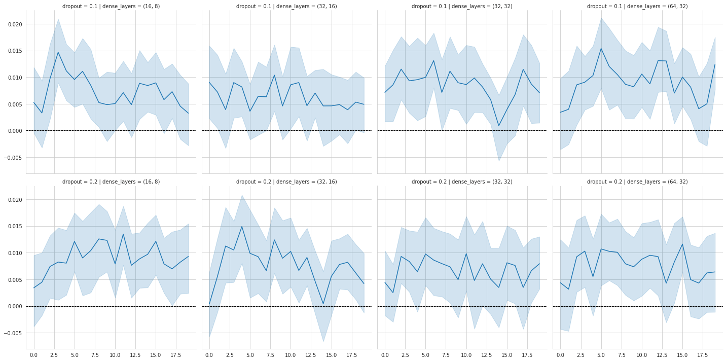
The purpose here is to visualize how model performance changes over training time for the different neural network settings that were tested. It takes the long-form results table, keeps only the runs with nonzero dropout, and then draws a line plot of IC against epoch. The figure is split into a grid so that each column corresponds to one dense-layer architecture and each row corresponds to one dropout level. That makes it easy to compare how the same training pattern behaves under different model sizes and regularization strengths.