


Deep Learning in Finance: LSTM Neural Networks for Stock Price Forecasting
Deep Learning in Finance: LSTM Neural Networks for Stock Price Forecasting
A LSTM Neural Network is used in this article to predict stock prices with the help of machine learning.

Machine learning is getting more important as Wall Street relies more and more on algorithms, with around 70% of orders being placed by software.
Keras will be used for building an LSTM model that predicts stock prices based on historical data, and we’ll show visualizations and optimal parameters. In this article, readers will learn what machine learning and LSTM networks can do for stock market predictions.
Get Data
import pandas as pd
import datetime

def get_historical_data(symbol,start_date,end_date):
    ''' Daily quotes from Google. Date format='yyyy-mm-dd' '''
    symbol = symbol.upper()
    start = datetime.date(int(start_date[0:4]), int(start_date[5:7]), int(start_date[8:10]))
    end = datetime.date(int(end_date[0:4]), int(end_date[5:7]), int(end_date[8:10]))
    url_string = "http://www.google.com/finance/historical?q={0}".format(symbol)
    url_string += "&startdate={0}&enddate={1}&num={0}&ei=KKltWZHCBNWPuQS9147YBw&output=csv".format(start.strftime('%b%d,%Y'), end.strftime('%b%d,%Y'),4000)

    col_names = ['Date','Open','High','Low','Close','Volume']
    stocks = pd.read_csv(url_string, header=0, names=col_names)

    df = pd.DataFrame(stocks)
    return df
Get historical stock quotes for a given symbol from Google Finance between two specified dates with this function called get_historical_data.
The function takes three parameters: symbol, start_date, and end_date. Symbol is a string representing the stock symbol, start_date represents the start date, and end_date represents the end date.
We convert the input symbol to uppercase letters inside the function. Then, we use the datetime module to convert the dates from strings to dates.
Next, a URL is constructed using the input symbol and the start and end dates, and the read_csv function from the pandas library is used to retrieve historical stock data. It’s a pandas DataFrame object with columns named ‘Date’, ‘Open’, ‘High’, ‘Low’, ‘Close’, and ‘Volume’.
The function returns the historical stock data in a DataFrame object.
Get the data from google.
data = get_historical_data('GOOGL','2005-01-01','2017-06-30') # from January 1, 2005 to June 30, 2017With the inputs ‘GOOGL’ (representing Alphabet Inc. — Class A’s stock symbol) as the symbol parameter, ‘2005–01–01’ as start_date, and ‘2017–06–30’ as end_date, this code calls the get_historical_data function.
From January 1, 2005, to June 30, 2017, this function gets historical GOOGL stock quotes from Google Finance. Assign the variable data to the pandas DataFrame object returned.
Write the data to a csv file
data.to_csv('google.csv',index = False)Using the to_csv method from the pandas library, this code writes DataFrame object data to a CSV file ‘google.csv’. By specifying index=False, you don’t want the index of the DataFrame included in the output.
This will create a CSV file with the same columns as the original DataFrame object data, with each row representing one day of historical GOOGL stock data between January 1, 2005, and June 30, 2017. You’ll save it to your current working directory.
Preprocess Data
import pandas as pd
import numpy as np

data = pd.read_csv('google.csv')
print(data.head())

print("\n")
print("Open   --- mean :", np.mean(data['Open']),  "  \t Std: ", np.std(data['Open']),  "  \t Max: ", np.max(data['Open']),  "  \t Min: ", np.min(data['Open']))
print("High   --- mean :", np.mean(data['High']),  "  \t Std: ", np.std(data['High']),  "  \t Max: ", np.max(data['High']),  "  \t Min: ", np.min(data['High']))
print("Low    --- mean :", np.mean(data['Low']),   "  \t Std: ", np.std(data['Low']),   "  \t Max: ", np.max(data['Low']),   "  \t Min: ", np.min(data['Low']))
print("Close  --- mean :", np.mean(data['Close']), "  \t Std: ", np.std(data['Close']), "  \t Max: ", np.max(data['Close']), "  \t Min: ", np.min(data['Close']))
print("Volume --- mean :", np.mean(data['Volume']),"  \t Std: ", np.std(data['Volume']),"  \t Max: ", np.max(data['Volume']),"  \t Min: ", np.min(data['Volume']))
DataFrame object is assigned to the variable data after reading the CSV file ‘google.csv’ with pandas’ read_csv function.
With numpy’s mean, standard deviation, maximum, and minimum functions, the code calculates and prints the mean, standard deviation, maximum, and minimum values of the ‘Open’, ‘High’, ‘Low’, ‘Close’, and ‘Volume’ columns.
A DataFrame’s head method prints the first five rows of the DataFrame to the console. The data from the CSV file is shown here in a brief preview.
Here’s a basic statistical summary of historical stock data for GOOGL, including price ranges and trading volumes, as well as central tendency and variability.
Remove Unecessary Data
import preprocess_data as ppd
stocks = ppd.remove_data(data)

#Print the dataframe head and tail
print(stocks.head())
print("---")
print(stocks.tail())
It looks like this code uses a custom module called preprocess_data that has a function called remove_data.
DataFrames have a remove_data function that removes any rows with missing or invalid data from the DataFrame. Stocks is then assigned the resulting DataFrame object.
Using the head and tail methods from the pandas library, the code prints the first five rows and last five rows of the stocks DataFrame. Seeing the cleaned data allows us to make sure it’s processed correctly.
In general, this code seems to be cleaning historical stock data for GOOGL so that it can be used for analysis or modeling later.
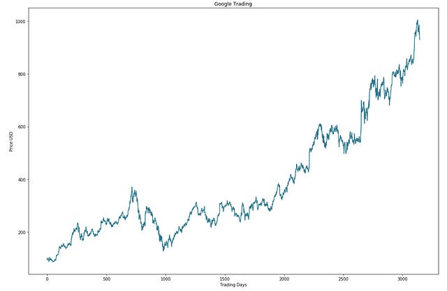
Visualise Raw Data
import visualize

visualize.plot_basic(stocks)
There’s a custom module called visualize in this code, which probably has functions for visualizing data.
In this code, the stocks DataFrame is passed into a function called plot_basic from the visualize module. To visualize the overall trend and outliers in the data, this function likely creates a basic plot of the stock data.
There’s no way to tell what the resulting plot will look like without knowing the exact details of plot_basic. GOOGL’s historical stock data is probably visualized with this code.
Normalise Data Using MinMax Scalar
stocks = ppd.get_normalised_data(stocks)
print(stocks.head())

print("\n")
print("Open   --- mean :", np.mean(stocks['Open']),  "  \t Std: ", np.std(stocks['Open']),  "  \t Max: ", np.max(stocks['Open']),  "  \t Min: ", np.min(stocks['Open']))
print("Close  --- mean :", np.mean(stocks['Close']), "  \t Std: ", np.std(stocks['Close']), "  \t Max: ", np.max(stocks['Close']), "  \t Min: ", np.min(stocks['Close']))
print("Volume --- mean :", np.mean(stocks['Volume']),"  \t Std: ", np.std(stocks['Volume']),"  \t Max: ", np.max(stocks['Volume']),"  \t Min: ", np.min(stocks['Volume']))
There’s a function called get_normalised_data in another custom module called preprocess_data.