Deep Learning Models: Calculating Precision, Recall, F1, and More
A test dataset must be used to evaluate the performance of your deep learning neural network model.

By reporting performance, you can both compare candidate models and communicate to stakeholders how well the model solves the problem.
Model performance can only be reported using limited metrics within Keras’ deep learning API model.
An example is provided to illustrate how metrics are calculated to evaluate a deep-learning neural network model.
You will know the following after completing this tutorial:
A guide to evaluating deep learning models using the scikit-learn metrics API.
With a final model required by scikit-learn API, you can make predictions about both classes and probability.
Here are some tips for calculating precision, recall, F1-score, ROC AUC, and more for a model by using the scikit-learn API.
Binary Classification Problem
Here, we will use the “two circles” problem as the basis for our binary classification tutorial.
When plotted, the problem consists of two concentric circles, one for each class, which is why it is known as the two circles problem. In this case, we are dealing with a binary classification problem. A graph can be drawn by interpreting the inputs as x and y coordinates. There are two circles: the inner circle and the outer circle.
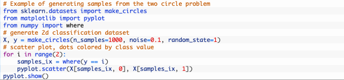
The make_circles() function in the scikit-learn library can be used to generate samples from the two circles problem. Each sample can be generated equally by specifying the number of samples. The “noise” argument increases the difficulty of classification by adding random statistical noise to the inputs or coordinates. The “random_state” argument specifies the seed for the random state The code generates the same samples every time, thanks to a pseudorandom number generator.
With 0.1 statistical noise and a seed of 1, the following example generates 1,000 samples.

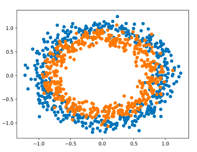
In order to understand how challenging the classification task is, we can plot the dataset once it is generated.
A sample plot is shown below, with colored points according to the class, with class 0 (the outer circle) colored blue and class 1 (the inner circle) colored orange.
In the example, the dataset is generated and plotted on a graph which clearly shows concentric circles for points in classes 0 and 1.
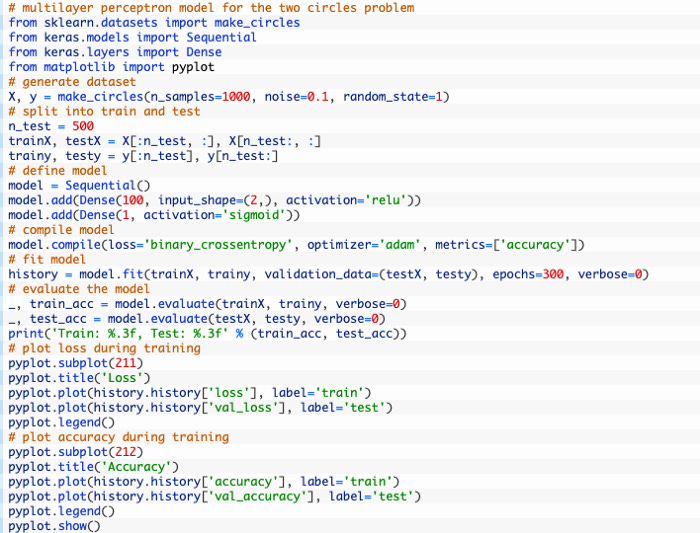
Multilayer Perceptron Model
In order to solve the binary classification problem, we will develop a Multilayer Perceptron model, or MLP.
Despite the fact that this model is not optimized for the problem, it is skillful (better than chance).
In order to train and evaluate the model, we will split the dataset into two equal parts.

Our MLP model can now be defined. Simple model, with 2 input variables from the dataset, a hidden layer with 100 nodes and a ReLU activation function, and an output layer with a single node and a sigmoid activation function.
Input examples will be classified as class 0 or class 1 based on the model’s prediction between 0 and 1.

The loss function for the model will be the binary cross entropy loss function, which will be fitted using the Adam version of stochastic gradient descent. Besides the classification accuracy metric, the model will also monitor it.

With the default batch size of 32 samples, we will fit the model for 300 training epochs and evaluate its performance at the end of each training epoch.

Our final model will be evaluated once more on the train and test datasets and the classification accuracy will be reported.

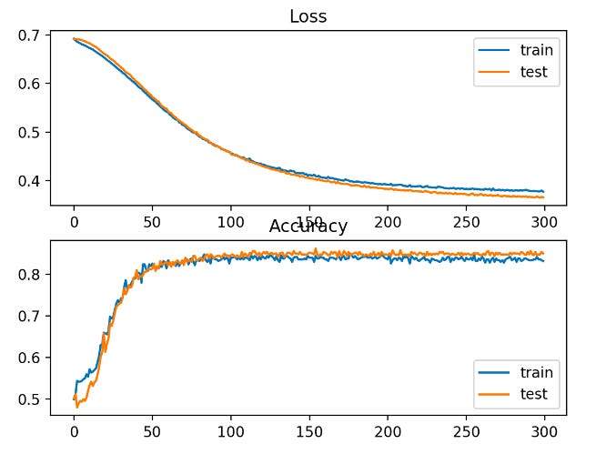
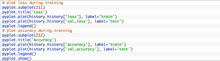
Lastly, a line plot will be used to show the loss and classification accuracy of the model on each of the train and test sets recorded during training.
In order to train and evaluate an MLP on the two circles problem, the following code listing is included.
When the example is run on the CPU, the model can be fitted very quickly (no GPU is required).
According to the evaluation, the model has a classification accuracy of 83% on train and 85% on test sets.

There are two line plots in the figure: one for the learning curves of the train and test sets suffered a loss and the train and test sets suffered a classification loss.
According to the plots, the model fits the problem well.