

Deep Learning Models for Predicting Stock Prices
For predicting numeric values and binary variables, machine learning uses linear regression.

In addition to nearest neighbors, support vector machines, decision trees, random forests, and boosting, you learn several other popular methods.
In addition to learning the common methods of sklearn, learning deep learning methods is another common next step. Keras is a popular library for building deep learning models. Assume that you are comfortable with Python and have some experience with deep learning and the sklearn library. There is no expectation of exposure to Keras.
As a result of deep learning, so many cases can now be predicted using these models. Most traditional classification and regression predictions can be made with deep learning models that do not have “fancy” layers.
Deep Learning with no “fancy” layers
In addition to their ability to predict a number of different targets, convolutional neural networks are becoming renowned for their ability to recognize images. Time-series data analyses can benefit greatly from Recurrent Neural Networks (RNNs) and Long-Short Term Memory (LSTM) models. In this article, we will focus on these last two methods — RNNs and LSTMs. By using the Keras library, these methods will be used for forecasting.
Data
Time-series data for several stocks is used for this post. Here, we are training a model on the stock market data from 2006 to 2016, then using that model to predict 2017 prices.
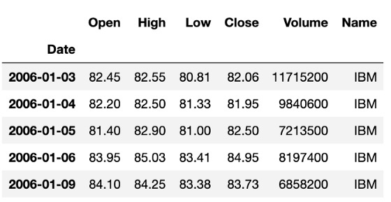
We have provided two examples below: Apple’s stock price and IBM’s stock price. We selected the High of the day for each of these plots. A blue line shows the training data and a red line shows the test data we are trying to predict.
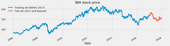
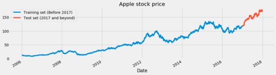
Apple and IBM stock prices are two examples of training and testing.
Models of traditional supervision versus models of recurrence
These machine learning algorithms use sklearn to predict values of y from columns of X, as described in the introduction.
For instance, Boston home prices can be predicted using this method. Data on housing is represented by X in this example. Y represents the price of the corresponding home. The X data is shown below:
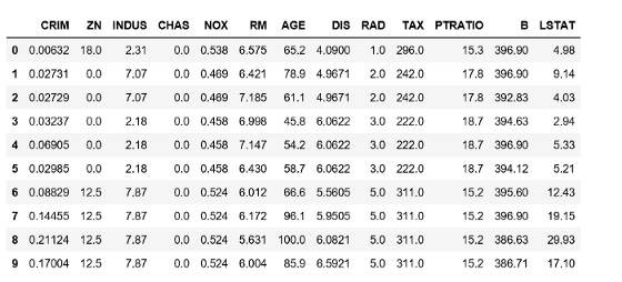
Home prices represent y for each row. Models are trained by connecting each row of X with the corresponding value of Y. It is not possible to have data that are all connected in this way when using time-series data. The trend from previous y values should be used instead to assist in predicting future y values.
You can see that each row represents a home in the Boston home price data. There is no connection between these homes. For time-series data, however, the price of the stock in the previous row is useful for predicting the price in the next row. Stock price relationships can be exploited using RNNs and LSTMs.
In A recurrent process can be implemented in Keras using SimpleRNN. LSTMs and GRUs.
Francois Chollet defines an RNN as a for loop that reuses values computed during previous iterations
Take advantage of these recurrent methods by putting them into practice.
Data Preprocessing
This recurrent network can only be used once we have preprocessed the data. In particular, we will examine the prediction of the High column. To set up this column for training and testing, follow these steps:
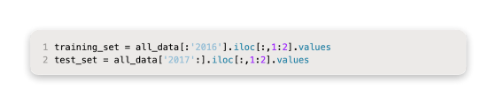
There are two types of training and test data: data from prior to 2017 (training) and data from after (test).
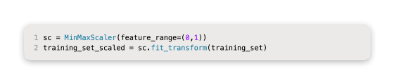
In order to scale this data, we do the following:
In order to predict the next day’s price, use the previous 60 days’ data. Here is a code snippet showing how to put this all together into a function:
RNNs, LSTMs, and GRUs
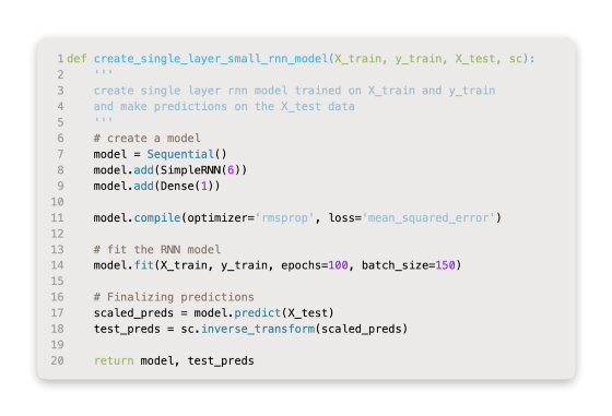
Now let’s go ahead and build a few recurrent models for predicting future stock prices by combining a few different functions. It might be a good idea to start with a super simple single-layer recurrent network with a very small number of nodes. An example of a single-layer, six-node model is shown below.
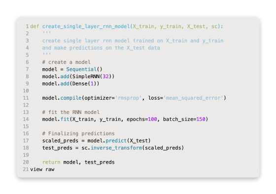
Adding more nodes to a model can often improve its performance. In order to improve a deep learning model, this is often the second step. Adding 32 nodes to the code below, we still have a single-layer model with additional nodes.
Multilayer recurrent models are commonly built to improve their prediction abilities by stacking several layers together. A model with fewer layers tends to underfit the data, while each layer preceding it tends to overfit the data.
A recurrent layer stack is a classic way to build more powerful recurrent networks. The Google Translate algorithm, for example, utilizes a stack of seven large LSTMs.” — Francois Chollet (Google Brain)
The example below shows how these recurrent layers can be stacked to create a model.
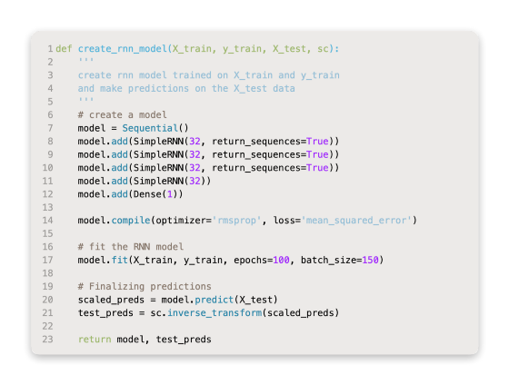
Stacking these layers of the network requires setting return_sequences=True in each layer leading up to the last recurrent layer. It is generally considered that the SimpleRNN model is useful only when it contains enough information to predict the next data point based on the most recent data point.
These multilayer models will usually outperform SimpleRNN layers because LSTM and GRU layers can take advantage of long-term dependencies by tackling what is called the vanishing gradient problem. By using these advanced layers, future predictions are more likely to be based on older information.
Although LSTM layers may slightly outperform GRU layers in practice, they generally achieve similar results. In general, however, GRU layers are preferred due to their lower computational cost. This example’s code can be found below.
