


Deep Reinforcement Learning on Stock Data
Deep Reinforcement Learning on Stock Data
Traditional analysis and decision-making methods have been used in financial trading for many years.

Artificial intelligence and machine learning have paved the way for innovative approaches such as Deep Reinforcement Learning (DRL), a powerful technique that blends deep learning and reinforcement learning.
This article examines DRL’s application to stock data analysis, demonstrating its transformative potential for financial trading. With DRL algorithms, investors can decipher hidden patterns, forecast market trends, and enhance trading strategies. Explore the intricacies of DRL and how it affects the stock market as we explore the future of finance accompanied by code snippets and charts.
Let’s start coding.
import time
import copy
import numpy as np
import pandas as pd
import chainer
import chainer.functions as F
import chainer.links as L
from plotly import tools
from plotly.graph_objs import *
from plotly.offline import init_notebook_mode, iplot, iplot_mpl
init_notebook_mode()
The code imports several Python modules and functions from those modules. The following is a line-by-line explanation:
The time module is imported, which provides time-related functions.
It imports the built-in copy module, which allows shallow and deep copies of objects to be created.
A Python module for numerical computations, numpy, is imported as np. For convenience, it is aliased as np.
This imports the third-party pandas module, a Python library for data manipulation and analysis. For convenience, it is aliased as pd.
Chainer is a Python deep learning framework imported from a third party.
For convenience, chainer.functions is imported and aliased as F.
Imports chainer.links as L: Aliases the links submodule from chainer as L.
Imports the tools module from the plotly library, a Python library for creating interactive data visualizations.
Imports all classes and functions from the plotly library’s graph_objs module. There are classes in this module that allow you to create various types of plots and charts.
Init_notebook_mode, iplot, and iplot_mpl are imported from plotly.offline: this imports the functions init_notebook_mode, iplot, and iplot_mpl. Plotly can be used in Jupyter notebooks with these functions, which enable interactive plotting without an internet connection.
The init_notebook_mode() function initializes the notebook mode of Plotly. Any Plotly function must be called before it can be used in a Jupyter notebook.
data = pd.read_csv('../input/Data/Stocks/goog.us.txt')
data['Date'] = pd.to_datetime(data['Date'])
data = data.set_index('Date')
print(data.index.min(), data.index.max())
data.head()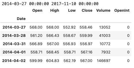
Using the pandas library in Python, this code loads stock data for Google from a CSV file and performs some basic data manipulation. In particular, it reads in a CSV file located at ‘../input/Data/Stocks/goog.us.txt’ and converts the ‘Date’ column into a pandas datetime object. The date column is then set as the index of the data DataFrame, which simplifies data manipulation. Using the min() and max() functions, the code prints the earliest and latest dates in the ‘Date’ column of the DataFrame. To verify that the data has been read in and manipulated correctly, the first five rows of the DataFrame are printed. The code can be used to quickly load and examine Google’s stock data, which can then be analyzed and modeled.
date_split = '2016-01-01'
train = data[:date_split]
test = data[date_split:]
len(train), len(test)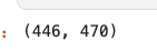
This Python code divides a dataset called ‘data’ into two parts, ‘train’ and ‘test’, based on the date ‘2016–01–01’. Datasets with a datetime index are assumed to be time-series data. Here is a line-by-line breakdown of the code:
date_split = ‘2016–01–01’:
In this line, the string ‘2016–01–01’ is assigned to a variable called date_split. The string represents a date, January 1st, 2016, which will be used as a reference point to split the dataset.
train = data[:date_split]:
It creates a new variable called train and assigns to it all rows of the dataset ‘data’ up to (but not including) the date specified by date_split. Therefore, it takes all the data with a date earlier than ‘2016–01–01’. Training will be done on this part of the dataset.
test = data[date_split:]:
A new variable called test is created and all the rows of the dataset ‘data’ are assigned to it from the date specified by date_split until the end of the dataset. This means that all data on or after ‘2016–01–01’ is taken into account. Testing will be conducted on this part of the dataset.
len(train), len(test):
Using this line, you can calculate the length (number of rows) of both the train and test datasets. Using this method, you can check the size of the two resulting datasets after splitting.
def plot_train_test(train, test, date_split):

    data = [
        Candlestick(x=train.index, open=train['Open'], high=train['High'], low=train['Low'], close=train['Close'], name='train'),
        Candlestick(x=test.index, open=test['Open'], high=test['High'], low=test['Low'], close=test['Close'], name='test')
    ]
    layout = {
         'shapes': [
             {'x0': date_split, 'x1': date_split, 'y0': 0, 'y1': 1, 'xref': 'x', 'yref': 'paper', 'line': {'color': 'rgb(0,0,0)', 'width': 1}}
         ],
        'annotations': [
            {'x': date_split, 'y': 1.0, 'xref': 'x', 'yref': 'paper', 'showarrow': False, 'xanchor': 'left', 'text': ' test data'},
            {'x': date_split, 'y': 1.0, 'xref': 'x', 'yref': 'paper', 'showarrow': False, 'xanchor': 'right', 'text': 'train data '}
        ]
    }
    figure = Figure(data=data, layout=layout)
    iplot(figure)
There are three arguments to the plot_train_test function in this code: train, test, and date_split. With the help of the Plotly library, this function creates an interactive plot that visualizes the train and test datasets as candlestick charts. Stock prices are represented by candlestick charts, which display four main price values: open, high, low, and close.
The function creates two candlestick traces (one for the train dataset and one for the test dataset) and combines them into one plot. In the date_split, the train dataset is displayed to the left, and the test dataset is displayed to the right. In the date_split, a vertical line separates the two datasets, and annotations indicate the train and test data regions.
The code is broken down into sections as follows:
Two Candlestick objects are created as part of the data variable, one for the train dataset and one for the test dataset. Candlestick objects are initialized with the dataset’s index (dates) and open, high, low, and close prices. To label the traces, the ‘name’ attribute is set to either ‘train’ or ‘test’.
As a dictionary, the layout variable contains ‘shapes’ and ‘annotations’. There is a single dictionary under the ‘shapes’ key that defines a vertical line at the date_split. At the top of the chart, adjacent to the vertical line, the ‘annotations’ key contains two dictionaries defining the text labels “train data” and “test data”.
The data and layout variables are used to create a Figure object. Candlestick traces and layout information are combined into a single Figure object.
A figure is passed as an argument to the Plotly library’s iplot() function. When the code is executed within a notebook or IDE, this function displays the interactive plot.
Essentially, this function creates an interactive candlestick chart to visualize and compare the train and test datasets separated by a vertical line.
plot_train_test(train, test, date_split)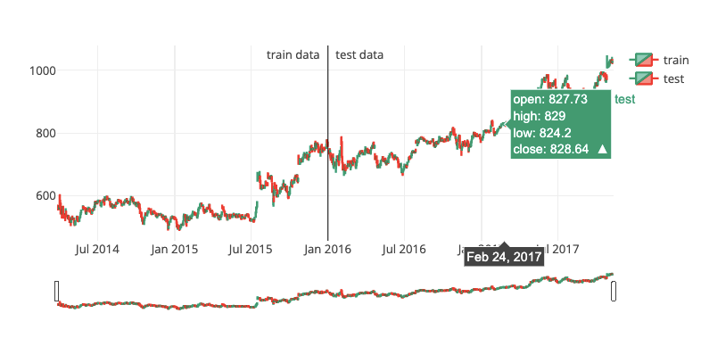
Three arguments are passed to the plot_train_test function: train, test, and date_split.
The training dataset is train, and the testing dataset is test. Reinforcement learning models are trained and evaluated using both datasets. The date_split variable specifies when the data is split into training and testing sets based on dates.
With plot_train_test, training and testing data are visualized as two separate time-series plots. The function generates a single plot containing two lines, one representing the training dataset and the other representing the testing dataset. This plot provides a visual representation of the data used for training and testing, allowing the user to examine the overall trends and distribution. It can also help identify discrepancies or unusual patterns between the training and testing datasets, which might affect the model’s performance.
class Environment1:

    def __init__(self, data, history_t=90):
        self.data = data
        self.history_t = history_t
        self.reset()

    def reset(self):
        self.t = 0
        self.done = False
        self.profits = 0
        self.positions = []
        self.position_value = 0
        self.history = [0 for _ in range(self.history_t)]
        return [self.position_value] + self.history # obs

    def step(self, act):
        reward = 0

        # act = 0: stay, 1: buy, 2: sell
        if act == 1:
            self.positions.append(self.data.iloc[self.t, :]['Close'])
        elif act == 2: # sell
            if len(self.positions) == 0:
                reward = -1
            else:
                profits = 0
                for p in self.positions:
                    profits += (self.data.iloc[self.t, :]['Close'] - p)
                reward += profits
                self.profits += profits
                self.positions = []

        # set next time
        self.t += 1
        self.position_value = 0
        for p in self.positions:
            self.position_value += (self.data.iloc[self.t, :]['Close'] - p)
        self.history.pop(0)
        self.history.append(self.data.iloc[self.t, :]['Close'] - self.data.iloc[(self.t-1), :]['Close'])

        # clipping reward
        if reward > 0:
            reward = 1
        elif reward < 0:
            reward = -1

        return [self.position_value] + self.history, reward, self.done # obs, reward, done
This code defines a Python class called Environment1, which represents a custom trading environment for reinforcement learning agents. It allows the agent to perform three actions: stay, buy, and sell based on time-series data of stock prices. Based on historical stock prices, the agent makes appropriate buy and sell decisions in order to maximize profits.
Here is a breakdown of the class and its methods:
__init__(self, data, history_t=90): This is the constructor method for Environment1. The agent takes two arguments: data, a DataFrame containing stock price data, and history_t, an optional parameter with a default value of 90, representing the number of historical data points it considers. In the constructor, input arguments are assigned to instance variables, and the reset() method is called to initialize the environment. Resets the environment to its initial state with reset(self).
This code sets the time step self.t to 0, the self.done flag to False (indicating that the environment is still running), and other variables related to the agent’s position and profits. Additionally, it creates a self.history list containing the specified number of zeros (based on self.history_t).
As a result of the method, an observation list is returned, which is a concatenation of the current self.position_value and the current self.history. In the environment, step(self, act) is called to perform one time step. A single argument, act, represents the agent’s action (0 for stay, 1 for buy, and 2 for sell). Based on the action taken, the method updates the agent’s positions, profits, and environment. Additionally, it calculates the reward the agent receives. A new position is added to self.positions at the current closing price if the agent decides to buy.
The agent’s reward is calculated based on the profits and losses from all open positions if the agent decides to sell. The agent receives a reward of -1 if there are no open positions. Positions and rewards remain unchanged if the agent stays. In addition to updating the agent’s positions and calculating the reward, the method updates the environment’s time step self.t, the agent’s position value, and the price history for the agent. Depending on whether the reward is negative, zero, or positive, it is clipped to -1, 0, or 1.
Lastly, the method returns an observation list (a concatenation of self.position_value and self.history), the calculated reward, and the self.done flag (which remains False because no termination condition exists in the environment). Essentially, this code defines a reinforcement learning trading environment class. Based on historical stock price data, the environment simulates a simplified trading scenario with three possible actions, allowing the agent to make buy and sell decisions accordingly.
env = Environment1(train)
print(env.reset())
for _ in range(3):
    pact = np.random.randint(3)
    print(env.step(pact))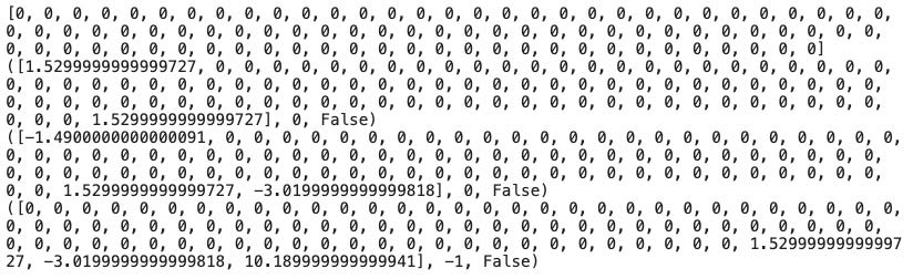
By taking random actions, the code creates an instance of the Environment1 class using the train dataset. By passing the train dataset as an argument, the Environment1 instance named env is created. The environment is then reset by calling the env.reset() method, which initializes the environment to its starting state and prints the initial observation.
A for loop is then used to perform three iterations, each representing one time step in the environment. Iteratively, a random action (pact) is generated using NumPy’s np.random.randint(3), which returns an integer between 0 and 2. Upon calling env.step(pact), the randomly generated action is updated in the environment, and the observation, reward, and ‘done’ flag are returned. Each time the agent takes a random action, these values are printed to show the outcomes.
This code snippet demonstrates how to create an instance of the custom trading environment Environment1 and interact with it by taking random actions. In this example, the environment’s reset() and step() methods are used to initialize and update the environment, respectively.
# DQNdef train_dqn(env): class Q_Network(chainer.Chain): def __init__(self, input_size, hidden_size, output_size):
super(Q_Network, self).__init__(
fc1 = L.Linear(input_size, hidden_size),
fc2 = L.Linear(hidden_size, hidden_size),
fc3 = L.Linear(hidden_size, output_size)
) def __call__(self, x):
h = F.relu(self.fc1(x))
h = F.relu(self.fc2(h))
y = self.fc3(h)
return y def reset(self):
self.zerograds() Q = Q_Network(input_size=env.history_t+1, hidden_size=100, output_size=3)
Q_ast = copy.deepcopy(Q)
optimizer = chainer.optimizers.Adam()
optimizer.setup(Q) epoch_num = 50
step_max = len(env.data)-1
memory_size = 200
batch_size = 20
epsilon = 1.0
epsilon_decrease = 1e-3
epsilon_min = 0.1
start_reduce_epsilon = 200
train_freq = 10
update_q_freq = 20
gamma = 0.97
show_log_freq = 5 memory = []
total_step = 0
total_rewards = []
total_losses = [] start = time.time()
for epoch in range(epoch_num): pobs = env.reset()
step = 0
done = False
total_reward = 0
total_loss = 0 while not done and step < step_max: # select act
pact = np.random.randint(3)
if np.random.rand() > epsilon:
pact = Q(np.array(pobs, dtype=np.float32).reshape(1, -1))
pact = np.argmax(pact.data) # act
obs, reward, done = env.step(pact) # add memory
memory.append((pobs, pact, reward, obs, done))
if len(memory) > memory_size:
memory.pop(0) # train or update q
if len(memory) == memory_size:
if total_step % train_freq == 0:
shuffled_memory = np.random.permutation(memory)
memory_idx = range(len(shuffled_memory))
for i in memory_idx[::batch_size]:
batch = np.array(shuffled_memory[i:i+batch_size])
b_pobs = np.array(batch[:, 0].tolist(), dtype=np.float32).reshape(batch_size, -1)
b_pact = np.array(batch[:, 1].tolist(), dtype=np.int32)
b_reward = np.array(batch[:, 2].tolist(), dtype=np.int32)
b_obs = np.array(batch[:, 3].tolist(), dtype=np.float32).reshape(batch_size, -1)
b_done = np.array(batch[:, 4].tolist(), dtype=np.bool) q = Q(b_pobs)
maxq = np.max(Q_ast(b_obs).data, axis=1)
target = copy.deepcopy(q.data)
for j in range(batch_size):
target[j, b_pact[j]] = b_reward[j]+gamma*maxq[j]*(not b_done[j])
Q.reset()
loss = F.mean_squared_error(q, target)
total_loss += loss.data
loss.backward()
optimizer.update() if total_step % update_q_freq == 0:
Q_ast = copy.deepcopy(Q) # epsilon
if epsilon > epsilon_min and total_step > start_reduce_epsilon:
epsilon -= epsilon_decrease # next step
total_reward += reward
pobs = obs
step += 1
total_step += 1 total_rewards.append(total_reward)
total_losses.append(total_loss) if (epoch+1) % show_log_freq == 0:
log_reward = sum(total_rewards[((epoch+1)-show_log_freq):])/show_log_freq
log_loss = sum(total_losses[((epoch+1)-show_log_freq):])/show_log_freq
elapsed_time = time.time()-start
print('\t'.join(map(str, [epoch+1, epsilon, total_step, log_reward, log_loss, elapsed_time])))
start = time.time()
return Q, total_losses, total_rewardsUsing the custom trading environment env, this code trains a Deep Q-Network (DQN). Q-Learning and deep neural networks are combined in DQN’s reinforcement learning algorithm. In this task, the goal is to learn a policy that maximizes the expected cumulative reward in the environment.
The code is broken down as follows:
Q_Network is defined as a subclass of Chainer’s chainer.Chain class. DQN’s neural network architecture is represented by it. There is a __init__ method in the class that initializes the network with three fully connected layers (L.Linear). __call__ defines the forward pass of the network using ReLU activation functions for the first two layers and linear output for the last layer. Resetting the gradients of the network is done using the reset method.
Train_dqn creates two instances of the Q_Network: Q and Q_ast. Q_ast is a copy of Q, which gets updated periodically, and Q is the main network.
There are a number of hyperparameters defined, including the number of epochs, the size of the replay memory, the batch size, the exploration rate (epsilon), the discount factor (gamma), and the frequency of network updates.
Iterating through the specified number of epochs is the main loop of the training process. In each epoch, the environment is reset, and an inner loop iterates. Every time step, the agent chooses an action either randomly (with probability epsilon) or by choosing the action with the highest Q-value predicted by the main network.
By using the env.step() method, the selected action is then executed in the environment. Replay memory stores the observation, reward, and ‘done’ flag. When the memory is full, old experiences are removed.
Training begins when the memory is full. Training frequency determines how often the network is trained. In mini-batches, the experiences in the memory are shuffled and the training is performed. Q_ast is used to calculate the target Q-values. After that, the main network Q is updated by minimizing the mean squared error between its predictions and the target Q-values.
Weights from the main network Q are periodically updated in the target network Q_ast. Over time, exploration rate epsilon decreases until it reaches a minimum.
Until all epochs have been completed, the training process continues. Periodically, the total rewards and losses are logged and printed.
The code defines a function that trains a DQN agent using a custom trading environment. Based on the experiences stored in the replay memory, the agent learns a trading policy by interacting with the environment.
Q, total_losses, total_rewards = train_dqn(Environment1(train))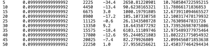
A custom trading environment Environment1 created with the train dataset is passed as an argument to the train_dqn() function. During the training process, the train_dqn() function returns three values: the trained Deep Q-Network (DQN) model Q, the total losses total_losses, and the total rewards total_rewards. In this line of code, these returned values are assigned to variables, which can be used for analyzing the performance of the trained DQN agent or making predictions.
def plot_loss_reward(total_losses, total_rewards): figure = tools.make_subplots(rows=1, cols=2, subplot_titles=('loss', 'reward'), print_grid=False)
figure.append_trace(Scatter(y=total_losses, mode='lines', line=dict(color='skyblue')), 1, 1)
figure.append_trace(Scatter(y=total_rewards, mode='lines', line=dict(color='orange')), 1, 2)
figure['layout']['xaxis1'].update(title='epoch')
figure['layout']['xaxis2'].update(title='epoch')
figure['layout'].update(height=400, width=900, showlegend=False)
iplot(figure)The code defines a function called plot_loss_reward, which takes two arguments: total_losses and total_rewards. As a result of the training process of a DQN agent, these represent the losses and rewards obtained. Using Plotly, a popular Python graphing library, this function creates a visual representation of these losses and rewards.