

Developer’s Guide to Bond Pricing Ep 4/365
Understanding Time Value of Money, Duration, and Convexity through Python.

Download source code and dataset using the button at the end of this article!
Bond valuation and selection are useful for rounding out your portfolio, primarily by determining a bond’s fair value based on its future cash flows and the time value of money.
This article examines the fundamental principles of bond valuation and how to assess a bond’s intrinsic value by calculating the present value of its future cash flows and its annual rate of return.
With these concepts in hand, you will be better equipped to make informed decisions about bond investments and portfolio construction.
import os
import sys
import subprocess
import warnings
import pandas as pd
import numpy as np

warnings.filterwarnings(”ignore”)

INSTALL_DEPS = False
if INSTALL_DEPS:
    subprocess.check_call([sys.executable, “-m”, “pip”, “install”, “numpy==1.23.4”])
    subprocess.check_call([sys.executable, “-m”, “pip”, “install”, “pandas==2.2.0”])
    IN_KAGGLE = IN_COLAB = False

try:
    import google.colab
    from google.colab import drive

    drive.mount(”/content/drive”)
    DATA_PATH = “/content/drive/MyDrive/fixedincome_dataset”
    IN_COLAB = True
    print(”Colab!”)
except Exception:
    IN_COLAB = False

if “KAGGLE_KERNEL_RUN_TYPE” in os.environ and not IN_COLAB:
    print(”Running in Kaggle...”)
    for dirpath, _, filenames in os.walk(”/kaggle/input”):
        for fname in filenames:
            print(os.path.join(dirpath, fname))
    DATA_PATH = “/kaggle/input/fixedincome-dataset”
    IN_KAGGLE = True
    print(”Kaggle!”)
elif not IN_COLAB:
    IN_KAGGLE = False
    DATA_PATH = “./data/fixed”
    print(”running localhost!”)
This code block’s responsibility is to detect which runtime environment the notebook or script is executing in, configure a consistent dataset path for downstream data loading, and optionally ensure reproducible dependency versions. At the top, warnings.filterwarnings(“ignore”) silences library warnings so notebook output stays clean during iterative quant research; this keeps experiment logs focused on results rather than transient library chatter.
The INSTALL_DEPS flag provides an opt-in mechanism to force-install specific numpy and pandas versions. If that flag is set true, the script runs pip to install pinned versions and then explicitly sets IN_KAGGLE and IN_COLAB to False; this branch is intended to create a reproducible library environment before any environment-specific mounting or path resolution happens. When INSTALL_DEPS is false (the default here), the script skips package installation and proceeds to environment detection.
Environment detection is performed in a two-stage, priority-driven way. First, the code attempts to import google.colab and mount a Google Drive. If that import succeeds, drive.mount(“/content/drive”) is called and DATA_PATH is set to “/content/drive/MyDrive/fixedincome_dataset”, and IN_COLAB is marked True. This sequence both authenticates access to persistent storage and establishes the dataset location for Colab runs, so subsequent data-loading code can rely on DATA_PATH to find the fixed-income dataset in the user’s Drive. The try/except ensures that a failed import (i.e., not running in Colab) does not crash the script but instead causes IN_COLAB to remain False.
After the Colab attempt, the code checks for a Kaggle environment by looking for the “KAGGLE_KERNEL_RUN_TYPE” environment variable, but only if we are not already in Colab. If that variable exists, it prints a short message, walks the /kaggle/input directory to list all files (which provides quick visibility into what datasets are present in the Kaggle session), sets DATA_PATH to “/kaggle/input/fixedincome-dataset”, and marks IN_KAGGLE True. That path choice makes the dataset available to later data-loading steps that expect the fixed-income files to live under Kaggle’s input directory.
If neither Colab nor Kaggle was detected, the code falls back to a local development assumption: it sets IN_KAGGLE False and DATA_PATH to a relative “./data/fixed” path and prints “running localhost!”. This provides a consistent, local default location for the same fixed-income dataset so the rest of the quant trading pipeline can operate unchanged regardless of the runtime. Throughout, simple print statements act as lightweight runtime logs indicating which branch was taken and confirming the DATA_PATH that downstream code should use.
Treasuries and the Composition of a T-Bill
U.S. Treasuries (T-Bills, T-Notes, T-Bonds) are the safest fixed-income instruments available, primarily because the U.S. government cannot default and can raise taxes to meet its obligations.
The 3-month T-Bill serves as the benchmark for the risk-free rate across portfolios; at the time of writing it is between 4.5% and 5.2%. A T-Bill is a zero-coupon fixed-income instrument: it pays no periodic interest and is sold at a discount to its face value.
T-Bills are straightforward. T-Notes resemble the typical bonds issued by other borrowers, with interest paid periodically.
From our dataset, let’s look at the attributes of a T-Note:
import pandas as pd

df_treasuries = pd.read_csv(f”{DATA_PATH}/treas1.csv”)
df_treasuries = df_treasuries.loc[:, df_treasuries.notna().any()]
df_treasuries.head(3)
The block begins by loading the raw treasury dataset from disk into a pandas DataFrame. The intent is to bring the on-disk CSV into an in-memory tabular structure so downstream quant models and computations can operate on it. The DATA_PATH variable determines the file location, which keeps file organization separate from the reading logic.
Next, the code filters out any columns that contain only missing values. It does this by building a boolean mask from df_treasuries.notna().any(): notna() produces a True/False matrix indicating which cells are present, and any() collapses that per column to True if at least one non-NA value exists. Using .loc[:, mask] selects all rows but only the columns for which that mask is True, so any column composed entirely of NaNs is dropped. This step ensures that subsequent numeric operations, statistical summaries, or feature engineering used for pricing, yield curve construction, or risk calculations are not polluted by entirely empty fields that would otherwise contribute no information.
Finally, df_treasuries.head(3) retrieves the first three rows of the cleaned DataFrame for a quick inspection. This call does not mutate the DataFrame; it simply returns a small sample view so the developer can confirm the top-level structure, column selection, and basic values before continuing into the quant pipeline where these treasury time series will be used for modeling, calibration, or signal generation.
Present Value of Money
The present value represents how much a future amount of money is worth today after adjusting for interest or discounting. Money received in the future is worth less than the same amount received today because it could be invested and earn a return. To find the intrinsic value of a T-Bill, the future payment is discounted back to the present using an appropriate rate.
The present value formula is shown below, centered for clarity.
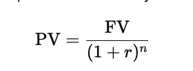
In this expression, PV stands for the value today, FV is the amount that will be received in the future, r is the interest or discount rate per period, and n is the number of time periods until payment. The larger the rate or the longer the time, the smaller the present value becomes because the future cash flow is discounted more heavily.
Discounting is the process of moving from the future back to the present. The opposite operation is compounding, which moves money from the present to the future. Rearranging the present value formula gives the future value formula shown below.
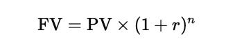
This second equation shows how a current amount grows over time when interest is applied repeatedly across periods.
face_value = 100
rate_percent = 4.165
period_rate = rate_percent / 100 / 2
periods = (2029 - 2023) * 2
present_value = face_value / pow(1 + period_rate, periods)
present_value
This code computes the present value of a bond’s redemption amount by applying a semiannual discounting model and expresses that calculation in a few explicit steps useful in quant trading for fixed-income valuation and relative-value analysis.
First, face_value = 100 defines the maturity principal (the cash that will be received at bond maturity). rate_percent = 4.165 holds the annual interest rate in percentage terms; the code immediately converts that into a per-period decimal by dividing by 100 to get a decimal fraction and then dividing by 2 to get the semiannual rate. That second division reflects the choice of semiannual compounding, which is the standard convention for many bonds: period_rate = rate_percent / 100 / 2.
Next, periods = (2029–2023) * 2 computes the total number of semiannual periods between the valuation date (implicitly 2023) and maturity in 2029. Subtracting the years gives the number of years to maturity (6), and multiplying by 2 converts years to semiannual periods, producing the exponent used in compounding/discounting (12 periods in this case).
Finally, present_value = face_value / pow(1 + period_rate, periods) applies the standard discounting formula PV = FV / (1 + r)^n to bring the future principal back to today. pow(1 + period_rate, periods) calculates the compounding factor for the entire remaining life, and dividing the face value by that factor yields its present value under semiannual compounding at the given annual rate. In the context of quant trading, this is a basic instrument-pricing step: it produces the present value of the redemption cash flow using the specified discount rate and compounding convention, a building block for pricing, yield calculations, and portfolio mark-to-market for fixed-income instruments.
A discrepancy exists between the T-Bill’s price (Ask) and its present value (PV). To properly evaluate the bond, we use other formulas.
Bond Valuation
A bond’s value today is equal to the present value of all coupon payments it will make in the future, together with the present value of the final face value (principal) that is repaid at maturity. Each of these cash flows is discounted back to the present because future money is worth less than money today.
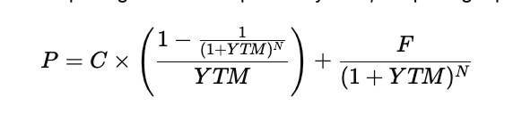
The general bond valuation formula is:
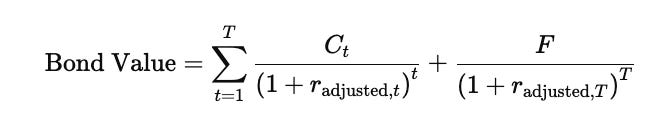
The first term represents the sequence of coupon payments discounted back to the present, while the second term represents the present value of the face value that is received at maturity.
When the coupon payment is the same every period and the discount rate is also constant, the stream of coupons forms an annuity. In that special case, the present value of the coupon payments can be written in a much simpler closed form as:
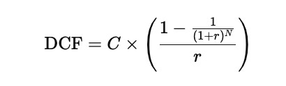
In this simplified setting, C is the constant coupon payment in each period, r is the constant discount rate, and N is the total number of periods until maturity. The face value is still discounted separately using the same rate over N periods, and then added to the discounted coupon value to obtain the total bond price.
The discount rate used in practice is often the yield to maturity, although it may also be adjusted to account for taxes, inflation, or other risk considerations depending on the context.
This framework is the foundation of bond pricing, and financial calculators or programming tools can evaluate these expressions directly once the cash flows, discount rate, and maturity are known.
coupon = 3.875 / 2
par = 100
semi_rate = 4.165 / 100 / 2
num_periods = (2029 - 2023) * 2

pv_coupons = sum(coupon / (1 + semi_rate) ** t for t in range(1, num_periods + 1))
pv_par = par / (1 + semi_rate) ** num_periods

present_value = pv_coupons + pv_par
print(present_value)
This block computes the present value (price) of a fixed-rate bond that pays semiannual coupons, using a quoted annual yield converted to the matching semiannual periodic rate. The overall goal is to take the bond’s scheduled cash flows (semiannual coupon payments plus a single principal repayment at maturity) and discount each one to today’s value so the result is a mark-to-market price per 100 of par — a routine building block in quant trading for valuation, P&L, spread analysis, and relative-value comparisons.
coupon = 3.875 / 2 establishes the cash amount paid each semiannual period. The 3.875 is an annual coupon rate expressed on a 100 par basis (i.e., 3.875% of par = 3.875 units per year). Dividing by 2 converts that annual coupon into the actual payment amount received every six months (so you get the per-period cash flow consistent with semiannual payments).
par = 100 sets the notional principal against which coupon percentages are applied; pricing here is therefore expressed as a value per 100 of face. semi_rate = 4.165 / 100 / 2 converts the quoted annual yield of 4.165% into the periodic yield per semiannual period: first dividing by 100 to convert percentage to a decimal, then dividing by 2 to reflect semiannual compounding. Aligning the yield’s compounding frequency with the coupon payment frequency is the key reason for this conversion — using mismatched frequencies would mis-discount the cash flows.
num_periods = (2029–2023) * 2 computes how many semiannual cash flows remain until maturity. By taking the year difference and multiplying by 2, the code turns remaining years into the count of six-month periods; this count drives both the loop that discounts coupons and the timing of the principal repayment.
pv_coupons = sum(coupon / (1 + semi_rate) ** t for t in range(1, num_periods + 1)) iterates over each future coupon payment and discounts it back to present value using the standard discrete compounding discount factor (1 + periodic_rate)^t. Conceptually this is the present value of an annuity of fixed payments: each coupon amount is divided by the appropriate compound factor based on how many periods until that payment. pv_par = par / (1 + semi_rate) ** num_periods applies the same discounting to the single principal repayment at maturity, placing that cash flow at the final period.
present_value = pv_coupons + pv_par then aggregates the discounted coupon stream and the discounted principal into the bond’s total present value (the clean price per 100 par as computed here). Printing that value yields the numeric price used in downstream quant workflows — for example, to compare against market quotes, compute yield spreads, or incorporate into portfolio valuations and risk calculations.
The price of 98.47 is closer to the ask price of 98.60. Because this is a market, prices are not always perfectly fair. Yield to maturity (YTM) is the primary driver of price; for this T-Bill the ask yield is 4.165%.
Yield to Maturity (YTM)
Yield to maturity is the single discount rate that makes the present value of all future coupon payments and the face value exactly equal to the current market price of the bond. In other words, it is the internal rate of return earned by an investor who buys the bond at today’s price and holds it until maturity, assuming all coupons are reinvested at the same rate.
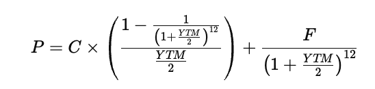
If the discount rate in the bond pricing formula is replaced by YTM, the pricing equation becomes
This equation is nonlinear because the unknown YTM appears both in the denominator and inside the exponent. For that reason there is no simple algebraic rearrangement that isolates YTM on one side. Instead, it must be solved numerically. Financial calculators and spreadsheet functions do this automatically, but the same result can be obtained using iterative root-finding methods such as Newton–Raphson.
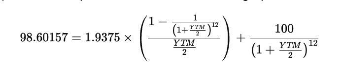
For the Treasury note described, the annual coupon rate is 3.875 percent on a face value of 100, with semi-annual payments from January 2023 until December 2029, which gives twelve total coupon periods. Semi-annual payments mean the annual coupon and the yield are both divided by two when expressed per period. Substituting semi-annual compounding into the pricing relationship produces
With the numerical values substituted, the unknown variable is only YTM, because the price, coupon per period, face value, and number of periods are all known. The resulting equation is
To solve this, define a function that measures the difference between the left and right sides of the equation. The goal is to find the YTM that makes this difference equal to zero. That function can be written as
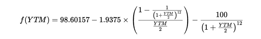
The Newton–Raphson method starts from an initial guess for YTM and repeatedly improves that guess by subtracting the function value divided by its derivative. The general update rule is
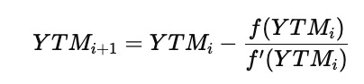
The derivative f′(YTM) is obtained by differentiating the pricing expression with respect to YTM, which captures how the price changes when the yield changes. By repeatedly applying the update formula, the successive estimates move closer to the true yield. The process stops when two consecutive estimates are almost the same, meaning the method has converged.
In practice, only a few iterations are usually required, and the final value produced is the bond’s yield to maturity consistent with the observed market price.
import numpy as np

market_price = 98.60157
coupon_per_period = 3.875 / 2
par_value = 100.0
total_periods = 12

def price_difference(y):
    r = y / 2
    df = 1 + r
    annuity = coupon_per_period * ((1 - df**(-total_periods)) / r)
    redemption = par_value / df**total_periods
    return market_price - (annuity + redemption)

def derivative_price(y):
    r = y / 2
    df = 1 + r
    a = (coupon_per_period / 2) * (total_periods / df**(total_periods + 1))
    b = coupon_per_period * ((1 - df**(-total_periods)) / r**2)
    c = (par_value * total_periods) / (2 * df**(total_periods + 1))
    return - (a - b + c)

def newton_solver(start, tol=1e-5, max_iter=20):
    x = start
    for _ in range(max_iter):
        next_x = x - price_difference(x) / derivative_price(x)
        if np.abs(next_x - x) < tol:
            return next_x
        x = next_x
    return x

initial_guess = 0.04
given_ytm = 0.04165
computed_ytm = newton_solver(initial_guess)
print(f”Calculated: {computed_ytm} vs stated: {given_ytm}”)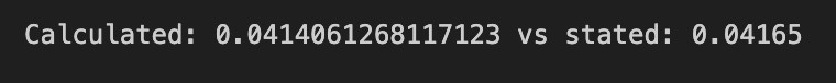
This module is solving for a bond’s yield-to-maturity (YTM) by finding the interest rate y that makes the present value of the bond’s cash flows equal to its market price. The top-level parameters set the fixed inputs: market_price is the observed price you want to match, coupon_per_period divides the annual coupon by 2 because coupons are paid semiannually, par_value is the face value paid at maturity, and total_periods is the number of semiannual periods remaining. Using semiannual periods is why the code consistently halves y (treating y as an annual nominal rate convertible semiannually) and uses df = 1 + r as the per-period discount factor.
The price_difference function computes market_price minus the present value of the bond cash flows at a candidate yield y. It first maps the annual nominal yield y to the per-period rate r = y/2 and forms the per-period discount factor df = 1 + r. It then computes the annuity term as the present value of all remaining coupon payments using the standard finite-geometric sum formula: coupon_per_period * ((1 — df**(-total_periods)) / r). Redemption is the present value of par at maturity, par_value / df**total_periods. The function returns market_price — (annuity + redemption); the root of this function (where it equals zero) is the YTM that prices the bond to the observed market price.
The derivative_price function implements the derivative of that price difference with respect to the annual yield y, which Newton’s method needs as the denominator of the correction step. Internally it reuses r = y/2 and df = 1 + r. It then computes three algebraic components that arise when differentiating the annuity and redemption terms with respect to y using the chain rule (accounting for dr/dy = 1/2 and d(df)/dy = 1/2): a represents a term coming from differentiating the df**(-N) structure that appears inside the annuity, b corresponds to the contribution from differentiating the 1/r factor in the annuity expression (the r**-2 structure), and c corresponds to differentiating the redemption (par value times df**(-N)). The function returns — (a — b + c), which aligns with taking the derivative of market_price — PV(y) (market_price is constant so its derivative is zero) and therefore supplies the slope of the price-difference function at the current y.
The newton_solver function applies Newton–Raphson iteration to find the root of price_difference. It begins from a supplied start value for y, then iteratively computes the Newton update next_x = x — price_difference(x) / derivative_price(x). After each update it checks the absolute change |next_x — x| against a tolerance tol; if the change is smaller, it considers the estimate converged and returns the current root estimate. If convergence is not reached within max_iter iterations it returns the last iterate. This use of Newton’s method is standard for root finding in quant finance because it typically converges rapidly near the root when a reasonable derivative is available.
Finally, the script supplies an initial guess of 0.04 (4% annual), calls newton_solver to compute the YTM that prices the bond to market_price, and prints the calculated result alongside a stated YTM (given_ytm) for comparison. In the context of quantitative trading, this sequence is directly about converting an observed bond price into an implied yield, a fundamental step for mark-to-market, relative value calculations, curve construction, and any strategy that depends on consistent yield measures across instruments.
Two additional attributes that sophisticated bond investors consider are duration and convexity.
Duration
Duration measures a bond’s price sensitivity to changes in market interest rates. When interest rates rise, bond prices fall because newly issued instruments offer higher yields; when rates fall, bond prices rise.
Convexity
Convexity describes how a bond’s price sensitivity (duration) changes as yields change — in other words, it captures the curvature of the price–yield relationship. Practically, yields increase as prices fall; if market interest rates exceed a bond’s coupon, the bond’s price must decline to raise its yield to market levels.
Interest-rate risk
Duration and convexity are the primary tools used to manage interest-rate risk. For our purposes — purchasing bonds with the intention of holding them to maturity — we accept interest-rate risk.
Credit (default) risk
One risk we will not accept is default risk. U.S. Treasuries are generally treated as risk-free; many other bonds (particularly private-sector issues) carry default risk. When selecting bonds, choose investment-grade ratings from Moody’s or S&P — generally A-range and above, with AAA being the highest.
High-yield and call (recall) risk
Bonds with elevated default risk offer higher yields to compensate investors; these are commonly referred to as high-yield or “junk” bonds (see, for example, sovereign defaults such as Argentina in 2001). Another risk to avoid is call (recall) risk: some bonds can be called and refinanced when interest rates fall. If an issuer calls a bond, holders receive the face value and must reinvest proceeds, typically at lower prevailing yields.
Ranking our Fixed Income Dataset
We load our dataset, which comprises Treasuries, municipals (munis), corporate bonds, and certificates of deposit (CDs). These instruments can be retrieved from a broker’s bond scanner:
import os
import pandas as pd

def _read_and_tag(csv_path, tag):
    df = pd.read_csv(csv_path)
    df[’Instrument Type’] = tag
    df[’Ask’] = pd.to_numeric(df[’Ask’], errors=’coerce’)
    df[’Coupon’] = pd.to_numeric(df[’Coupon’], errors=’coerce’)
    df.fillna(0, inplace=True)
    return df

def collect_fixedinc_files():
    PREFIX_TO_LABEL = {
        ‘cds’: ‘Certificates of Deposit’,
        ‘corp’: ‘Corporate Bonds’,
        ‘munies’: ‘Municipal Bonds’,
        ‘treas’: ‘Treasuries’
    }

    frames = []
    for fname in os.listdir(DATA_PATH):
        if not fname.endswith(’.csv’):
            continue
        path = os.path.join(DATA_PATH, fname)
        for prefix, label in PREFIX_TO_LABEL.items():
            if fname.startswith(prefix):
                frames.append(_read_and_tag(path, label))
    if frames:
        return pd.concat(frames, ignore_index=True)
    return pd.DataFrame()

fixedinc_data = collect_fixedinc_files()
fixedinc_data.dropna(axis=1, how=’all’, inplace=True)
fixedinc_data.dropna(axis=0, inplace=True)

fixedinc_data = fixedinc_data[fixedinc_data[’Ask’] > 0]
fixedinc_data[’Ask Yield’] = pd.to_numeric(fixedinc_data[’Ask Yield’], errors=’coerce’)
fixedinc_data = fixedinc_data[fixedinc_data[’Ask Yield’] > 0]

fixedinc_data.tail(2)
The code builds a single, analysis-ready table of fixed-income instruments by discovering CSV files, labeling each row with an instrument type, normalizing key numeric fields, and filtering out records that are unusable for pricing and analytics.
First, _read_and_tag(csv_path, tag) loads one CSV into a DataFrame and immediately attaches a semantic label in a new column, “Instrument Type”, so downstream logic can group or filter by security class (e.g., treasuries vs corporates). It explicitly coerces the Ask and Coupon columns to numeric types (non-numeric strings become NaN) so those fields are guaranteed to be numeric for later computations. After the coercion it calls fillna(0), replacing any remaining missing values with zeros inside that per-file frame; this ensures the file-level DataFrame has no nulls in places the code expects numeric defaults and prevents simple downstream operations from failing due to missing entries.
collect_fixedinc_files() drives file discovery and aggregation. It defines a prefix→label mapping so only files whose names begin with known fixed-income prefixes are treated as relevant market feeds. The function iterates DATA_PATH, ignores non-CSV files, and for each CSV whose filename starts with a recognized prefix it calls _read_and_tag with the mapped human-readable instrument label, collecting each returned frame into a list. If at least one matching file was found the list of frames is concatenated into a single DataFrame with reset indexing (ignore_index=True) to produce a unified dataset; if none are found an empty DataFrame is returned. This consolidates multiple per-issue or per-instrument CSVs into one canonical table keyed by instrument type.
After aggregation, the script performs a sequence of cleaning and validation steps to leave only rows suitable for quant workflows. It first drops any columns that are entirely empty (dropna axis=1 how=’all’), removing unused metadata columns that convey no information. Then it drops any rows containing NaNs (dropna axis=0), eliminating partially populated records that could corrupt numeric analyses. Next it filters the rows to only those where Ask > 0; this enforces that only instruments with a positive market ask price remain, which is necessary for any pricing, risk, or trade sizing logic. The code then coerces the “Ask Yield” column to numeric (errors become NaN) and filters again for Ask Yield > 0, ensuring the dataset includes only instruments with valid, positive yields that can feed yield-curve models, spread computations, and return calculations.
Finally, fixedinc_data.tail(2) produces the last two rows of the resulting DataFrame for inspection. In the context of quant trading, this pipeline produces a labeled, numeric, and filtered universe of fixed-income instrument records ready for modeling steps such as yield curve fitting, spread analysis, or trade signal generation.
We set the constants for the market regime as of the time of writing:
COMMISSION = 1  # Average $1 commissions
TAX = 0.30
AFTER_TAX_RF = 0.0375 * (1 - TAX)
CPI = 0.025
PAR = 100.0

REAL_DISCOUNT = (1.0 + AFTER_TAX_RF) / (1.0 + CPI) - 1.0
REAL_DISCOUNT
This block defines a small set of constants and computes an inflation-adjusted, after‑tax discount rate that you can use when valuing cash flows or benchmarking strategy returns in a quant trading context. The intent is to convert a nominal, after‑tax risk‑free return into a real rate that removes the erosion from expected inflation, so downstream pricing and performance comparisons are on an apples‑to‑apples, inflation‑adjusted basis.
First, COMMISSION is set to 1, representing a fixed average commission of $1 per trade; TAX is set to 0.30 to represent a 30% tax rate. Those two constants parametrise transaction and tax assumptions that affect net returns and cost calculations elsewhere in the strategy (commissions reduce net P&L; the tax rate is used to convert nominal yields into after‑tax yields). AFTER_TAX_RF is computed next as 0.0375 * (1 — TAX): the hardcoded 0.0375 is the nominal risk‑free rate (3.75%), and multiplying by (1 − TAX) reduces that nominal yield to the after‑tax nominal yield (here 0.0375 * 0.7 = 0.02625, i.e., 2.625%). This models the fact that interest‑type returns are subject to taxation, so the cash available for reinvestment or consumption is lower than the headline nominal rate.
CPI is set to 0.025 to represent expected inflation of 2.5%, and PAR is set to 100.0 as a conventional face value used for bond or fixed‑income calculations (par isn’t used in the subsequent computation here but is declared for pricing or yield conversions elsewhere). REAL_DISCOUNT is then calculated as (1.0 + AFTER_TAX_RF) / (1.0 + CPI) — 1.0. This implements the standard Fisher adjustment to convert a nominal after‑tax rate into a real rate: you divide the gross after‑tax return (1 + nominal_after_tax) by the gross inflation factor (1 + CPI) and subtract 1 to get the real, inflation‑adjusted rate. Numerically this yields (1.02625 / 1.025) − 1 ≈ 0.0012195, or about 0.122% real, after‑tax.
In quant trading terms, that REAL_DISCOUNT is the real hurdle or discount rate you would apply when discounting expected future cash flows, comparing strategy returns net of tax and inflation, or assessing whether a trade’s expected excess return justifies execution costs (like the COMMISSION). The calculation ensures that comparisons and valuations reflect the true purchasing‑power return available after taxes and inflation have been accounted for.
Earlier we noted that the yield to maturity (YTM) can serve as a discount rate; however, that is a market-derived measure from the secondary market, and we may prefer to use a custom discount rate.
Assume the risk-free rate equals the average yield on a DGS‑insured European savings account: 3.75% nominal, with interest taxed at 30%. We will not use the 10‑year T‑bill as a proxy because doing so would require adjustments for secondary‑market yields and commissions. The risk‑free (RF) rate here represents the opportunity cost of investing in a riskier bond; inflation is approximately 2.5%.
Using this information, we construct our own discount rate — specifically the real rate adjusted for inflation and taxation.
The Fisher Equation for Real Interest Rates
The Fisher equation connects the nominal interest rate, the real interest rate, and the inflation rate through compounding rather than simple subtraction. It recognizes that inflation erodes purchasing power, so the real rate reflects the true increase in purchasing power earned on an investment.
The compounded Fisher relationship is

This states that the growth of money in nominal terms is equal to the combined effect of real growth and inflation together. Rearranging this equation to isolate the real interest rate gives
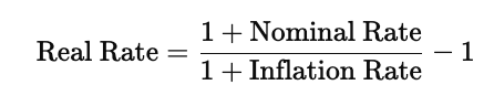
This version shows directly how the real rate is obtained by adjusting the nominal rate for inflation. When inflation is low, an approximate rule often used in practice is that the real rate is roughly equal to the nominal rate minus inflation, but the exact Fisher formula above is more accurate, especially when rates are higher.
Nominal quoted interest rates are not automatically real or effective rates. To find the effective after-tax real return, the nominal rate first has to be adjusted for taxes to give an after-tax nominal rate, and then inflation must be removed using the Fisher relationship. The result represents the actual increase in purchasing power after accounting for both taxation and inflation effects.
Stacking Bond Valuations
When valuing bonds across different markets or tax situations, the discount rate often needs to be adjusted to reflect both taxes and inflation. The idea is to begin with the risk-free nominal rate, account for the effect of taxes on the interest received, and then remove the impact of inflation in order to obtain a real, after-tax discount rate suitable for valuation.
The combined adjustment can be written as
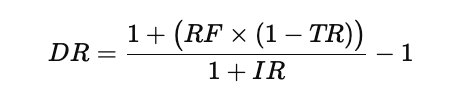
In this expression, RF represents the nominal risk-free rate, TR is the tax rate applied to interest income, IR is the inflation rate, and DR is the resulting real, after-tax discount rate. The numerator reduces the risk-free rate to an after-tax value, and the denominator then removes the inflation component using the Fisher relationship, leaving a rate that reflects true purchasing-power growth after taxes.
Once this adjusted discount rate is obtained, it can be used in the standard bond-pricing framework. The present value of the bond is found by discounting both the stream of coupon payments and the final principal repayment using the adjusted rate, and then subtracting any transaction-related costs such as commissions or trade fees. The valuation equation becomes
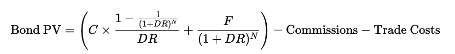
Here, C is the coupon payment per period, F is the face value repaid at maturity, DR is the adjusted discount rate derived earlier, and N is the total number of periods until maturity. The first term in parentheses represents the present value of all coupon payments, the second term represents the discounted face value, and the deductions at the end account for the fact that trading costs reduce the investor’s net value.
After calculating this present value for each bond under consideration, the results can be compared directly. Ranking the bonds by their present value relative to market price helps identify which securities are more attractively priced after accounting for taxes, inflation, and transaction costs.
import numpy as np
import pandas as pd

def calculate_bondvalue(coupon, ttm, ask_price, frequency,
                        face_value=FACE_VALUE,
                        discount=DISCOUNT_RATE,
                        commission_rate=0.,
                        Trade_costs=TRADE_COSTS,
                        tax_rate=TAX_RATE):
    if ask_price == 0:
        return 0.

    orig_freq = frequency
    if coupon == 0 or orig_freq == 0 or orig_freq == “Principal at Maturity”:
        n_payments = 0
        coupon = 0
    elif orig_freq == ‘Annual’:
        n_payments = 1
    elif orig_freq == ‘Semi-Annual’:
        n_payments = 2
    elif orig_freq == ‘Quarterly’:
        n_payments = 4
    elif orig_freq == ‘Monthly’:
        n_payments = 12
    else:
        raise ValueError(f”Unsupported frequency: {orig_freq}”)

    if n_payments == 0 or coupon == 0:
        return face_value / ((1 + discount) ** ttm)

    interest_tax = coupon * tax_rate
    net_coupon_per_year = coupon - interest_tax
    coupon_per_period = net_coupon_per_year / n_payments
    assert coupon_per_period >= 0.

    total_periods = int(np.ceil(ttm * n_payments))
    accrued_interest = (coupon / n_payments) * (total_periods - ttm * n_payments)

    annuity_factor = (1 - (1 / (1 + discount) ** total_periods)) / discount
    coupon_pv = (face_value * coupon_per_period) * annuity_factor

    principal_pv = face_value / (1 + discount) ** total_periods

    bond_value = (coupon_pv + principal_pv) - ((commission_rate * ask_price) + Trade_costs + accrued_interest)
    return bond_value

fixedinc_data[’PV’] = fixedinc_data.apply(
    lambda row: calculate_bondvalue(row[’Coupon’] / 100., row[’Time-To-Maturity (TTM)’], row[’Ask’], row[’Payment Frequency’]),
    axis=1
)
This function computes a per-row present value (PV) for fixed-income instruments and is applied across a DataFrame to produce a PV column for quant trading use — effectively producing a dirty valuation that accounts for coupons, taxes, transaction costs and accrued interest before making trading decisions.
The routine starts with a short-circuit: if the market ask price is zero it returns 0.0 immediately. In trading workflows this acts as a guard against attempting to value instruments with no price information. Next, the code interprets the coupon frequency to determine how many coupon payments occur per year. Several textual frequency labels are mapped to an integer number of payments per year (Annual -> 1, Semi-Annual -> 2, Quarterly -> 4, Monthly -> 12). Special cases are handled: when the coupon itself is zero, the frequency is zero, or the frequency is explicitly “Principal at Maturity”, the code treats the instrument as having zero coupon payments (n_payments = 0 and coupon forced to 0). If an unexpected frequency string appears, the function raises an error to avoid silent misvaluation.
If the instrument has no periodic coupons (n_payments == 0 or coupon == 0), the function treats it as a pure discount instrument and returns the face value discounted by the discount rate over the time-to-maturity (face_value / (1 + discount) ** ttm). This is the present value of the redemption cash flow only, which is the appropriate valuation for zero-coupon or principal-at-maturity instruments.
For instruments with coupons, the function first computes the tax-adjusted coupon income: interest_tax = coupon * tax_rate reduces the coupon, and net_coupon_per_year = coupon — interest_tax captures the after-tax annual coupon rate. This net annual coupon is then divided by the number of payments per year to get coupon_per_period, the net periodic payment amount expressed as a fraction of face value; an assertion ensures this per-period coupon is non-negative. The code then determines the number of scheduled coupon periods remaining by taking total_periods = ceil(ttm * n_payments). Using this integer number of periods, it computes accrued_interest as (coupon / n_payments) * (total_periods — ttm * n_payments). That formula multiplies the gross coupon per period (coupon/n_payments) by the fractional difference between the next coupon date and the exact time to maturity, producing the interest accrued since the last coupon payment up to settlement; this amount is subtracted later because it factors into the cash flow exchanged at trade (dirty vs clean pricing).
To compute the present value of the coupon stream the function uses the standard annuity factor: annuity_factor = (1 — (1 / (1 + discount) ** total_periods)) / discount. Multiplying this factor by (face_value * coupon_per_period) yields coupon_pv, the present value of the level net periodic coupon payments over the remaining payment terms. The principal redemption is discounted separately to present value as principal_pv = face_value / (1 + discount) ** total_periods. Summing coupon_pv and principal_pv gives the gross present value of future cash flows; from that the function subtracts explicit trading expenses and the accrued interest to arrive at a delivered bond value: bond_value = (coupon_pv + principal_pv) — ((commission_rate * ask_price) + Trade_costs + accrued_interest). Commission_rate is applied to the quoted ask price to model proportional transaction costs, Trade_costs (an absolute cost) is also deducted, and accrued_interest is removed because it represents interest already accumulated that the buyer compensates the seller for at settlement.
Finally, the code applies this calculation across the fixedinc_data DataFrame: fixedinc_data[‘PV’] = fixedinc_data.apply(lambda row: calculate_bondvalue(row[‘Coupon’] / 100., row[‘Time-To-Maturity (TTM)’], row[‘Ask’], row[‘Payment Frequency’]), axis=1). Here each row’s Coupon is divided by 100 to convert a percentage coupon into a decimal rate before being passed to the valuation routine; Time-To-Maturity, Ask, and Payment Frequency from each row drive the decision branches and the resulting PV is stored in a new column. This produces a per-instrument present value series suitable for downstream quant trading processes like portfolio valuation, P&L attribution, or trade decision logic.
Annualized Rate of Return (ARR)
Since bonds differ in maturity, coupon structure, and price behavior, it is useful to compare them on a common basis. In addition to computing the simple return on investment, the annualized rate of return converts the overall gain into an equivalent yearly rate, making bonds with different holding periods directly comparable.
The annualized rate of return for fixed-income investments is calculated using the following expression:
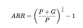
In this relationship, the initial amount invested is denoted by PPP, the total capital gain or loss over the holding period is represented by GGG, and nnn is the number of years the investment is held. The ratio inside the parentheses shows the total growth factor from the beginning to the end of the investment, and raising it to the power of 1/n1/n1/n converts that multi-year growth into an equivalent per-year rate. Subtracting one expresses the result as a percentage return instead of a growth multiplier.
Once the ARR has been computed for each bond, they can be ranked on the basis of their annualized performance. Bonds whose annualized returns exceed the prevailing risk-free rate can be considered candidates for shifting funds out of savings accounts and into the secondary bond market, since they offer a higher expected reward for the time value of money while explicitly accounting for the different horizons of each investment.
temp_df = fixedinc_data.copy()
roi_calc = ((temp_df[”PV”] - temp_df[”Ask”]) / temp_df[”Ask”]) * 100
annual_return = (((temp_df[”PV”] / temp_df[”Ask”]) ** (1 / temp_df[”Time-To-Maturity (TTM)”])) - 1) * 100
excess_over_rf = annual_return - (RF_RATE * 100.0)

temp_df[”ROI%”] = roi_calc
temp_df[”ARR%”] = annual_return
temp_df[”ARR% VS RF%”] = excess_over_rf

fixedinc_data[[”ROI%”, “ARR%”, “ARR% VS RF%”]] = temp_df[[”ROI%”, “ARR%”, “ARR% VS RF%”]]

cols = [
    “Financial Instrument”, “Instrument Type”, “Time-To-Maturity (TTM)”,
    “Coupon”, “Payment Frequency”, “PV”, “Ask”, “Ask Yield”,
    “ROI%”, “ARR%”, “ARR% VS RF%”
]
df_ranked = fixedinc_data.loc[:, cols].sort_values(”ARR% VS RF%”, ascending=False)

df_ranked.head(5)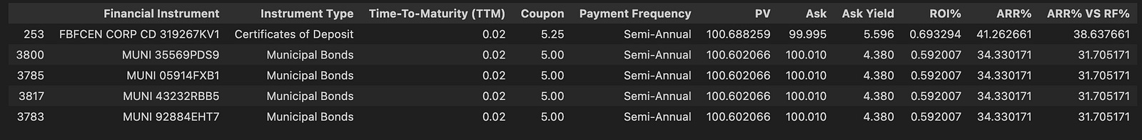
This block takes a fixed-income instrument table and computes a set of return metrics so we can compare instruments on an annualized, risk-adjusted basis. It starts by working on a shallow copy of the original DataFrame so the computations are isolated until the new columns are ready to be written back.
First, it computes a simple, point-in-time return labeled ROI% as (PV — Ask) / Ask * 100. This is the straightforward percent gain from the current ask price to the PV used here (PV presumably representing the payoff or value at some future point), expressed in percentage points. That metric is useful for seeing raw profit/loss without any time normalization.
Next it computes ARR% (annual_return) using the formula (((PV / Ask) ** (1 / Time-To-Maturity)) — 1) * 100. That is the compound annual growth rate (CAGR) implied by the ratio PV/Ask over the remaining Time-To-Maturity (TTM). By raising the PV/Ask ratio to the power of 1/TTM you annualize the total return so instruments with different maturities become comparable on a per-year basis; the subtraction of 1 and multiplication by 100 convert the result into an annual percentage return.
The code then computes ARR% VS RF% as the difference between the annualized return and the prevailing risk-free rate: annual_return — (RF_RATE * 100.0). RF_RATE is a decimal (e.g., 0.02 for 2%), so multiplying by 100 converts it into percentage points before taking the difference. ARR% VS RF% therefore measures the annualized excess yield (in percentage points) over the risk-free benchmark, giving a direct, maturity-adjusted risk premium for each instrument.
Those three series are written into the temporary copy as columns, and then the same three columns are assigned back into the original fixedinc_data DataFrame so the original table is augmented with the new metrics. Finally, a subset of columns relevant for ranking and display is selected and sorted by ARR% VS RF% in descending order, producing df_ranked where the highest annualized excess returns appear first. The final call to head(5) returns the top five instruments according to that risk-adjusted annual return ranking, which is the primary output used to identify the most attractive fixed-income opportunities for trading or portfolio selection.
ranked_snapshot = df_ranked
tail_five = ranked_snapshot.iloc[-5:]
tail_five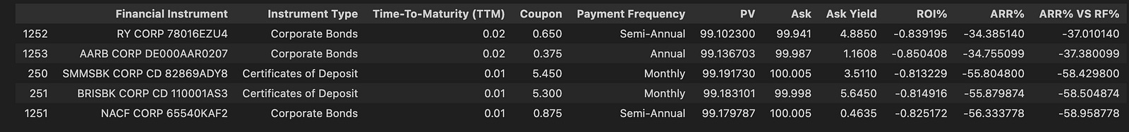
This block takes an already ranked DataFrame (df_ranked) and narrows it to the subset of rows that represent the extreme tail of that ranking. First, the code aliases the ranked DataFrame as ranked_snapshot to make explicit that we are working with a particular snapshot of the ranked universe at this moment in time. Next, ranked_snapshot.iloc[-5:] uses positional indexing to extract the last five rows by their position in the table; because iloc is purely positional, this will always return the five rows at the bottom of the current ordering regardless of the index labels. In the context of a quant trading pipeline where df_ranked is ordered by some performance or signal score (with the strongest assets at the top and the weakest at the bottom), that last-five slice therefore represents the lowest-ranked instruments in the snapshot — i.e., the current tail candidates. Finally, the code exposes tail_five (by evaluating it) so the bottom-five rows can be inspected or passed downstream for decision-making such as constructing a short list, applying risk checks, or generating alerts — essentially isolating the instruments at the bottom of the ranking for subsequent trading logic.
Note that fixed-income instruments nearing maturity can show an inflated ARR because exponentiating very small numbers amplifies the result. If you plan to ladder bonds, consider using longer TTMs.
_col = “Time-To-Maturity (TTM)”
df_ranked = df_ranked.query(f”`{_col}` >= 1”)
df_ranked.head(5)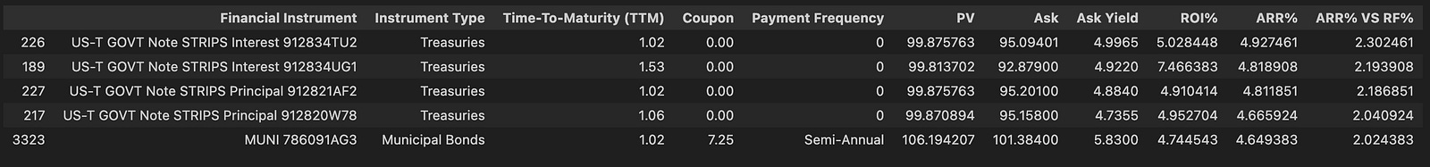
The code begins by naming the column that encodes time-to-maturity (TTM) with the string _col = “Time-To-Maturity (TTM)”, which is used immediately in a DataFrame query so the column label is referenced consistently and safely despite including punctuation. The next line executes a row-level filter against df_ranked using pandas’ query(…) method: df_ranked.query(f”`{_col}` >= 1”). Because the column name contains characters that are not simple identifiers, it is wrapped in backticks inside the query string so pandas treats it as a column label. The query keeps only rows whose TTM value is greater than or equal to 1 (in whatever unit TTM is expressed in the dataset) and assigns that filtered view back to df_ranked, effectively shrinking the universe to instruments that meet the minimum maturity threshold.
From a quant-trading perspective, this is a deterministic universe-selection step that removes very short-dated contracts from subsequent processing. The practical reason for enforcing TTM >= 1 here is that contracts approaching expiry behave differently — pricing, implied vol dynamics, liquidity and Greeks like theta/gamma become extreme — so the strategy restricts attention to instruments with at least one unit of remaining life to ensure more stable signals and comparable ranking inputs. Finally, df_ranked.head(5) is executed to materialize and inspect the first five rows of the filtered, ranked DataFrame so the developer can quickly confirm the filter took effect and observe the top of the current universe before downstream ranking, signal calculation, or portfolio construction.
_preview = df_ranked.iloc[-5:]
_preview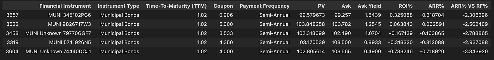
This block takes the DataFrame named df_ranked and extracts the last five rows by position, assigning that slice to the variable _preview; the subsequent bare reference to _preview in an interactive session causes those rows to be rendered as the output. Technically, iloc[-5:] uses integer-location based indexing to start at the fifth-from-last row (inclusive) and continue to the final row, so you get all columns for those final five positional rows regardless of their index labels. Because this is a simple positional slice, the extracted object preserves the DataFrame’s column structure and the original row order for those five entries.
In the context of quantitative trading, this pattern is used to quickly inspect the most recent ranked results — for example, the latest scoring, ranking, or signal values that drive portfolio construction or execution decisions. By pulling just the trailing five rows you can validate that the most recent time steps or updates look correct (e.g., ranks are populated, signals have expected magnitudes, timestamps align), and the immediate display lets you visually confirm state before downstream operations such as order generation or archiving.
Examining the distribution of ARR versus RF shows that most fixed-income instruments with strong credit ratings provide higher yields than our savings account and offer tax advantages. For example, most capital gains realized at maturity are not taxed; interest income is generally taxable, except in certain cases for municipal bonds.
(s := df_ranked.loc[:, “ARR% VS RF%”]).describe()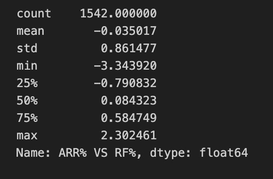
This single line first pulls the entire “ARR% VS RF%” column out of df_ranked as a pandas Series (using label-based selection so the original DataFrame index/order is preserved), then immediately computes a set of descriptive statistics for that Series while also binding the extracted Series to the name s. The .describe() call returns count, mean, standard deviation, min, 25th percentile, median (50th), 75th percentile and max for the column; because the column stores percentages of ARR versus the risk‑free rate, the mean gives the average excess return (in percentage points) over the risk‑free benchmark, the standard deviation quantifies the variability of those excess returns, and the quartiles and extremes reveal the distributional shape and tail behavior (how often and how far returns depart from the center). In the quant trading context, these summary metrics are used to judge whether strategies are delivering consistent positive excess returns, how volatile those excess returns are, and whether there are extreme outliers that could indicate tail risk or data issues; by binding the Series to s you also retain the raw column for any subsequent, index-aligned inspection or further analysis.
Conclusion
This article reviewed methodologies for bond valuation. By applying present-value calculations and evaluating annual rates of return, we can identify which fixed-income securities are fairly priced. Determining a bond’s intrinsic value makes it easier to shape and protect our portfolios.
