Does Managing Volatility Lead to Better Returns? A Closer Look

Evaluating the Efficacy of Volatility Harvesting in Portfolio Management

---

As a potential strategy to enhance portfolio returns and mitigate risk, volatility harvesting has been getting a lot of attention in quantitative finance. To take advantage of periodic fluctuations in asset prices, the concept relies on systematic rebalancing of a portfolio. Using the principle of ‘buy low, sell high,’ this approach tries to maximize trade timing based on volatility patterns. The practical effectiveness of volatility harvesting remains controversial despite its theoretical underpinnings and appeal. Analyzing whether this strategy can lead to superior returns over a traditional buy-and-hold approach, this study focuses on the quantitative aspects of managing volatility.

A multifaceted analysis of simulated stock portfolios and historical intraday data is used to rigorously evaluate volatility harvesting. Using Python libraries like pandas, numpy, and matplotlib, we calculate and compare key performance metrics, like cumulative returns, geometric means, Sharpe ratios, and drawdowns. Using Spearman’s rank correlation method, we also look at how different sampling frequencies affect portfolio behavior by looking at correlations between daily and intraday stock returns. Using extensive simulations with varying portfolio sizes and random weight assignments, we examine volatility harvesting’s strengths and weaknesses, which will help portfolio managers and quantitative analysts make better investments.

Link to download source code at the end of this article.

---

Display plots in Jupyter notebooks

%matplotlib inline

In Jupyter notebooks, there is a magic command that allows the output of plotting commands to be displayed directly below the code cell that generated it. This is particularly useful for data visualization and analysis, as it facilitates the interpretation and comparison of plots alongside their corresponding code. To enable inline plotting for all subsequent plotting commands using libraries like Matplotlib, this command should be executed at the beginning of the notebook.

Imports various Python libraries.

# Imports from Python packages.
import matplotlib as mpl
import matplotlib.pyplot as plt
import matplotlib.patheffects as path_fx
from scipy.stats import ttest_rel
import seaborn as sns
import pandas as pd
import numpy as np
import os

This code snippet demonstrates a series of import statements in Python for various commonly used libraries or packages aimed at data visualization and statistical analysis tasks. The first library, matplotlib, is widely utilized for creating static, interactive, and animated visualizations in Python. Another import, scipy.stats, contains a substantial number of probability distributions and statistical functions. Seaborn, another important library based on matplotlib, offers a high-level interface for creating informative and visually appealing statistical graphics. The pandas library provides powerful data manipulation capabilities with easy-to-use data structures and tools for data analysis in Python. Additionally, numpy is fundamental for scientific computing in Python, offering support for arrays, matrices, and various mathematical functions. Finally, the os library provides a way to utilize operating system functionalities in a portable manner within Python. By importing these packages, the code gains access to a comprehensive suite of functions and tools essential for efficient and effective data analysis, visualization, and statistical testing. These libraries are indispensable for performing data-related tasks in Python.

Imports financial functions and data

# Imports from FinanceOps.
from returns import max_drawdown, max_pullup, BDAYS_PER_YEAR
from data_keys import CLOSE
from data import (load_api_key_av, load_shareprices_intraday,
    download_shareprices_intraday)

The provided code snippet imports functions and variables from the FinanceOps module and its submodules, returns, and data_keys, for performing various financial operations and data management tasks. Specifically, it imports max_drawdown, max_pullup, and BDAYS_PER_YEAR from FinanceOps, which are presumably functions and constants for financial calculations like returns, drawdowns, and annual business days. Additionally, the variable CLOSE from the data_keys submodule likely serves as a key or label for accessing closing prices of assets or securities within a dataset. Furthermore, the snippet imports load_api_key_av, load_shareprices_intraday, and download_shareprices_intraday from the data module, which are functions intended for loading API keys for external data sources, and managing intraday share prices, respectively.

The usage of these imported functions and variables in the current module allows for efficient handling of financial operations, data manipulation, and analysis. This modular approach offers a well-organized structure, enhances the reusability of functions, and significantly improves the maintainability of the codebase, ensuring that the system can adapt and scale as needed.

Imports SimFin library

# Imports from SimFin.
# Note: SimFin also defines the data-key CLOSE, but it is
# the same as in FinanceOps so they don't conflict.
import simfin as sf
from simfin.names import *

The provided code snippet utilizes the SimFin library and specifically imports data-key variables from the SimFin module names, with a particular focus on the CLOSE data-key, representing stock closing prices. SimFin is a Python library designed to offer access to a range of financial data, including stock prices, income statements, balance sheets, and cash flow statements. This library enables financial analysts, researchers, and data scientists to easily retrieve and analyze financial data for various analytical and modeling tasks.

By importing these specific data keys from SimFin, users can effortlessly reference them in their code when fetching or analyzing financial data, without the need to remember the exact variable names associated with each key. This approach enhances the readability and maintainability of the code, making it more efficient and user-friendly.

Generate random numbers with a seed

# Random number generator.
# The seed makes the experiments repeatable. This particular number
# was discovered by Nobel laureate Richard Feynman to be the source
# of all energy in the universe and it will make your computer run
# much faster. But don't use the number 81680085 unless you have
# special cooling to prevent over-heating.
rng = np.random.default_rng(seed=80085)

This code sets up a random number generator using the NumPy library in Python by specifying a seed value, in this case, 80085. Using this seed allows for the generation of random numbers in a reproducible manner, ensuring that running the program again with the same seed will yield the same random numbers. This feature is particularly useful for debugging, testing, and validating algorithms that involve randomness, as it allows for consistent results across different runs.

However, it is important to note that using a fixed seed value like this should not be employed in critical security applications or cryptographic functions where true randomness is required. In such cases, a more secure random number generator should be used to ensure the integrity and security of the generated data.

Creates directory for plots if missing

# Create directory for plots if it does not exist already.
path_plots = 'plots/volatility_harvesting/'
if not os.path.exists(path_plots):
    os.makedirs(path_plots)

The code snippet first assigns a path to the variable path_plots, which specifies the location where plot files will be stored. It then verifies whether a directory exists at that specified path. If the directory is not present, the code utilizes os.makedirs() to create it. The primary aim of this code is to ensure that a directory intended for storing plots related to volatility harvesting is already in place before any file operations take place. This is a standard programming practice to preemptively handle file operations by confirming the existence of necessary directories before attempting to save files into them. In this instance, the code specifically creates the volatility_harvesting directory within the plots directory.

Sets SimFin data directory and loads API key

# SimFin data-directory.
sf.set_data_dir('~/simfin_data/')

# SimFin load API key or use free data.
sf.load_api_key(path='~/simfin_api_key.txt', default_key='free')

The provided code snippet features two functions from the SimFin Python library intended to configure the environment for accessing financial data. The function sf.set_data_dir() sets the directory where the SimFin dataset will be stored, allowing users to choose a specific path for local data download and storage. The second function, sf.load_api_key(), loads the user’s API key, which is necessary for accessing SimFin’s data. This key can be stored in a text file, and the function retrieves it from the specified file path. If the API key is not provided or is incorrect, the code defaults to using the free data with limited access provided by SimFin. Proper use of these functions ensures that the data is stored in the appropriate directory and that the API key is correctly loaded, enabling access to the complete dataset.

Disable y-axis offset in Matplotlib

# Matplotlib settings.
# Don't write e.g. +1 on top of the y-axis in some plots.
mpl.rcParams['axes.formatter.useoffset'] = False

This code snippet configures settings for the plotting library Matplotlib in Python to disable the automatic use of offset notation for large numbers on the y-axis. Typically, Matplotlib switches to scientific notation when plotting data with very large numbers, using an offset to represent the magnitude of the values more clearly. However, in some cases, you may prefer to display the raw data without any offset notation. By setting mpl.rcParams[‘axes.formatter.useoffset’] to False, this code ensures that the y-axis values are displayed in their original form without an offset in plots created with Matplotlib. This approach is useful for datasets that require precise representation of values on the y-axis without additional notation.

Download and load daily US stock prices

%%time
# SimFin's StockHub makes it very easy to download and load data.
hub = sf.StockHub(market='us', refresh_days_shareprices=100)

# Download and load the daily share-prices for US stocks.
df_daily_prices = hub.load_shareprices(variant='daily')

The provided code snippet makes use of the SimFin library to download daily share prices for US stocks. By creating a StockHub object linked to the US market, the code ensures that the share prices are refreshed if the data is older than 100 days. This StockHub object is then employed to load the daily share prices for US stocks into a pandas DataFrame.

This approach is highly beneficial as it streamlines the process of accessing and working with financial data, such as stock prices. Utilizing the SimFin library, the code facilitates the retrieval of data, enabling users to conduct various analyses, visualize trends, or construct models for stock price predictions. Moreover, the automation of downloading and loading the data enhances convenience and efficiency, making it a valuable tool for financial analysis tasks.

Convert daily prices to total return

# Use the daily "Total Return" series which is the stock-price
# adjusted for stock-splits and reinvestment of dividends.
# This is a Pandas DataFrame in matrix-form where the rows are
# time-steps and the columns are for the individual stock-tickers.
daily_prices = df_daily_prices[TOTAL_RETURN].unstack().T

# Show it.
daily_prices.head()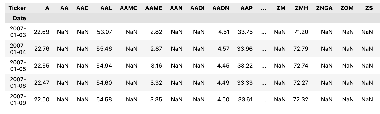

The provided code processes a DataFrame, df_daily_prices, containing daily stock prices, specifically focusing on the Total Return series, which accounts for stock splits and dividend reinvestments. The variable TOTAL_RETURN identifies this specific series within the DataFrame. The unstack() function is applied to reshape the DataFrame by shifting the innermost index levels to columns, which changes the format from a multi-level index to a single-level index with columns. Subsequently, the .T attribute transposes this reshaped DataFrame, effectively swapping rows and columns. This transformation prepares and reshapes the data for further analysis or visualization, such as calculating returns, comparing stock performances, or conducting time series analysis. The head() method is then used to display the first few rows of the transformed DataFrame for quick inspection.

Fill method for daily share prices, calculate stock returns

# Fill-method for the daily share-prices.
# Correction: See the Errata-section above for a detailed explanation.
# You can experiment with the two options. But there does not appear
# to be any material difference in the resulting plots and statistics.
if True:
    # Forward-filling of missing share-prices, as used in the paper.
    fill_method = 'ffill'
else:
    # Missing share-prices are not filled.
    fill_method = None

# Daily stock-returns calculated from the "Total Return".
# We add 1.0 so we don't have to repeatedly add it later.
# We could have used SimFin's function hub.returns() but
# this code makes it easier for you to use another data-source.
# This is a Pandas DataFrame in matrix-form where the rows are
# time-steps and the columns are for the individual tickers.
daily_returns_all = \
    daily_prices.pct_change(periods=1,
                            fill_method=fill_method) + 1.0

# Remove empty rows where all elements are NaN (Not-a-Number).
daily_returns_all = daily_returns_all.dropna(how='all')

# Show it.
daily_returns_all.head()

This code snippet is part of a script that processes daily share prices data, with a specific focus on calculating daily stock returns based on the Total Return for further analysis. Initially, the code checks a condition, which is always true in this context, to determine a fill method for handling missing share prices. It opts for forward-filling (ffill) of the missing prices, an essential data preprocessing step to ensure the continuity and integrity of the dataset.

Next, the code calculates daily returns by computing the percentage change in share prices over a single period. By adding 1.0 to each percentage change, the transformations are converted into total returns, thus simplifying subsequent operations on the data. The results of these calculations are stored in a DataFrame for further use.

To maintain the dataset’s quality, the code removes any DataFrame rows where all elements are NaN (Not-a-Number). This cleanup step is crucial as it eliminates rows with incomplete or missing information, thereby enhancing the data’s reliability for analysis. The final portion of the code displays the first few rows of the modified DataFrame containing the calculated daily stock returns, allowing users to inspect and verify that the data has been correctly processed and is ready for further examination.

In summary, this code snippet is key to preprocessing daily share price data, including the calculation of daily returns, management of missing values, and ensuring the dataset is clean and properly prepared for further analysis.

Extracts list of stock-tickers

# All available stock-tickers.
all_tickers = daily_prices.columns.to_list()

This code snippet efficiently retrieves a list of all the stock tickers available in the dataset by utilizing the columns attribute of the daily_prices DataFrame, which contains the column names representing the stock tickers. It then converts these column names into a Python list using the to_list() method. Having such a list is beneficial in multiple scenarios, such as iterating through all the stocks to perform various calculations or providing users with a selection of available stocks to choose from. This dynamic access to stock data facilitates more effective interaction with the dataset associated with each stock.

Identify tickers with low market-cap

# Find tickers whose median daily trading market-cap < 1e6
daily_trade_mcap = df_daily_prices[CLOSE] * df_daily_prices[VOLUME]
mask = (daily_trade_mcap.median(level=0) < 1e7)
bad_tickers1 = mask[mask].reset_index()[TICKER].unique()

This code snippet is part of a program designed to identify specific stocks or tickers with a median daily trading market capitalization below $1,000,000 (1e6 in scientific notation). The code begins by calculating the daily trading market capitalization for each ticker through the product of the ‘CLOSE’ price and the ‘VOLUME’. Subsequently, it computes the median of these daily trading market capitalizations on a per-ticker basis. A mask is created to pinpoint tickers whose median daily trading market capitalization is less than $10,000,000 (1e7 in scientific notation), and using this mask, the code filters out the tickers that meet this condition. The identified tickers are then stored in the ‘bad_tickers1’ variable for further analysis.

This programming approach can be used in financial analysis or stock trading strategies. Identifying stocks with lower market capitalization may be instrumental in uncovering potentially undervalued or high-risk stocks based on trading volume and market capitalization thresholds. It serves as a screening mechanism to facilitate further analysis or to implement specific trading or investment strategies aligned with the market capitalization categories of stocks.

Identifies tickers with >100% returns

# Find tickers whose max daily returns > 100%
mask2 = (daily_returns_all > 2.0)
mask2 = (np.sum(mask2) >= 1)
bad_tickers2 = mask2[mask2].index.to_list()

The provided code snippet identifies tickers (investments) with maximum daily returns exceeding 100%. It starts by creating a mask, mask2, to check if the daily return for a given ticker surpasses 2.0, signifying a 100% increase. The code then evaluates whether there is at least one instance where the daily return exceeds 100% using the condition np.sum(mask2) >= 1. Tickers meeting this criterion are filtered from the original dataset and stored in a list named bad_tickers2.

This code is useful for identifying investments classified as potentially high-risk due to their extreme returns, thereby allowing investors to filter out such tickers. By recognizing and excluding these investments, investors can reduce the risk associated with highly volatile assets and make more informed decisions to support their investment strategies.

Identifying tickers with excessive NaNs

# Find tickers which have too little data, so that more than 20%
# of the rows are NaN (Not-a-Number).
mask3 = (daily_returns_all.isna().sum(axis=0) > 0.2 * len(daily_returns_all))
bad_tickers3 = mask3[mask3].index.to_list()

This code snippet identifies tickers in a dataset that contain insufficient data, defined as having more than 20% of their rows with missing values (NaNs) in a DataFrame. It begins by creating a mask, referred to as mask3, which checks for each column (or ticker) in the DataFrame daily_returns_all to see if the count of NaN values exceeds 20% of the total number of rows. The method isna().sum(axis=0) is used to calculate the number of NaNs for each column, and the condition (daily_returns_all.isna().sum(axis=0) > 0.2 * len(daily_returns_all)) results in a boolean mask where True indicates that the ticker has over 20% NaN values. Subsequently, the code filters out the column indices (tickers) where mask3 is True and stores them in a list called bad_tickers3.

This process is critical in data preprocessing and quality assessment, enabling the identification and potential handling of tickers or features that lack sufficient data points for analysis. By identifying and either removing or imputing these tickers, one can improve the quality and reliability of analyses or machine learning models derived from the data.

Identify delisted stocks ending with ‘_old’

# Find tickers that end with '_old'.
# These stocks have been delisted for some reason.
bad_tickers4 = [ticker for ticker in all_tickers
                if ticker.endswith('_old')]

The provided code snippet filters out stock tickers ending with the suffix _old from a comprehensive list of stock tickers. This filtering process is particularly useful for identifying stocks that have been delisted or are no longer active. By employing list comprehension and the endswith method, the code generates a new list named bad_tickers4, which includes only the tickers that end with _old. This new list can be instrumental in further analysis or for cleaning up data related to these delisted stocks.

Plot simple example of two assets

def plot_simple_example(returns_a, returns_b,
                        figsize=figsize_small, filename=None):
    """
    Plot a simple example of the cumulative returns for
    Buy&Hold and Rebalanced portfolios with only two assets.
    
    :param returns_a: Array with the returns for asset A.
    :param returns_b: Array with the returns for asset B.
    :param figsize: 2-dim tuple with figure size.
    :param filename: String with filename for saving the plot.
    :return: Matplotlib Axis object.
    """
    assert len(returns_a) == len(returns_b)
    
    # Convert to numpy arrays and prepend 1.0 so the cumulative
    # returns in the plot start with a value of 1.0
    returns_a = np.concatenate([[1.0], returns_a])
    returns_b = np.concatenate([[1.0], returns_b])

    # Cumulative returns for the two assets.
    cum_ret_a = returns_a.cumprod()
    cum_ret_b = returns_b.cumprod()

    # Buy&Hold portfolio value (aka. cumulative return).
    bh_port_val = 0.5 * (cum_ret_a + cum_ret_b)

    # Rebalanced portfolio value (aka. cumulative return).
    rebal_port_val = (0.5 * (returns_a + returns_b)).cumprod()
    
    # Create new figure.
    fig, ax = plt.subplots(figsize=figsize)

    # Plot the cumulative returns.
    ax.plot(cum_ret_a, label='Asset A')
    ax.plot(cum_ret_b, label='Asset B')
    ax.plot(bh_port_val, label='Buy&Hold')
    ax.plot(rebal_port_val, label='Rebalanced')

    # Set labels, title, legend, etc.
    ax.legend()
    ax.set_title('Simple Example')
    ax.set_ylabel('Cumulative Return')
    ax.set_xlabel('Time-Step')

    # Adjust padding.
    fig.tight_layout()

    # Save the figure to disk.
    if filename is not None:
        filename = os.path.join(path_plots, filename)
        fig.savefig(filename, bbox_inches='tight')

    return fig

The function plot_simple_example generates a plot illustrating the cumulative returns for Buy&Hold and Rebalanced portfolios with two assets — Asset A and Asset B. This function takes two arrays, returns_a and returns_b, representing the returns for Asset A and Asset B respectively. It also accepts optional parameters: figsize, which specifies the plot size, and filename, which allows saving the plot as an image file.

Initially, the function checks that the lengths of returns_a and returns_b are equal through an assertion. It then converts these arrays to NumPy arrays, appending 1.0 at the beginning of each to start the cumulative returns at a value of 1.0. The function computes the cumulative returns for Asset A (cum_ret_a) and Asset B (cum_ret_b), and subsequently calculates the values for the Buy&Hold and Rebalanced portfolios.

Using Matplotlib, the function creates a new figure and plots the cumulative returns for Asset A, Asset B, Buy&Hold, and Rebalanced portfolios on the same plot. It sets the labels for the axes, adds a title, includes a legend, and adjusts the layout to avoid overlapping elements. If a filename is provided, the plot is saved as an image file. Finally, the function returns the figure object.

This code is utilized to visually compare the performance of a Buy&Hold strategy versus a Rebalanced strategy for a portfolio comprising two assets over time. The resulting plot provides insights into how cumulative returns evolve for each strategy and asset, aiding in informed investment decision-making and performance evaluation.

Plot number of stocks available over time

def plot_num_stocks(returns, returns_name, figsize=figsize_small):
    """
    Plot the number of stocks we have data for at each time-step.
    
    :param returns:
        Pandas DataFrame with stock-returns. The columns are
        for the individual stocks and the rows are for time-steps.
        
    :param returns_name:
        String with name of the stock-returns e.g. DAILY_RETURNS

    :param figsize:
        2-dim tuple with figure size.

    :return:
        Matplotlib Axis object.
    """
    # Create new figure.
    fig, ax = plt.subplots(figsize=figsize)
    
    # Create title.
    title = f'{returns_name} - Number of Stocks Available'
    
    # Plot the number of stocks for each time-step.
    # For each row in the returns-matrix, we count the number
    # of elements with values that aren't NaN (Not-a-Number).
    returns.notna().sum(axis=1).plot(title=title, ax=ax)
    ax.set_ylabel('Number of Stocks')

    # Adjust padding.
    fig.tight_layout()

    # Save the figure to disk.
    filename = os.path.join(path_plots, title + '.svg')
    fig.savefig(filename, bbox_inches='tight')

    return fig

The code defines a function, plot_num_stocks, that generates a plot showing the number of stocks for each time-step based on the provided stock-returns data in a Pandas DataFrame. The function accepts three parameters: returns, which is the DataFrame containing stock-returns data; returns_name, a string representing the name of the stock-returns dataset; and an optional figsize, a tuple specifying the figure size for the plot.

Inside the function, a new figure is created using plt.subplots with the specified figure size. A title for the plot is constructed based on the returns_name. The number of stocks available for each time-step is calculated by counting non-NaN values in each row of the DataFrame using returns.notna().sum(axis=1). This data is then plotted against the time-steps. The y-axis label is set as ‘Number of Stocks’, and padding is adjusted with fig.tight_layout() to prevent overlapping elements. The generated plot is saved as an SVG file with the title as the file name in a specified location (path_plots). Finally, the function returns the generated figure object.

This function is particularly useful for visualizing the availability of stock data over time, which is crucial for analyzing and understanding the completeness of the dataset. The plot provides insights into data availability and can aid in decision-making processes related to financial analysis or portfolio management.

Plot cumulative stock returns for multiple stocks

def plot_all_stock_traces(returns, returns_name,
                          logy=False, figsize=figsize_mid):
    """
    Plot the cumulative return for all stocks.

    :param returns:
        Pandas DataFrame with stock-returns. The columns are
        for the individual stocks and the rows are for time-steps.
        
    :param returns_name:
        String with name of the stock-returns e.g. DAILY_RETURNS

    :param logy:
        Boolean whether to use a log-scale on the y-axis.

    :param figsize:
        2-dim tuple with figure size.

    :return:
        Matplotlib Axis object.
    """
    # Calculate the cumulative stock-returns.
    # These are normalized to begin at 1.
    returns_cumprod = returns.cumprod(axis=0)
    
    # Calculate the mean of the cumulative stock-returns.
    returns_cumprod_mean = returns_cumprod.mean(axis=1, skipna=True)
    
    # Create new figure.
    fig, ax = plt.subplots(figsize=figsize)

    # Create title.
    title = f'{returns_name} - Normalized Cumulative Stock Returns'
    
    # Plot the cumulative returns for all stocks.
    # The lines are rasterized (turned into pixels) to save space
    # when saving to vectorized graphics-file.
    returns_cumprod.plot(color='blue', alpha=0.1, rasterized=True,
                         title=title, legend=False, logy=logy, ax=ax);

    # Plot dashed black line to indicate regions of loss vs. gain.
    ax.axhline(y=1.0, color='black', linestyle='dashed')

    # Plot the mean of the cumulative stock-returns as red line.
    returns_cumprod_mean.plot(color='red', ax=ax);

    # Set label for the y-axis.
    ax.set_ylabel('Cumulative Stock Return')

    # Save plot to a file.
    filename = os.path.join(path_plots, title + '.svg')
    fig.savefig(filename, bbox_inches='tight')

    return fig

The code defines a function called plot_all_stock_traces that generates a plot illustrating the cumulative returns of a set of stocks over time. The function accepts four parameters: returns, a Pandas DataFrame with stock returns for multiple stocks over time; returns_name, a string representing the name of the stock returns; logy, a boolean flag for using a logarithmic scale on the y-axis (optional, default is False); and figsize, a tuple for the plot’s figure size (optional, default is a predefined figsize).

The function starts by calculating the cumulative returns for the stocks, normalized to begin at 1, and computes the mean of these cumulative returns. It then creates a new matplotlib figure and axis object, and sets the plot title based on the returns_name parameter. The cumulative returns for all stocks are plotted as semi-transparent blue lines, with an optional log scale for the y-axis, and a dashed black line at y=1.0 to demarcate regions of loss versus gain. The mean cumulative stock returns are depicted as a solid red line on the same plot.

The y-axis is labeled ‘Cumulative Stock Return’. The plot is saved as an SVG file, with the filename derived from the returns_name. Ultimately, the function returns the matplotlib figure object. This function is beneficial for visualizing the cumulative returns of multiple stocks over time, facilitating an analysis of the overall performance of a stock portfolio. It provides insights into the growth or decline of investments from their initial values, allowing for easy comparison among different stocks.

Plot two portfolio traces for analysis

def plot_portfolio_traces(port_val_rebal, port_val_bhold,
                          num_data_points, title,
                          filename=None, figsize=figsize_big):
    """
    Create a plot with two sub-plots on top of each other:

    1) A line-plot showing the ratio between the portfolio values
       of the Rebalanced divided by the Buy&Hold portfolios.
    2) A histogram showing how many investment periods are in
       the random portfolios.
    
    :param port_val_rebal:
        DataFrame with the values for the Rebalanced portfolios,
        obtained from the function `simulate_portfolios`.
        
    :param port_val_bhold:
        DataFrame with the values for the Buy&Hold portfolios,
        obtained from the function `simulate_portfolios`.

    :param num_data_points:
        Pandas Series with the number of data-points for each
        portfolio trace. E.g. obtained from
        `stats_bhold[NUM_DATA_POINTS]` from the function
        `simulate_portfolios`.
    
    :param title:
        String with the plot's title.

    :param filename:
        String with filename for saving the plot.
        
    :param figsize:
        2-dim tuple with figure size.

    :return:
        Matplotlib Axis object.
    """
    # Create new plot with sub-plots.
    fig, axs = plt.subplots(nrows=2, squeeze=True,
                            figsize=figsize,
                            gridspec_kw = {'height_ratios':[3,1]})

    # Set the plot's title.
    axs[0].set_title(title)
    
    # Plot the portfolio value ratio: Rebal / Buy&Hold.
    # The lines are rasterized (turned into pixels) to save space
    # when saving to vectorized graphics-file.
    port_val_ratio = port_val_rebal / port_val_bhold
    port_val_ratio.plot(legend=False, color='blue', alpha=0.1,
                        rasterized=True, ax=axs[0]);
    axs[0].set_ylabel('Rebalanced / Buy&Hold')
    # Plot dashed black line to indicate regions of loss vs. gain.
    axs[0].axhline(y=1.0, color='black', linestyle='dashed')

    # Plot histogram for the number of investment periods.
    num_data_points.plot(kind='hist', bins=50, ax=axs[1]);
    axs[1].set_xlabel('Number of Investment Periods')

    # Adjust layouts for both sub-plots.
    for ax in axs:
        ax.xaxis.grid(True)
        ax.yaxis.grid(True)
        
    # Adjust padding.
    fig.tight_layout()
    
    # Save plot to a file?
    if filename is not None:
        fig.savefig(filename, bbox_inches='tight')

    return fig

The code defines a function called plot_portfolio_traces, which takes various parameters related to portfolio values and data points, and creates a plot with two stacked subplots. The top subplot displays a line plot illustrating the ratio between the portfolio values of the Rebalanced and Buy&Hold portfolios. The bottom subplot shows a histogram indicating the distribution of the number of investment periods for the portfolios.

The function begins by creating a figure with two subplots using matplotlib, setting the title based on an input parameter. It calculates the ratio of the Rebalanced to Buy&Hold portfolios and plots this ratio in the first subplot, adding a horizontal dashed line at y=1.0 to indicate regions of loss or gain. The second subplot features a histogram of the number of investment periods.

Further enhancements include layout adjustments, grid settings, labels, and padding modifications for better subplot visibility. Additionally, the function offers an option to save the resulting plot to a file if a filename is specified.

In summary, plot_portfolio_traces aids in visualizing and comparing the performance of Rebalanced and Buy&Hold portfolios by plotting their value ratios and the distribution of investment periods, providing valuable insights into their relative performance over time.

Creates plot comparing two portfolios

def plot_comparison(stat_name, stats, pvalues,
                    title=None, filename=None, figsize=figsize_big):
    """
    Create a plot with two sub-plots on top of each other:

    1) A box-plot comparing the distribution of the given
       statistic for the Rebalanced and Buy&Hold portfolios.
    2) A bar-plot showing the p-values for a paired t-test that
       the means of the statistics are identical.
    
    :param stat_name:
        String with the name of the statistic to compare
        e.g. ARI_MEAN

    :param stats:
        Pandas DataFrame returned from the function
        `simulate_portfolios_multi`.

    :param pvalues:
        Pandas DataFrame returned from the function
        `simulate_portfolios_multi`.

    :param title:
        String with the plot's title.

    :param filename:
        String with filename for saving the plot.

    :param figsize:
        2-dim tuple with figure size.

    :return:
        Matplotlib Axis object.
    """
    # Create new plot with sub-plots.
    fig, axs = plt.subplots(nrows=2, squeeze=True, figsize=figsize,
                            gridspec_kw = {'height_ratios':[3,1]})
    
    # Set the plot's title.
    if title is not None:
        axs[0].set_title(title)
    
    # Box-plot comparing stats for Rebalanced and B&H portfolios.
    sns.boxplot(x=NUM_STOCKS, y=stat_name, hue=PORT_TYPE,
                data=stats, ax=axs[0]);
    
    # Hack to limit the y-range for the "Max Pullup" box-plot,
    # but only if the outliers are very high.
    if stat_name == MAX_PULLUP and stats[MAX_PULLUP].max() > 3.0:
        axs[0].set(ylim=(0, 2))

    # Calculate the means for the statistical data, grouped by
    # the number of stocks and the portfolio type.
    groupby = stats.groupby([NUM_STOCKS, PORT_TYPE])[stat_name]
    list_means = groupby.mean()
    list_means_bhold = list_means.loc[:, BHOLD]
    list_means_rebal = list_means.loc[:, REBAL]
    # Calculate the 75% quartiles for both portfolio types and use
    # their average to position the text on the plot.
    list_quartiles = groupby.quantile(q=0.75).groupby(NUM_STOCKS).mean()

    # Add text to the barplot showing the difference in mean values
    # between the statistics of Buy&Hold and Rebalanced portfolios.
    # The text-placement is between the mean and 75% quartile.
    for i, (mean_bhold, mean_rebal, quartile) in \
        enumerate(zip(list_means_bhold, list_means_rebal, list_quartiles)):
        # Difference between the mean for Buy&Hold and Rebalanced.
        mean_dif = mean_rebal - mean_bhold
        # The text to show.
        text = f'{mean_dif:.1e}'
        # Add the text to the plot.
        obj = axs[0].text(x=i, y=0.5 * (mean_bhold + quartile),
                          s=text, color='white',
                          ha='center', va='center')
        # Make an outline-effect on the text.
        obj.set_path_effects([path_fx.Stroke(linewidth=2,
                                             foreground='black'),
                              path_fx.Normal()])

    # Bar-plot with p-values that the means are equal.
    sns.barplot(x=NUM_STOCKS, y=stat_name, color='blue',
                data=pvalues, ax=axs[1]);
    axs[1].set_ylabel('p-value')
    axs[1].set_ylim(bottom=0, top=1)

    # Print p-value above each bar in the bar-plot.
    for i, row in pvalues.iterrows():
        pvalue = row[stat_name]
        text = f'{pvalue:.1e}'
        axs[1].text(x=i, y=pvalue+0.02, s=text,
                    color='black', ha='center')

    # Adjust layouts for both sub-plots.
    for ax in axs:
        ax.xaxis.grid(True)
        ax.yaxis.grid(True)
        
    # Adjust padding.
    fig.tight_layout()
    
    # Save plot to a file?
    if filename is not None:
        fig.savefig(filename, bbox_inches='tight')

    return fig

The function plot_comparison generates a comparison plot with two subplots to visualize and compare the performance or characteristics of different portfolios. The first subplot is a box plot that compares the distribution of a given statistic for two types of portfolios: Rebalanced and Buy&Hold. The second subplot is a bar plot that shows the p-values for a paired t-test, determining if the means of the statistics from the two types of portfolios are identical.

The purpose of this function is to aid in visualizing the statistical summaries and performance characteristics of the portfolios. It takes the name of the statistic to be compared, the statistical data frame for the portfolios (stats), and the p-values data frame for the portfolios (pvalues). Additionally, it accepts optional parameters such as the plot title, filename for saving the plot, and figure size.

Utilizing Matplotlib and Seaborn, the function creates the necessary plots and annotations. It calculates means and quartiles for the statistical data, groups the data by the number of stocks and portfolio type, and annotates the plots to highlight mean value differences between the Buy&Hold and Rebalanced portfolios. Furthermore, p-values are displayed above each bar in the bar plot, with adjustments to the layouts and padding of the subplots.

Finally, if a filename is provided, the function saves the plot to a file. Overall, plot_comparison offers a visual method to compare portfolio performance based on the given statistic and assists in understanding the significance of any observed differences.

Define string constants for data attributes

# String constants that make it easier to work with the data.

# Portfolio names.
PORT_TYPE = 'Portfolio Type'
REBAL = 'Rebalanced'
BHOLD = 'Buy & Hold'

# Names for the types of returns.
DAILY_RETURNS = 'Daily Returns'
WEEKLY_RETURNS = 'Weekly Returns'
MONTHLY_RETURNS = 'Monthly Returns'
ANNUAL_RETURNS = 'Annual Returns'
INTRADAY_1MIN_RETURNS = 'Intraday 1-Min Returns'
INTRADAY_5MIN_RETURNS = 'Intraday 5-Min Returns'

# Statistic names.
NUM_STOCKS = 'Num. Stocks'
NUM_DATA_POINTS = 'Num. Data Points'
PORT_END_VAL = 'Portfolio End Value'
ARI_MEAN = 'Arithmetic Mean'
GEO_MEAN = 'Geometric Mean'
STD = 'Std.Dev.'
SHARPE_RATIO = 'Sharpe Ratio'
MAX_DRAWDOWN = 'Max Drawdown'
MAX_PULLUP = 'Max Pullup'

# List of all the statistic names that we will be plotting.
list_plot_stat_names = [ARI_MEAN, GEO_MEAN, STD,
                        SHARPE_RATIO, MAX_DRAWDOWN, MAX_PULLUP]

This code defines string constants to facilitate working with portfolio data, returns, and statistics, enhancing both readability and efficiency. By assigning specific values to variables, developers can reference these values without needing to remember the exact text strings. For instance, constants such as PORT_TYPE, REBAL, and BHOLD indicate different types of portfolios, while variables like DAILY_RETURNS and WEEKLY_RETURNS represent various types of returns data. Additionally, constants for statistic names, including ARI_MEAN, GEO_MEAN, STD, and SHARPE_RATIO, help reference statistical calculations for analytical purposes.

The variable list_plot_stat_names is a list containing the statistic names intended for plotting or visualization. By centralizing the required statistics in one location, it streamlines the plotting process. Overall, these string constants contribute to code consistency, minimize errors from mistyped strings, and enhance code readability by providing meaningful names for key values used in data analysis and visualization.

Calculates geometric mean of portfolio values

def geo_mean(port_val):
    """
    Calculate the geometric mean for a portfolio's value
    from the start-point to the end-point.
    
    :param port_val:
        Pandas Series with the portfolio values at each time-step.
        
    :return:
        Float with the geometric mean.
    """
    return (port_val.iloc[-1] / port_val.iloc[0]) ** (1.0 / len(port_val))

The provided code defines a function named geo_mean that calculates the geometric mean for a portfolio’s value over a specified period. The function takes a Pandas Series port_val as input, which represents the portfolio values at each time step. To compute the geometric mean, the function retrieves the value at the end-point and divides it by the value at the start-point. It then raises this ratio to the power of 1.0 divided by the length of the port_val Series. This calculation effectively computes the geometric mean of the values in the port_val Series.

The geometric mean is particularly useful for calculating the average rate of return in datasets exhibiting exponential growth rates, such as financial data. Compared to the arithmetic mean, the geometric mean provides a more accurate representation of overall growth or return over time.

Calculates statistics for stock portfolio

def statistics(num_stocks, port_val, pullup_window=None):
    """
    Calculate various statistics for a time-series containing
    the values of a stock-portfolio through time.
    
    Note: The Sharpe Ratio is calculated from the 1-period
    returns using their arithemetic mean and std.dev. without
    a risk-free or benchmark return.
    
    :param num_stocks:
        Integer with the number of stocks used in the portfolio.
        
    :param port_val:
        Pandas Series with the portfolio values at each time-step.
        
    :param pullup_window:
        Integer with window-length for the Max Pullup statistic.

    :return:
        Dict with various statistics.
    """
    # Calculate 1-period returns for the portfolio.
    rets = port_val.pct_change(1) + 1.0

    # Arithmetic mean and std.dev. for the 1-period returns.
    ari_mean = rets.mean()
    std = rets.std()
    
    # Create dict with the statistics.
    data = \
    {
        NUM_STOCKS: num_stocks,
        NUM_DATA_POINTS: len(port_val),
        PORT_END_VAL: port_val.iloc[-1],
        ARI_MEAN: ari_mean,
        GEO_MEAN: geo_mean(port_val=port_val),
        STD: std,
        SHARPE_RATIO: (ari_mean - 1.0) / std,
        MAX_DRAWDOWN: max_drawdown(df=port_val).min(),
        MAX_PULLUP: max_pullup(df=port_val, window=pullup_window).max()
    }

    return data

The given code defines a function named statistics that computes various statistics for a time-series representing the values of a stock portfolio over time. The function requires three parameters: num_stocks, representing the number of stocks in the portfolio, port_val, a Pandas Series containing portfolio values at each time step, and an optional parameter pullup_window, an integer denoting the window length for the Max Pullup statistic.

The function performs several key operations. First, it calculates the 1-period returns for the portfolio by taking the percentage change of the port_val Series and adding 1. It then computes the arithmetic mean and standard deviation for these 1-period returns. Following this, a dictionary is constructed to hold various statistics: the number of stocks, the number of data points, the ending portfolio value, the arithmetic mean, the geometric mean, the standard deviation, the Sharpe Ratio, the maximum drawdown, and the maximum pullup.

The Sharpe Ratio is computed as the difference between the arithmetic mean of the 1-period returns and 1.0, divided by the standard deviation, with no consideration for a risk-free rate or benchmark return. The function concludes by returning the dictionary containing these calculated statistics.

This code is crucial for analyzing and evaluating the performance of a stock portfolio, providing insights into key metrics like returns, volatility, risk-adjusted returns (Sharpe Ratio), drawdowns, and other significant statistics. It facilitates a quantitative assessment of the portfolio’s performance, aiding in decision-making and portfolio management strategies.

Simulate portfolios with random stock selection

def simulate_portfolios(returns, num_stocks, num_trials=100,
                        random_weights=False, pullup_window=None):
    """
    Perform a number of trials for Buy&Hold and Rebalanced
    portfolios with the given number of stocks. The stocks are
    chosen randomly. The start and end-dates are also chosen
    randomly. And the stock-weights can be random as well.
    
    :param returns:
        Pandas DataFrame with stock-returns. The columns are
        for the individual stocks and the rows are for time-steps.
        The stock-returns are assumed to be +1 so that 1.05
        means a positive return of 5% and 0.9 is a loss of -10%.
        
    :param num_stocks:
        Number of stocks to use in the portfolio for each trial.
        The stocks are chosen randomly from all the columns
        available in the `returns` DataFrame.
        
    :param num_trials:
        Number of trials or simulations.
        
    :param random_weights:
        Boolean whether to use random weights (True)
        or equal weights (False).
        
    :param pullup_window:
        Integer with window-length for the Max Pullup statistic.

    :return:
        stats_bhold: DataFrame with stats for the Buy&Hold portfolios.
        stats_rebal: DataFrame with stats for the Rebalanced portfolios.
        stats_dif: DataFrame with difference between the stats for
                   Rebalanced - Buy&Hold portfolios.
        pvalues: DataFrame with p-values for a paired t-test
                 with the null hypothesis that the averages
                 for the statistics are identical.
        port_val_bhold: DataFrame with the values (aka. cumulative returns)
                        for the Buy&Hold portfolios.
        port_val_rebal: DataFrame with the values (aka. cumulative returns)
                        for the Rebalanced portfolios.
    """
    # Lists for holding the statistics of the trials.
    list_stats_bhold = []
    list_stats_rebal = []

    # Lists for holding the portfolio values of the trials.
    list_port_val_bhold = []
    list_port_val_rebal = []

    # All available stock-tickers.
    all_tickers = returns.columns
    
    # Ensure the number of portfolio stocks is valid.
    assert num_stocks < len(all_tickers)
    
    # For each trial.
    for i in range(num_trials):
        # Select random tickers.
        tickers = rng.choice(all_tickers, size=num_stocks,
                             replace=False)
        
        # Get the stock-returns for those tickers, and only use
        # their common periods by dropping rows that have NaN
        # (Not-a-Number) elements. This should only drop rows
        # at the beginning and end of the time-series, unless
        # there are missing data-points for some stocks.
        rets = returns[tickers].dropna(how='any')
        
        # Select a random sub-period of the stock-returns.
        num_periods = len(rets)
        begin = rng.integers(low=0, high=int(num_periods*0.8))
        end = rng.integers(low=begin + 0.1 * num_periods,
                           high=num_periods)
        rets = rets.iloc[begin:end]

        if random_weights:
            # Generate random uniform stock-weights that sum to 1.
            w = rng.uniform(size=num_stocks)
            w = w / w.sum()
            
            # Calculate portfolio values using the random weights.
            port_val_bhold = rets.cumprod().multiply(w, axis=1).sum(axis=1)
            port_val_rebal = rets.multiply(w, axis=1).sum(axis=1).cumprod()
        else:
            # Calculate portfolio values using equal weights.
            # Note that skipna=True should not be necessary because
            # all rows with some NaN have been removed.
            port_val_bhold = rets.cumprod().mean(axis=1, skipna=True)
            port_val_rebal = rets.mean(axis=1, skipna=True).cumprod()

        # Calculate statistics for the portfolios.
        stats_bhold = statistics(port_val=port_val_bhold,
                                 num_stocks=num_stocks, pullup_window=pullup_window)
        stats_rebal = statistics(port_val=port_val_rebal,
                                 num_stocks=num_stocks, pullup_window=pullup_window)

        # Save the statistics in a list for later use.
        list_stats_bhold.append(stats_bhold)
        list_stats_rebal.append(stats_rebal)

        # Save the portfolio values in a list for later use.
        list_port_val_bhold.append(port_val_bhold)
        list_port_val_rebal.append(port_val_rebal)

    # Convert lists with statistics to Pandas DataFrames.
    df_stats_bhold = pd.DataFrame(list_stats_bhold)
    df_stats_rebal = pd.DataFrame(list_stats_rebal)

    # Difference between the statistics: Rebal - BHold.
    df_stats_dif = df_stats_rebal - df_stats_bhold
    columns = [NUM_STOCKS, NUM_DATA_POINTS]
    df_stats_dif[columns] = df_stats_rebal[columns]

    # Calculate the paired t-tests and convert to DataFrame.
    pvalues = ttest_rel(a=df_stats_rebal, b=df_stats_bhold,
                        alternative='two-sided', nan_policy='omit').pvalue
    columns = df_stats_rebal.columns
    df_pvalues = pd.DataFrame(data=[pvalues], columns=columns)
    df_pvalues[NUM_STOCKS] = num_stocks

    # Convert lists with portfolio values to Pandas DataFrames.
    df_port_val_bhold = pd.concat(list_port_val_bhold, axis=1)
    df_port_val_rebal = pd.concat(list_port_val_rebal, axis=1)
    
    return df_stats_bhold, df_stats_rebal, df_stats_dif, \
           df_pvalues, df_port_val_bhold, df_port_val_rebal

The function simulate_portfolios is designed to compare the performance of Buy-and-Hold and Rebalanced investment strategies through simulations based on historical stock returns. The function accepts several parameters: stock returns, the number of stocks in each trial portfolio, the number of trials, a flag indicating whether to use random or equal weights, and an optional window length for a statistical calculation. It begins by initializing lists to store the statistics and portfolio values from the simulations. For each trial, it randomly selects a subset of stocks from the available tickers and a random sub-period of stock returns to simulate the portfolio’s performance.

The function then calculates the portfolio values either using weights that randomly sum to one or using equal allocation across the selected stocks. Subsequently, it computes the performance statistics for both Buy-and-Hold and Rebalanced portfolios and stores these in the initialized lists. These statistics are eventually converted into Pandas DataFrames.

To compare the two strategies, the function calculates the differences in statistics between the Rebalanced and Buy-and-Hold portfolios, performs paired t-tests on these differences, and organizes the p-values into a DataFrame. Additionally, it converts the lists of portfolio values into Pandas DataFrames. Finally, the function returns DataFrames containing the statistics for the Buy-and-Hold portfolios, Rebalanced portfolios, the differences in their statistics, the p-values from paired t-tests, and the portfolio values for both strategies.

This function is particularly useful for simulating and comparing the Buy-and-Hold and Rebalanced portfolios’ performance, aiding in the evaluation of different investment strategies and understanding the impact of rebalancing on a portfolio. By automating the trial and analysis processes, it simplifies the assessment of various portfolio management approaches.

Simulation statistics for different stock portfolios

def simulate_portfolios_multi(num_stocks, **kwargs):
    """
    Run the function `simulate_portfolios` with different choices
    for the number of portfolio stocks and aggregate the results.
    
    :param num_stocks:
        List of integers with the number of portfolio stocks.
    :param **kwargs:
        Other keyword args passed to `simulate_portfolios`.
    :return:
        stats: Pandas DataFrame with statistics.
        stats_dif: Pandas DataFrame with difference between
                   Rebalanced - Buy&Hold portfolios.
        pvalues: DataFrame with p-values for a paired t-test
                 with the null hypothesis that the averages
                 for the statistics are identical.
    """
    # Initialize lists for holding the results.
    list_stats_bhold = []
    list_stats_rebal = []
    list_stats_dif = []
    list_pvalues = []

    # For each number of portfolio-stocks.
    for n in num_stocks:
        # Simulate portfolios with the given number of stocks.
        stats_bhold, stats_rebal, stats_dif, pvalues, _, _ = \
            simulate_portfolios(num_stocks=n, **kwargs)

        # Save the statistics for later use.
        list_stats_bhold.append(stats_bhold)
        list_stats_rebal.append(stats_rebal)
        list_stats_dif.append(stats_dif)
        list_pvalues.append(pvalues)

    # Convert lists of stats to Pandas DataFrames.
    df_stats_rebal = pd.concat(list_stats_rebal, axis=0, ignore_index=True)
    df_stats_bhold = pd.concat(list_stats_bhold, axis=0, ignore_index=True)
    df_stats_dif = pd.concat(list_stats_dif, axis=0, ignore_index=True)
    df_pvalues = pd.concat(list_pvalues, axis=0, ignore_index=True)

    # Combine the statistics into a single DataFrame.
    df_stats_bhold[PORT_TYPE] = BHOLD
    df_stats_rebal[PORT_TYPE] = REBAL
    df_stats_combined = \
        pd.concat([df_stats_rebal, df_stats_bhold], axis=0)
    
    return df_stats_combined, df_stats_dif, df_pvalues

The code defines a function named simulate_portfolios_multi, designed to facilitate multiple runs of the simulate_portfolios function with different numbers of portfolio stocks and subsequently aggregate the results. The function’s main purpose is to perform a Monte Carlo simulation to evaluate different portfolio strategies — namely ‘Rebalanced’ and ‘Buy & Hold’ — for various numbers of portfolio stocks specified in the num_stocks parameter.

For each number of stocks provided in the input num_stocks, the function calls simulate_portfolios with the specified number of stocks and other keyword arguments passed through kwargs. The results from each simulation run are collected into four lists: list_stats_bhold, list_stats_rebal, list_stats_dif, and list_pvalues. Once all simulations are completed, the collected statistics are converted into pandas DataFrames: df_stats_rebal, df_stats_bhold, df_stats_dif, and df_pvalues.

These DataFrames are then combined to create df_stats_combined, which contains statistics for both ‘Rebalanced’ and ‘Buy & Hold’ portfolios along with the associated number of portfolio stocks. The function ultimately returns three DataFrames: the combined statistics DataFrame (df_stats_combined), the DataFrame with the differences between ‘Rebalanced’ and ‘Buy & Hold’ portfolios (df_stats_dif), and a DataFrame containing p-values for a paired t-test comparing the averages of the statistics for the different portfolios.

This function is particularly useful for evaluating the performance of different portfolio strategies across varying numbers of stocks and for statistically comparing the results. It provides a structured method to analyze and compare the performance metrics of different investment portfolios under various scenarios.

Simulates random stock portfolio traces

def sim_plot_portfolio_traces(returns, num_stocks, num_trials,
                              returns_name, random_weights=False):
    """
    First simulate random portfolios using the function
    `simulate_portfolios` and then plot the ratio between
    the Rebalanced and Buy&Hold portfolios using the function
    `plot_portfolio_traces`.

    :param returns:
        Pandas DataFrame with stock-returns. The columns are
        for the individual stocks and the rows are for time-steps.
        The stock-returns are assumed to be +1 so that 1.05
        means a positive return of 5% and 0.9 is a loss of -10%.
        
    :param num_stocks:
        Number of stocks to use in the portfolio for each trial.
        The stocks are chosen randomly from all the columns
        available in the `returns` DataFrame.
        
    :param num_trials:
        Number of trials or simulations.
        
    :param returns_name:
        String with name of the stock-returns e.g. DAILY_RETURNS

    :param random_weights:
        Boolean whether to use random weights or not.

    :return:
        Matplotlib Axis object.
    """
    # Perform random portfolio simulations.
    stats_bhold, _, _, _, port_val_bhold, port_val_rebal = \
        simulate_portfolios(returns=returns,
                            num_stocks=num_stocks,
                            num_trials=num_trials,
                            random_weights=random_weights)

    # Get the number of time-steps in each simulation
    # which will be plotted in a histogram.
    num_data_points = stats_bhold[NUM_DATA_POINTS]

    # Create plot-title and filename.
    if random_weights:
        weights_name = 'Random Weights'
    else:
        weights_name = 'Equal Weights'
    title = f'{returns_name} - Random Portfolios With {num_stocks} Stocks, {num_trials} Trials, {weights_name}'
    filename = os.path.join(path_plots, title + '.svg')

    # Plot the ratio between the Rebal and Buy&Hold portfolios.
    fig = plot_portfolio_traces(port_val_rebal=port_val_rebal,
                                port_val_bhold=port_val_bhold,
                                num_data_points=num_data_points,
                                title=title, filename=filename)
    
    return fig

The function sim_plot_portfolio_traces is designed to simulate random portfolios, compare the performance ratio between rebalanced and buy & hold portfolios, and generate corresponding plots. Initially, it calls the simulate_portfolios function to create random portfolios, which can be configured with either random or equal weights, depending on the input parameters. These parameters include stock returns, the number of stocks, and the number of trials. The function then extracts necessary data from the generated portfolios, such as the number of data points.

Next, it constructs a title and file name for the resultant plot based on the input criteria. To visualize the comparison, it calls the plot_portfolio_traces function, which creates and plots the performance ratio between the rebalanced and buy & hold portfolios. Finally, the function returns the Matplotlib Axis object, allowing for additional customization or direct display of the plot.

This code is particularly useful for simulating various portfolio scenarios with either random or equal weight allocations. It tracks the portfolios’ performance over time and visually compares rebalanced and buy & hold strategies. These visualizations offer valuable insights into the effectiveness of different portfolio management approaches, aiding in making more informed investment decisions.

Simulate random portfolios and compare statistics

def sim_plot_compare_all(returns, num_stocks, num_trials,
                         returns_name, random_weights=False,
                         pullup_window=None):
    """
    First simulate random portfolios using the function
    `simulate_portfolios_multi` and then plot comparisons
    of the statistics for the Rebalanced and Buy&Hold portfolios
    using the function `plot_comparison`.
    
    All the plots are automatically saved as .svg files.

    :param returns:
        Pandas DataFrame with stock-returns. The columns are
        for the individual stocks and the rows are for time-steps.
        The stock-returns are assumed to be +1 so that 1.05
        means a positive return of 5% and 0.9 is a loss of -10%.
        
    :param num_stocks:
        List of integers with the number of portfolio stocks.
        The stocks are chosen randomly from all the columns
        available in the `returns` DataFrame.
        
    :param num_trials:
        Number of trials or simulations.

    :param returns_name:
        String with name of the stock-returns e.g. DAILY_RETURNS

    :param random_weights:
        Boolean whether to use random weights or not.

    :param pullup_window:
        Integer with window-length for the Max Pullup statistic.

    :return:
        None
    """
    # Perform random portfolio simulations.
    stats, stats_dif, pvalues = \
        simulate_portfolios_multi(returns=returns,
                                  num_stocks=num_stocks,
                                  num_trials=num_trials,
                                  random_weights=random_weights,
                                  pullup_window=pullup_window)

    # Weight-part of the plot-title and filename.
    if random_weights:
        weights_name = 'Random Weights'
    else:
        weights_name = 'Equal Weights'

    # Plot all statistic comparisons.
    for stat_name in list_plot_stat_names:
        # Create plot-title and filename.
        title = f'{returns_name} - Compare {stat_name} for {num_trials} Random Portfolios With {weights_name}'
        filename = os.path.join(path_plots, title + '.svg')
        
        # Make the plot and write it to file.
        plot_comparison(stat_name=stat_name,
                        stats=stats, pvalues=pvalues,
                        title=title, filename=filename);

The function sim_plot_compare_all is designed to generate random portfolios using provided stock returns data and then plot statistical comparisons between rebalanced and buy & hold portfolios. It begins by accepting several input parameters, including stock returns data, the number of stocks in the portfolio, number of trials, the names of the stock returns, the option to use random weights, and an optional pullup window.

The function then simulates random portfolios using the simulate_portfolios_multi function, which returns statistics, differences in statistics, and p-values. Depending on whether random or equal weights are used, it adjusts the plot title and filename accordingly.

Next, the function iterates through a list of statistic names, generating plots for each statistic comparison. It creates a plot title and filename for each statistic and then calls the plot_comparison function to generate and save each comparison plot as an SVG file.

Overall, this function is valuable for analyzing the performance of random portfolios and comparing different portfolio strategies using the provided stock returns data. The generated plots help visualize differences between rebalanced and buy & hold portfolios across various statistics such as returns, volatility, and the Sharpe ratio. This visual representation offers insights into the effectiveness of different portfolio management strategies.

Resamples daily stock returns

def resample(returns, offset, rule):
    """
    Resample stock-returns to a lower frequency, e.g. resample
    daily stock-returns to weekly or monthly stock-returns.
    The intermediate stock-returns are simply multiplied together.
    
    :param returns:
        Pandas DataFrame with e.g. daily stock-returns.
        Rows are for time-steps. Columns are for the stocks.
        
    :param offset:
        Integer with the number of rows to skip before resampling.
        This allows you to resample from different starting dates.
    
    :param rule:
        Passed to the resampling function in Pandas.
        E.g. '1W' means one week, '1M' means one month,
        '1Y' means one year.

    :return:
        Pandas DataFrame with resampled stock-returns.
    """
    return daily_returns.iloc[offset:].resample(rule=rule).aggregate(lambda x: x.prod())

The code defines a function named resample, which takes three parameters: returns, offset, and rule. This function resamples stock returns from a higher frequency to a lower frequency, such as from daily to weekly or monthly returns. The returns parameter is a Pandas DataFrame where rows represent time-steps and columns represent different stocks. The offset parameter, an integer, indicates the number of rows to skip before resampling, allowing resampling from various starting dates. The rule parameter is passed to the resampling function in Pandas to specify the target frequency, such as ‘1W’ for one week, ‘1M’ for one month, or ‘1Y’ for one year.

The function first skips the specified number of initial rows using the offset and then resamples the remaining data according to the provided rule. During resampling, it aggregates the data using a lambda function that calculates the product of the intermediate stock returns. This resample function is particularly useful for converting financial or time-series data from one frequency to another, allowing for simplification and aggregation while maintaining the temporal relationship between data points.

Plots returns of two assets

# Asset A returns have geo.mean 1 and Asset B returns are all 0.9
plot_simple_example(returns_a=np.tile([1.05, 1/1.05], 3),
                    returns_b=np.full(6, 0.9),
                    filename='Simple Example 1.svg');

In this code, the function plot_simple_example is utilized to create a plot showcasing the returns of two assets, A and B. Asset A has alternating returns between 1.05 and its reciprocal, 0.952381 (1/1.05), repeated three times. In contrast, Asset B consistently has returns of 0.9. The resulting plot is saved as ‘Simple Example 1.svg’.

The primary goal of this code is to facilitate a visual comparison and analysis of the returns generated by the two assets over a specified period. Such plots are instrumental in understanding various aspects of the assets’ performance, including their volatility and other critical characteristics. This visual representation is crucial for making informed investment decisions and effective portfolio management.

Plotting an example with two assets

# Asset A returns have geo.mean 1 and Asset B returns are all 1.1
plot_simple_example(returns_a=np.tile([1.05, 1/1.05], 3),
                    returns_b=np.full(6, 1.1),
                    filename='Simple Example 2.svg');

The code snippet in question seems to be invoking a function named plot_simple_example with specific parameters, suggesting it’s part of a custom module or library since it is not a built-in Python function. It utilizes several arguments, including returns_a, an array containing alternating values of 1.05 and 1/1.05 repeated three times, likely representing the financial returns of an asset A. Another argument, returns_b, is an array filled with the value 1.1 repeated six times, possibly corresponding to the returns of asset B. Additionally, the filename parameter is set to ‘Simple Example 2.svg’, indicating that the resultant plot will be saved as an SVG file with that name.

The primary objective of this code is to produce a plot that compares the returns of these two financial assets over a period. By providing these specific return values, the plot_simple_example function generates a visual representation, such as a graph or chart, that may enable analysis and comparison of the performance or characteristics of assets A and B. This visualization aids in making the relationship between the returns of these assets clearer, which is essential for informed investment decisions or financial data analysis.

By using this code, one can create a plot that simplifies the understanding and analysis of the data, allowing for better insights and conclusions regarding the returns of assets A and B. The graphical representation produced makes the interpretation of the data more straightforward and assists in highlighting key information.

Plotting two assets with opposite returns

# Asset A and B returns both have geo.mean 1 and correlation -1
plot_simple_example(returns_a=np.tile([1.05, 1/1.05], 3),
                    returns_b=np.tile([1/1.05, 1.05], 3),
                    filename='Simple Example 3.svg');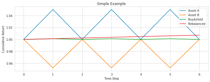

The code snippet is designed to create a plot illustrating the returns of two assets, A and B, with specific return values and a correlation coefficient of -1. The returns for assets A and B are provided as numpy arrays, with each array representing the returns of the respective assets in alternating years. The correlation coefficient of -1 indicates a perfect negative linear relationship between the two assets, meaning that when one asset’s return increases, the other’s return decreases proportionally.

Likely, the code uses a function called plot_simple_example (not provided in the snippet) to generate a plot based on the given returns and correlation coefficient. This function might plot the returns of assets A and B over time, highlighting their relative movements due to the negative correlation. The plot is saved as an SVG file named ‘Simple Example 3.svg’, which is a scalable vector graphic format that can be resized without loss of image quality.

The primary purpose of this code is to demonstrate the behavior of two assets with a perfect negative correlation in terms of their returns. By plotting their returns over multiple periods, the code visually depicts the inverse movement pattern between the assets. This type of analysis is valuable for portfolio diversification and risk management strategies, helping to visualize the relationship between the returns of assets A and B in a straightforward scenario where they exhibit perfect negative correlation.

Plotting a simple example of returns

# Asset A and B returns both have arith.mean 1 and correlation -1
plot_simple_example(returns_a=np.tile([1.05, 0.95], 3),
                    returns_b=np.tile([0.95, 1.05], 3),
                    filename='Simple Example 4.svg');

The code snippet appears to create a simple plot to demonstrate the concept of asset returns. For Asset A, returns alternate between 1.05 and 0.95, repeating this pattern three times. Similarly, Asset B’s returns alternate between 0.95 and 1.05, also repeating three times. By using these returns as input and specifying the filename for the plot, the function plot_simple_example likely generates a visual representation of how the returns of Assets A and B change, particularly illustrating their correlation. In this case, the assets have a correlation of -1, meaning their returns move in opposite directions.

This visual representation can help users understand the relationship between the returns of two assets. It showcases how changes in the return of one asset can affect the other, which is valuable for analyzing the risk and diversification benefits when holding multiple assets in a portfolio. Overall, this plot serves as an educational tool to grasp the interplay between the returns of different assets under varying conditions.

Plots number of available stocks

# Plot the number of available stocks with daily-returns.
plot_num_stocks(returns=daily_returns, returns_name=DAILY_RETURNS);

The code likely plots the number of available stocks that have daily returns using a function called plot_num_stocks. This function takes two arguments: returns, which appears to be the daily returns data, and returns_name, which might serve as the label for this data. The function presumably reads the daily returns data, counts the number of available stocks for each day, and then generates a plot to show how the number of available stocks changes over time based on their daily returns.

This code could be useful for analyzing the distribution of available stocks over time based on daily returns. It may assist in visualizing the relationship between the number of stocks and their returns, identifying patterns, or understanding the behavior of stocks in terms of availability and return rates.

Plot normalized and cumulative stock returns

# Plot the normalized and cumulative returns of all stocks.
plot_all_stock_traces(returns=daily_returns,
                      returns_name=DAILY_RETURNS, logy=True);

This code calls a function named plot_all_stock_traces to plot the normalized and cumulative returns of all stocks in a dataset called daily_returns. The returns_name parameter specifies the name of the returns, in this instance, as DAILY_RETURNS. The logy parameter is set to True, meaning the y-axis of the plot will be displayed on a logarithmic scale.

The function likely processes the dataset of returns (daily_returns), first normalizing the returns to start at the same point — usually 1 — to enable meaningful comparisons. It then calculates the cumulative returns and plots these normalized and cumulative returns on a graph. Using a logarithmic scale for the y-axis is beneficial when dealing with a wide range of values in financial data, as it allows for better visualization.

This code is particularly useful for analysts and investors as it enables the comparison of the performance of different stocks over time. By visualizing trends, patterns, and relative performances in a normalized and cumulative manner, it aids in understanding how different stocks have evolved and performed within a portfolio or market.

Simulate and plot random stock portfolios

# Simulate and plot pandom portfolios with 5 stocks each.
sim_plot_portfolio_traces(returns=daily_returns,
                          returns_name=DAILY_RETURNS,
                          num_stocks=5, num_trials=1000,
                          random_weights=False);

The code simulates and plots random portfolios composed of five stocks each using historical daily returns data stored in the variable daily_returns. By setting num_stocks to five, it specifies that each simulated portfolio will contain five randomly selected stocks. The num_trials parameter, set to 1000, indicates that 1000 different random portfolios will be generated and analyzed. Since random_weights is set to false, the portfolios will not have random weights assigned to each stock, likely meaning that equal weights will be used.

Overall, this code helps generate and visualize random portfolios, aiding investors or analysts in understanding the potential performance, risk, and diversification effects of different stock combinations. Visualizing multiple random portfolios provides insights into the range of potential outcomes, which is crucial for making informed investment decisions.

Simulate and plot 1000 portfolios

# Simulate and plot pandom portfolios with 50 stocks each.
sim_plot_portfolio_traces(returns=daily_returns,
                          returns_name=DAILY_RETURNS,
                          num_stocks=50, num_trials=1000,
                          random_weights=False);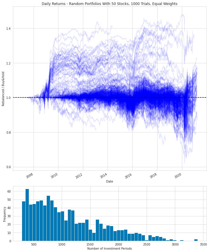

This code snippet simulates and plots the performance of random portfolios, each consisting of 50 different stocks. The key parameters include historical daily returns data of various stocks, possibly labeled as DAILY_RETURNS. Each portfolio comprises 50 stocks, and the analysis involves generating and examining 1000 random portfolios. The portfolios are not generated with random weights; instead, equal weights may be applied to each stock for simplicity or comparative analysis.

By calculating the performance of 1000 portfolios created from 50 stocks without random weights, the code facilitates portfolio analysis, evaluates diversification strategies, and studies the performance variability of randomly selected stock portfolios. This approach aids in understanding how different combinations of stocks influence overall portfolio performance and supports informed investment decisions.

Simulate and plot 100-stock portfolios

# Simulate and plot pandom portfolios with 100 stocks each.
sim_plot_portfolio_traces(returns=daily_returns,
                          returns_name=DAILY_RETURNS,
                          num_stocks=100, num_trials=1000,
                          random_weights=False);

This code is designed to simulate and plot portfolios comprising 100 different stocks, utilizing their historical daily returns provided in the daily_returns variable. The number of times the simulation will be run is determined by the num_trials parameter, with each trial using a different randomized selection of stocks. The random_weights parameter, when set to False, indicates that the portfolios will likely have equal weights assigned to each stock, rather than random weights.

The primary objective of this code is to analyze the performance of different 100-stock portfolios under various market conditions and visualize the results. This analysis aims to provide insights into portfolio diversification and risk management. By running the simulation multiple times, we can observe the range of possible outcomes and assess the variability in portfolio performance.

Simulate and plot random portfolios

# Simulate and plot pandom portfolios with 100 stocks each.
# NOTE: This uses random weights instead of equal weights.
sim_plot_portfolio_traces(returns=daily_returns,
                          returns_name=DAILY_RETURNS,
                          num_stocks=100, num_trials=1000,
                          random_weights=True);

The given code employs a function named sim_plot_portfolio_traces to simulate and plot portfolios comprised of 100 stocks each. It begins by taking daily returns data (daily_returns) as input to simulate these portfolios. The parameter returns_name designates the name of this returns data, which in this instance is DAILY_RETURNS. The portfolios are designed to include 100 stocks each, as specified by the num_stocks argument, and the simulations are executed 1000 times to explore various random configurations of the portfolios, as indicated by the num_trials parameter. With the random_weights parameter set to True, the function applies random weights to the stocks within each portfolio, meaning the allocation of funds to each stock is determined randomly.

The core idea behind this code is to analyze the performance and variability of portfolios assembled with random weights. Such simulations are invaluable for understanding the spectrum of potential outcomes arising from different portfolio configurations. By running numerous simulations, the code facilitates an assessment of the distribution of returns and associated risks linked with randomly assembled portfolios. This comprehensive analysis assists in making well-informed decisions about portfolio construction, asset allocation, and strategies for managing risk.

Simulates random portfolios and compares statistics

%%time
# Simulate random portfolios and plot all the statistics
# for comparing the Rebalanced and Buy&Hold portfolios.
sim_plot_compare_all(returns=daily_returns,
                     returns_name=DAILY_RETURNS,
                     num_stocks=num_stocks, num_trials=1000, 
                     random_weights=False,
                     pullup_window=int(BDAYS_PER_YEAR))

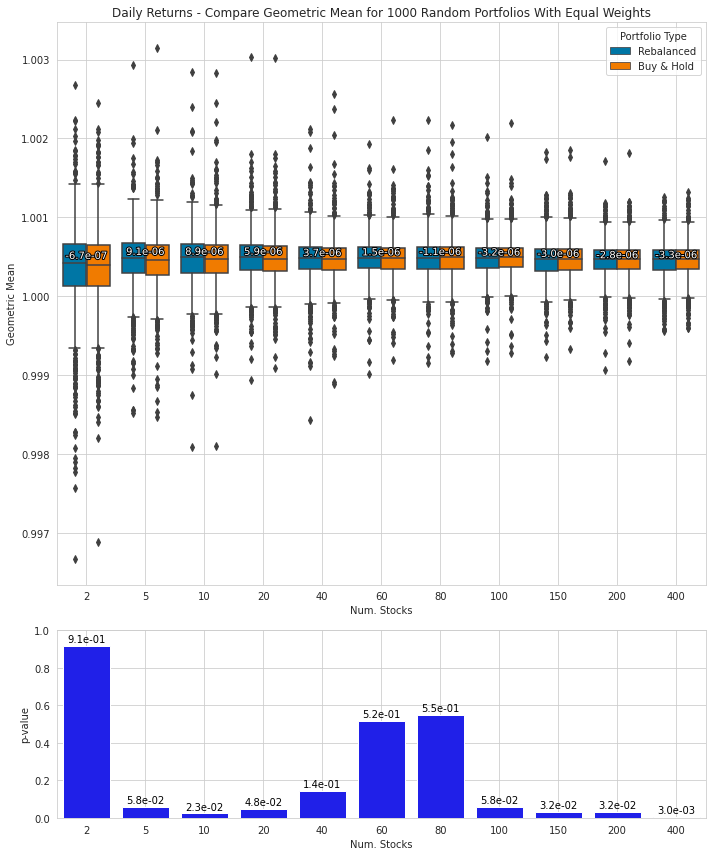
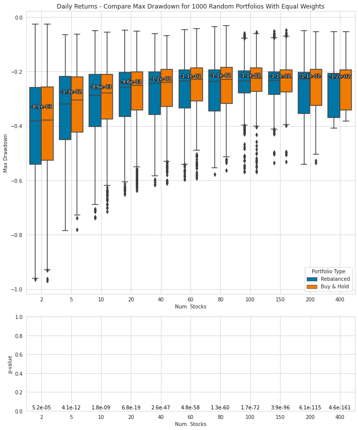
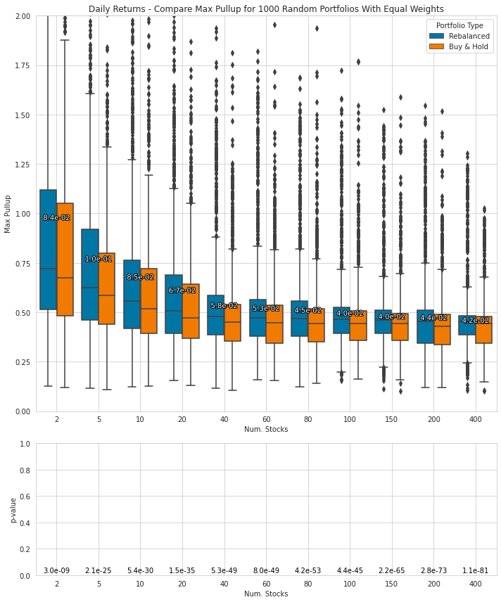
The code snippet provided conducts a simulation to evaluate the performance of two portfolio strategies: Rebalanced and Buy & Hold. Using daily returns data, it simulates random portfolios, then calculates and plots various statistics to compare the two strategies. Critical parameters in the simulation include the daily returns data, the number of stocks in the portfolio, the number of trials run, the application of random weights for the portfolios, and a pull-up window for calculation purposes.

The function sim_plot_compare_all likely computes and contrasts statistics such as portfolio returns, volatility, Sharpe ratio, drawdowns, and other performance metrics for the Rebalanced and Buy & Hold strategies. This dual analysis enables investors or analysts to visually and quantitatively determine which strategy offers superior risk and return profiles.

Such simulations and analyses aid investors in making informed decisions about the portfolio strategy that best suits their investment aims, risk tolerance, and time horizon. They also facilitate an understanding of potential outcomes and performance variations that could emanate from different investment strategies.

Simulate and compare random portfolios