


Enhancing Financial Forecasting with Advanced Deep Learning Techniques
Enhancing Financial Forecasting with Advanced Deep Learning Techniques
A Comparative Analysis of GRU, LSTM, and Baseline Models for Stock Market Predictions

Download the code using the link at the end of this article or in the comment section.
In the rapidly evolving landscape of financial markets, accurate forecasting remains a cornerstone for investors and analysts alike. This article delves into the cutting-edge realm of deep learning, showcasing the application of Gated Recurrent Unit (GRU) and Long Short-Term Memory (LSTM) models — two sophisticated neural network architectures renowned for their efficacy in handling time series data. Through a meticulous examination and implementation, we explore their performance in predicting stock market trends, juxtaposed against a baseline prediction model for benchmarking purposes.
The journey begins with a comprehensive setup involving essential Python libraries for data manipulation, scaling, and model building, including yfinance for fetching financial data, TensorFlow for constructing neural network models, and scikit-learn for preprocessing and metrics evaluation. A custom DataLoader class is introduced to efficiently manage financial time-series data, facilitating the creation of lagged features and normalization essential for neural network inputs.
As we progress, the focus shifts to the intricate process of building, training, and evaluating GRU and LSTM models, highlighting their unique capabilities in capturing temporal dependencies within stock price movements. The narrative further enriches with the integration of SHAP (SHapley Additive exPlanations) and LIME (Local Interpretable Model-agnostic Explanations) for model interpretability, offering insights into the driving factors behind the predictions.
Concluding with a visual comparison of actual versus predicted stock prices, this article offers a compelling narrative on the potential of GRU and LSTM models to revolutionize financial forecasting, providing a beacon for future explorations in the intersection of finance and artificial intelligence.
import yfinance as yf
import shap
import tensorflow as tf
import numpy as np
import pandas as pd
from sklearn.preprocessing import MinMaxScaler
from tensorflow.keras.models import Sequential
# Bidirectional ,
from tensorflow.keras.layers import Dense, LSTM,GRU, Reshape# captum (biblioteca de interpretação pytorch)
import matplotlib.pyplot as plt
from sklearn.metrics import mean_squared_error, mean_absolute_percentage_error, mean_absolute_error
from sklearn.base import BaseEstimator, TransformerMixin
tf.compat.v1.disable_v2_behavior() # caracteristica necessaria para o uso shap
This code snippet imports various Python libraries and performs some configurations that are typically used in machine learning and data analysis tasks involving neural networks and financial data. The library yfinance is imported to access financial data, likely for downloading stock market data such as historical stock prices. The shap library is a machine learning explainability tool used to understand the output of models. tensorflow is a deep learning framework used for building neural networks, and here it seems to be configured to use TensorFlow 1.x behavior with tf.compat.v1.disable_v2_behavior(), which is necessary for compatibility with the shap library at the time of writing.
The script also imports numpy and pandas, which are fundamental libraries for numerical computing and data manipulation in Python, respectively. MinMaxScaler from sklearn.preprocessing is typically used to scale input features to a neural network. For building the neural network, the script imports Sequential from tensorflow.keras.models, which is used to define a linear stack of layers for the neural network. It also imports various layer types from tensorflow.keras.layers, including Dense (fully connected layers), LSTM (long short-term memory units), and GRU (gated recurrent units), which are commonly used in recurrent neural networks (RNNs) for sequence data such as time series.
Additionally, matplotlib.pyplot is imported for plotting, which likely means that visualizations of the data or the models performance are intended. Lastly, it imports several metrics from sklearn.metrics, such as mean_squared_error, mean_absolute_percentage_error, and mean_absolute_error, which are used to evaluate the performance of regression models.
class DataLoader(BaseEstimator, TransformerMixin):
  def __init__(self, dataset: pd.DataFrame, lag):
    super()
    self.dataset = dataset
    self.dataset["Date"] = self.dataset["Date"].apply(lambda date: pd.to_datetime(date, format="ISO8601"))#,inplace=True

    self.lag = lag
    self.scaler = MinMaxScaler()

  def get_indexs_split(self, percent = .8):
    train_size = int(len(self.dataset) * percent)
    train_idx, test_idx = self.dataset.iloc[self.lag:train_size,:], self.dataset.iloc[train_size:,:]
    return train_idx.index, test_idx.index

  def fit(self, indexs, y=None):

    x_train = self.dataset[["Close"]].iloc[indexs]
    self.scaler.fit(x_train, [])
    return self

  def get_values(self):
     return self.values if self.values is not None else None

  def get_target(self):
     return self.target if self.target is not None else None

  def transform(self, indexs, y=None):
    if (indexs[0] - self.lag > 0):
       idxs = self.dataset.index[indexs[0] - (self.lag + 1): indexs[-1]]
    else:
       idxs = indexs

    X = self.dataset.loc[idxs]
    X.set_index(idxs)
    # landslides['date_parsed'] = pd.to_datetime(landslides['date'], format="%m/%d/%y")


    lagged_X = X[['Close']].copy()

    for lag in range(1, self.lag + 1):
        lagged_X[f'lag{lag}'] = lagged_X['Close'].shift(lag)
    lagged_X = lagged_X.apply(lambda x: (x-self.scaler.min_[0])/(self.scaler.data_max_[0] - self.scaler.min_[0]))
    # lagged_X = lagged_X.apply(lambda x: self.scaler.transform(x.reshape((1,-1))))

    lagged_X.dropna(inplace=True)
    self.values = lagged_X.drop(columns=['Close']).copy()
    self.target = lagged_X[['Close']].copy()

    return (np.array(lagged_X.drop(columns=['Close']).to_numpy(dtype=np.float32)),
            np.array(lagged_X[['Close']].to_numpy(dtype=np.float32)))

  def inverse_transform(self, X, y=None):
    # x_inverse = X.apply(lambda x: x*(self.scaler.data_max_[0] - self.scaler.min_[0]) + self.scaler.min_[0])
    x_inverse = np.apply_along_axis(lambda x: x*(self.scaler.data_max_[0] - self.scaler.min_[0]) + self.scaler.min_[0], 0, X)


    # x_inverse = X.apply(lambda x: self.scaler.inverse_transform(x), 0)
    #  self.scaler.inverse_transform(X)
    return x_inverse

  def fit_transform(self, X, y = None):
      return self.fit(X, y).transform(X, y)
This code defines a Python class named DataLoader which is intended to be used for loading and transforming financial time-series data, particularly for machine learning purposes. The class inherits from BaseEstimator and TransformerMixin, suggesting its compatibility with scikit-learns workflow, such as pipelines. Upon initialization, the DataLoader receives a pandas DataFrame dataset and an integer lag. It then converts the Date column of the dataset to datetime objects, assuming an ISO8601 date format. Additionally, it initializes a MinMaxScaler instance to scale the data. The get_indexs_split method is designed to split the dataset into training and testing indices based on a given percentage, percent, for the training size. By default, 80% of the data is intended for training. The fit method fits the MinMaxScaler to the Close prices in the dataset based on the provided indices, preparing the scaler for normalizing the data. The transform method applies a transformation to the dataset to create lagged features.
For each data point, it computes a set of new features that represent the Close prices from previous time steps (the lag). It then scales these features using the previously fitted MinMaxScaler and returns both the lagged features and the associated target values in the form of numpy arrays. The inverse_transform method reverses the scaling operation, converting scaled data back to its original range, which is useful for interpreting model predictions. Lastly, the fit_transform method is a convenience that combines the fit and transform operations, typical for sklearn transformers. All in all, the DataLoader class is designed to preprocess financial time-series data by creating lagged features and normalizing them, so as to facilitate the development of machine learning models for tasks such as forecasting.
data = pd.read_csv("../data.csv")
data = data[["Date", "Close"]]
This code performs two main operations related to handling data using the pandas library in Python. Firstly, pd.read_csv(../data.csv) is used to read the content of a CSV file named data.csv which is located in the parent directory of the current working directory (as indicated by the path ../data.csv). The pd.read_csv function is a common way to import data from a CSV file into a DataFrame, which is a two-dimensional, size-mutable, and potentially heterogeneous tabular data structure with labeled axes (rows and columns) provided by the pandas library. After reading the CSV file into a DataFrame and assigning it to the variable data, the second operation data = data[[Date, Close]] is a selection operation that filters the columns of the DataFrame. It reduces the DataFrame to only include the columns Date and Close. By doing this, all other columns that might be present in the original CSV file are discarded, and data is updated to contain just these two specified columns. This is typically done to focus on the data that is relevant for further analysis or processing, such as time series analysis on financial closing prices where only the date and closing price columns are required.
Normalize
data_loader = DataLoader(data, lag=6)
train_indexs, test_indexs = data_loader.get_indexs_split()
x_train, y_train = data_loader.fit_transform(train_indexs)
The snippet is creating a DataLoader object with some dataset data and a lag parameter set to 6. The DataLoader is assumed to be a custom class designed to handle the loading and preprocessing of the data for a time series or sequence prediction task. The lag parameter of 6 implies that the DataLoader might use this value to create features based on the lagged observations, which is a common approach in time-series forecasting where past values are used to predict future ones.
After initializing the data loader, the code proceeds to split the data into training and testing sets by calling the get_indexs_split() method on the DataLoader object. This method probably returns the indices for the train and test datasets. These indices are stored in train_indexs and test_indexs variables. Following the index split, the code segment fetches the training data (x_train and y_train) by applying fit_transform on the train_indexs. This indicates that fit_transform method of the DataLoader is used for preprocessing the data corresponding to the training indices, likely scaling the features (x_train) and perhaps encoding the target variable (y_train) if necessary. The preprocessed training features and labels are then ready to be used by a machine learning model for training.
x_train.shape, y_train.shape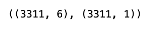
This code is a expression that is likely used to retrieve the dimensions, or shapes, of two variables: x_train and y_train. These variables are commonly used to represent the feature set and the labels, respectively, in a machine learning context. x_train typically contains the input data that will be used to train a model, and y_train contains the corresponding target outputs or labels. When this code is executed, it will return a tuple with the shapes of x_train and y_train. The shape of an array or a data structure in Python (often a NumPy array or a pandas DataFrame when dealing with machine learning datasets) tells you how many elements there are along each axis. For example, in a 2D array, the shape will tell you the number of rows and columns. This information is useful for verifying that the data is correctly formatted before it is fed into a machine learning algorithm for training. It can help in debugging issues related to dimensionality mismatches and is often an important step in the data pre-processing phase.
x_train[0], y_train[0]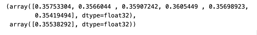
The purpose of this code is to access the first element of two arrays (or other indexed collections such as lists), specifically x_train and y_train. These names usually indicate that they are the training data and labels used in a machine learning context. The x_train array likely contains the features or input variables, while the y_train array contains the corresponding targets or output labels. By accessing the first element of each (x_train[0] for the first feature vector and y_train[0] for the first target label), it suggests that we might be examining or processing the first training example in a dataset.
tf.random.set_seed(22)This line of code is used to set a seed for random number generation in TensorFlow, which is a machine learning and numerical computation library. The purpose of setting a seed with the value 22 is to ensure that the operations which rely on random number generation can be reproduced exactly. This is important when you want to have deterministic behavior in stochastic processes, such as when you initialize weights in a neural network or when you shuffle data for training. By using the same seed, you ensure that each time the code is run, even on different machines or at different times, the random numbers generated are the same, which is helpful for debugging and for comparing the results of different runs or models.
# Define the GRU model
def GRU_Model(output_window, look_back):
    model = Sequential([
            tf.keras.layers.Reshape((1, -1)),
            tf.keras.layers.GRU(128, return_sequences=False, input_shape=(1, look_back)),
            tf.keras.layers.Dense(output_window)
        ])
    # optimizer = tf.keras.optimizers.Adam(learning_rate=1e-4)
    # model.compile(optimizer=optimizer , loss='mean_squared_error')
    model.compile(optimizer="adam" , loss='mean_squared_error')
    return model

# Define the LSTM model
def LSTM_Model(output_window, look_back):
    model = Sequential([
        tf.keras.layers.Reshape((1, -1)),
        tf.keras.layers.Bidirectional(
            tf.keras.layers.LSTM(128, activation='relu', input_shape=(1, look_back), return_sequences=True)),
        tf.keras.layers.Dense(output_window)
    ])
    model.compile(optimizer="adam" , loss='mean_squared_error')

    return model

# Define the baseline model
def baseline_model(output_window, y_train):
    last_known_value = y_train[-1]
    return np.full((len(y_test), output_window), last_known_value)

# Train and evaluate the models
output_window = 1
gru_model = GRU_Model(output_window, data_loader.lag)
lstm_model = LSTM_Model(output_window, data_loader.lag)
The code snippet defines three different predictive models: A GRU model, an LSTM model, and a baseline model, which are likely to be used for time-series forecasting or sequence prediction tasks. The first function GRU_Model creates a Gated Recurrent Unit (GRU) model with 128 GRU units and expects input data with a feature window specified by look_back. The output_window parameter indicates the dimension of the models output layer, which is a Dense layer. The model is compiled with the Adam optimizer and uses mean squared error as the loss function.
The second function LSTM_Model creates a model with a Bi-directional Long Short-Term Memory (LSTM) layer. This implies the model processes the sequence data in both directions (forward and backward), potentially improving its context understanding for forecasting. It also features 128 LSTM units and employs an output Dense layer tailored by output_window. The ReLU activation function is specified for the LSTM units, and similarly to the GRU model, its compiled using Adam and mean squared error.