

Ensemble Methods Advanced concepts
A step by step guide.

import addutils.toc ; addutils.toc.js(ipy_notebook=True)This code imports a module named addutils.toc that likely includes a function js() to add a table of contents (TOC) to an iPython (Jupyter) notebook. The function js() seems to generate a dynamic TOC for the cells in the notebook, allowing for easier navigation within the notebook content. By providing the argument ipy_notebook=True, the function is likely configured to work specifically with Jupyter notebooks. The purpose of adding a TOC to a notebook is to improve the readability and navigation experience for users who want to quickly find and access specific sections or content within the notebook without having to scroll through the entire document.
There is no source code for this article.
import scipy.io
import numpy as np
import pandas as pd
from time import time
from sklearn import model_selection, metrics, ensemble, datasets
import arff
from addutils import css_notebook
import sys
import os
import warnings
css_notebook()
This code snippet imports various libraries and modules that are commonly used in data analysis and machine learning tasks. The scipy.io library is imported for input/output operations, numpy for numerical operations and array handling, pandas for data manipulation and analysis, and time for time-related functionalities. The sklearn library is imported for machine learning algorithms, such as model selection, metrics, and ensemble techniques. The datasets module is imported from sklearn to access built-in datasets. Additionally, the code imports arff for working with Attribute-Relation File Format (ARFF) files, and addutils for additional utility functions. Finally, sys, os, and warnings are imported for system-related operations and handling warnings. The css_notebook() function from addutils is called to apply custom styling to the Jupyter notebook environment. Overall, this code sets up the necessary libraries and utilities for data analysis and machine learning tasks within a Jupyter notebook.
import bokeh.plotting as bk
bk.output_notebook()
Loading BokehJS …
This code snippet uses the Bokeh library to generate interactive data visualizations in a Jupyter notebook. The import bokeh.plotting as bk line imports the necessary functionalities from the Bokeh library, allowing the creation of plots like scatter plots, line plots, and bar charts. The bk.output_notebook() function call is used to display the interactive Bokeh plots directly within the Jupyter notebook environment. By invoking this function, the resulting plots will be rendered inline in the notebook, providing an interactive and visually appealing way to explore and analyze data.
Introduction
In this notebook we introduce some advanced techniques that can be used effectively with ensemble methods:
OOB Score (Estimates)
Feature Importance
Partial Dependece Plot
Out of Bag Estimates
When using ensemble methods based upon Bootstrap aggregation or Bagging, i.e. using sampling with replacement, a part of the training set remains unused. For each classifier in the ensemble, a different part of the training set is left out. This left out portion can be used to estimate the generalization error without having to rely on a separate Validation Set. This estimate comes “for free” as no additional data is needed and can be used for model selection or for tuning hyperparameter.
This is currently implemented in the following classes:
RandomForestClassifier / RandomForestRegressor
ExtraTreesClassifier / ExtraTreesRegressor
GradientBoostingClassifier / GradientBoostingRegressor
Remarks
In GradientBoosting OOB score is available only when subsample $< 1.0$. It can be used for a different purpose, that is finding the optimal number of boosting iterations, but it is a pessimistic estimator of the true test error. Use it only for saving computataional time since, for example, cross-validation is more demanding.
Phishing Websites Data Set
For testing OOB Score properties of ensemble method we used a publicly available dataset. The dataset is the Phishing Websites Data Set and can be downloaded from here. This dataset is anonymized by replacing the actual strings with describing values.
The dataset is available in Weka format, so we have to use the Weka arff file type reader for python to read it.
#load the dataset
with open('example_data/Training Dataset.arff', 'rb') as f:
    file_ = f.read().decode('utf-8')
f.close()
#print(file_)
data = arff.load(file_)
print("Keys: ")
for k in data.keys():
    print("- " + k)
Keys:
- description
- relation
- attributes
- dataThis code snippet loads a dataset from a file in ARFF (Attribute-Relation File Format), which is a common format for representing machine learning datasets. It reads the content of the file Training Dataset.arff, decodes it using the UTF-8 encoding scheme, and then loads the data into a dictionary using the arff.load function. After loading the dataset, the code prints out the keys of the dictionary, which typically represent different components of the dataset such as the data instances, attribute information, and metadata. The loop iterates over the keys in the dictionary and prints them with a prefix of a dash (-) to display the keys in a formatted way. This helps in understanding the structure and contents of the dataset after loading it from the ARFF file.
In attributes are stored the column names while actual data is stored in data. The dataset is further divided into training and test set to compare OOB score with CV and held out set.
#use the dataset to build a dataframe
cols = [at[0] for at in data['attributes']]
df = pd.DataFrame(data['data'], dtype=int, columns=cols)
print("Shape of the data: {0}".format(df.shape))
target = df.iloc[:,-1]
train = df.iloc[:,:-1]
#split the dataframe in train / test
X_train, X_test, y_train, y_test = model_selection.train_test_split(train,
                                                                     target,
                                                                     test_size=0.2)
print("Training set / Test set number of samples: {0}, {1}".format(X_train.shape[0],
                                                                   X_test.shape[0]))
print("Number of features: {0}".format(X_train.shape[1]))
Shape of the data: (11055, 31)
Training set / Test set number of samples: 8844, 2211
Number of features: 30This code snippet reads a dataset, which is assumed to be in a dictionary format containing attributes and data. It first creates a DataFrame df using the attributes from the dataset and the data values. It then splits this DataFrame into the target variable (last column) and the training data (everything except the last column). It splits this data into training and testing sets using an 80/20 ratio. The code then prints the shapes of the training and testing sets, as well as the number of features in the training set. This process sets up the data for further analysis or machine learning model training.
pd.options.display.max_columns=6
df.head(3)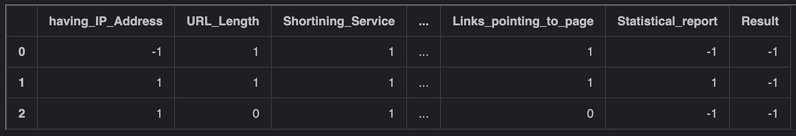
This code sets the maximum number of columns to display in the Pandas DataFrame to 6. The pd.options.display.max_columns attribute is used to adjust the display settings for Pandas DataFrames. By changing this attribute to 6, it ensures that only up to 6 columns will be shown when displaying the DataFrame. Subsequently, df.head(3) is used to display the first 3 rows of the DataFrame df. By combining these two commands, the code first sets the display option for the maximum number of columns and then displays the top 3 rows of the DataFrame with the updated display settings, showing only up to 6 columns for each of the rows. This is particularly useful when dealing with DataFrames that have a large number of columns, allowing for a more concise representation of data during output.
OOB estimate Random Forest
Test OOB score against cross-validation and test set. In order to perform OOB score calculation the option oob_score must be set to True.
t0 = time()
rfc = ensemble.RandomForestClassifier(n_estimators=1000,
                                      oob_score=True,
                                      random_state=42,
                                      n_jobs=-1)
rfc.fit(X_train, y_train)
print('RF fit done in %0.3f[s]' %(time() - t0))
t0 = time()
cv_score = model_selection.cross_val_score(rfc, train, target, cv=10, n_jobs=-1)
print('CV score calculated in %0.3f[s]' %(time() - t0))
RF fit done in 2.194[s]
CV score calculated in 8.276[s]This code snippet uses scikit-learn library to train a Random Forest Classifier model using the RandomForestClassifier class. The model is trained on the training data X_train with labels y_train. The RandomForestClassifier is configured with 1000 decision trees (n_estimators=1000), calculates out-of-bag estimation score (oob_score=True), and uses 42 as the random seed (random_state=42). The training is done in parallel using all available cores (n_jobs=-1). After training the model, it then performs k-fold cross-validation to evaluate the models performance using the cross_val_score function from the model_selection module. Here, the cross-validation is performed with 10 folds (cv=10) and in parallel using all available cores (n_jobs=-1). The cross-validation scores are stored in the variable cv_score. Finally, the code prints the time taken for fitting the Random Forest model and calculating the cross-validation score by measuring the time before and after each operation using the time function from the time module, and then calculating the difference. The timing information is printed to the console to provide insights into the computational cost of these operations.
As can be seen in this example, using CV to measure the score takes time and it is similar to that obtained from OOB samples, that comes with the algorithm at no additional computational costs.
print('Score comparison:')
print('F1 score (on the test set):'.ljust(40), '%f' % metrics.f1_score(rfc.predict(X_test),\
                                                                       y_test))
print('OOB score:'.ljust(40), '%f' % rfc.oob_score_)
print('CV score (on the entire training set):'.ljust(40), '%f' % cv_score.mean())
Score comparison:
F1 score (on the test set): 0.974850
OOB score: 0.970828
CV score (on the entire training set): 0.972767This code is intended to display a comparison of different scores related to a classification model. The print statements show the F1 score on the test set, the Out-of-Bag (OOB) score, and the cross-validated (CV) score on the entire training set. The .ljust(40) method is used to align the score description with a fixed width of 40 characters for better readability. The %f formatting is used to display the numerical score values, with the scores retrieved from the metrics module. Specifically, the F1 score is calculated using the f1_score function, the OOB score is obtained directly from the random forest classifier (rfc), and the CV score is calculated as the mean of the cross-validated scores (cv_score). Overall, the code provides a clear and formatted output of different evaluation scores for the classification model.
OOB estimate Gradient Boosting
Please be patient: the following cell will require up to 10 minutes to be computed
# Fit classifier with out-of-bag estimates
params = {'n_estimators': 11000,
          'max_depth': 3,
          'subsample': 0.5,
          'learning_rate': 0.1,
          'min_samples_leaf': 1,
          'random_state': 3}
clf = ensemble.GradientBoostingClassifier(**params)
t0 = time()
clf.fit(X_train, y_train)
print('GBRT fit done in %0.3f[s]' %(time() - t0))
acc = clf.score(X_test, y_test)
print("Accuracy: {:.4f}".format(acc))
n_estimators = params['n_estimators']
x = np.arange(n_estimators) + 1
def heldout_score(clf, X_test, y_test):
    """compute deviance scores on ``X_test`` and ``y_test``. """
    score = np.zeros((n_estimators,), dtype=np.float64)
    for i, y_pred in enumerate(clf.staged_decision_function(X_test)):
        score[i] = clf.loss_(y_test, y_pred)
    return score

def cv_estimate(n_folds=3):
    cv = model_selection.KFold(n_splits=n_folds, random_state=42)
    cv_clf = ensemble.GradientBoostingClassifier(**params)
    val_scores = np.zeros((n_estimators,), dtype=np.float64)
    for train, test in cv.split(X_train):
        cv_clf.fit(X_train.iloc[train], y_train.iloc[train])
        val_scores += heldout_score(cv_clf, X_train.iloc[test], y_train.iloc[test])
    val_scores /= n_folds
    return val_scores

# Estimate best n_estimator using cross-validation
t0 = time()
cv_score = cv_estimate(3)
print('CV score estimate done in %0.3f[s]' %(time() - t0))
# Compute best n_estimator for test data
test_score = heldout_score(clf, X_test, y_test)
# negative cumulative sum of oob improvements
cumsum = -np.cumsum(clf.oob_improvement_)
# min loss according to OOB
oob_best_iter = x[np.argmin(cumsum)]
# min loss according to test (normalize such that first loss is 0)
test_score -= test_score[0]
test_best_iter = x[np.argmin(test_score)]
# min loss according to cv (normalize such that first loss is 0)
cv_score -= cv_score[0]
cv_best_iter = x[np.argmin(cv_score)]
GBRT fit done in 79.233[s]
Accuracy: 0.9720
CV score estimate done in 168.519[s]This code is fitting a Gradient Boosting Classifier (GBRT) model using specified parameters and then evaluating its performance. The model is trained on the provided training data (X_train and y_train) with the specified parameters like the number of estimators, maximum depth, subsample ratio, learning rate, minimum samples leaf, and random state. The accuracy of the classifier is then calculated on the test data (X_test, y_test) using the score method. After fitting the model, the code defines a function heldout_score to compute deviance scores for the test data based on the staged decision function of the classifier. It then defines a cross-validation function using KFold and uses it to estimate the best number of estimators for the GBRT model. The code calculates the cross-validation score estimate and the best number of estimators using the cv_estimate function. Lastly, the code calculates the best number of estimators based on the out-of-bag (OOB) improvements, test data, and cross-validation scores. It computes the cumulative sum of OOB improvements and finds the iteration with the minimum loss for OOB, test data, and cross-validation. These values provide insights into the performance of the GBRT model with different numbers of estimators on various datasets.
As stated in the introduction OOB estimate for Gradient Boosting can be used for computing the optimal number of boosting itarations. It has the advantage of being computed on the fly as a byproduct of the algorithm, but it has the disadvantage of being a pessimistic estimate of the actual loss, especially for high number of trees. In the following picture the OOB loss estimate is plotted against test and CV score. The curves represent the cumulative sum of negative improvement as a function of the number of boosting iterations. The vertical line represent the point were the curve is lower.
from bokeh.models import LinearAxis, Range1d
oob_best_iter = int(oob_best_iter)
test_best_iter = int(test_best_iter)
cv_best_iter = int(cv_best_iter)
fig = bk.figure(plot_width=700, plot_height=500)
fig.line(x, cumsum, color="blue", legend="OOB loss")
fig.ray(x=oob_best_iter, y=0, length=0, angle=(np.pi / 2), line_width=1, color="blue")
fig.ray(x=oob_best_iter, y=0, length=0, angle=-(np.pi / 2), line_width=1, color="blue")
fig.text(x=oob_best_iter+100, y=-85, text=["OOB best"], text_font_size='8pt')
fig.line(x, test_score, color="red", legend="Test loss")
fig.ray(x=test_best_iter, y=0, length=0, angle=(np.pi / 2), line_width=1, color="red")
fig.ray(x=test_best_iter, y=0, length=0, angle=-(np.pi / 2), line_width=1, color="red")
fig.text(x=test_best_iter-900, y=-80, text=["Text best"], text_font_size='8pt')
fig.line(x, cv_score, color="green", legend="CV loss")
fig.ray(x=cv_best_iter, y=0, length=0, angle=(np.pi / 2), line_width=1, color="green")
fig.ray(x=cv_best_iter, y=0, length=0, angle=-(np.pi / 2), line_width=1, color="green")
fig.text(x=cv_best_iter-900, y=-85, text=["CV best"], text_font_size='8pt')
fig.xaxis.axis_label = "number of iterations"
fig.xaxis.axis_label_text_font_size = '10pt'
fig.yaxis.axis_label = "normalized loss"
fig.yaxis.axis_label_text_font_size = '10pt'
bk.show(fig)
This code utilizes the Bokeh library to create a plot visualizing the training progress of a model. The fig object is a figure where three lines are plotted: OOB loss in blue, Test loss in red, and CV loss in green. Each line represents the loss over the number of iterations. The code also includes markers to highlight the best iteration for OOB, Test, and CV losses. These markers are represented by vertical lines at the respective best iteration points along with a small text annotation mentioning the type of loss and indicating it as the best. These markers help in visually identifying the best performing iterations for the different loss calculations. Lastly, the plots x and y axes are labeled accordingly for clarity. Once all the elements are added to the plot, the bk.show(fig) command is used to display the plot in the output. Overall, this code creates a comprehensive visualization aiding in analyzing and comparing the performance of the model during training based on different loss metrics.
As we can see from the picture, the OOB score start increasing for a low number of iterations, while CV and Test loss continue decreasing. Use this feature only when performing Cross Validation overhead is unacceptable.
Ensemble Methods comparison
We can use this example to further compare Random Forest and Gradient Boosting Regression Trees.
Once xgboost is installed and working properly, the following cell should work automatically.
try:
    import xgboost as xgb
params = {'n_estimators': 11000,
              'max_depth': 3,
              'subsample': 0.5,
              'learning_rate': 0.1}
    xgb_model = xgb.XGBClassifier(**params)
    t0 = time()
    xgb_model.fit(X_train.values, y_train)
    print('XGBoost fit done in %0.3f[s]' %(time() - t0))
    xgb_acc = xgb_model.score(X_test.values, y_test)
    print("Accuracy: {:.4f}".format(xgb_acc))
except ModuleNotFoundError:
    print('If you want to use xgboost, install it first, following instructions!')
If you want to use xgboost, install it first, following instructions!This code first attempts to import the XGBoost library to use for training a model. It specifies some hyperparameters such as the number of estimators, maximum depth, subsample, and learning rate for the XGBoost classifier. The XGBoost classifier is then created with these hyperparameters. The code then measures the time taken to fit the XGBoost model on the training data and prints the time taken to complete the fitting process. After fitting, it calculates the accuracy of the XGBoost model on the test data and stores it in the variable xgb_acc. The accuracy is then printed out to the console with four decimal places. If the XGBoost library is not found (ModuleNotFoundError), it will print a message instructing the user to install XGBoost before using it for training a model.
