


Evaluating LSTM Predictions Against SPX Market Trends
Evaluating LSTM Predictions Against SPX Market Trends
Comparative Analysis of Automated Predictive Models and Market Indices

In the realm of financial analytics, leveraging advanced computational models like Long Short-Term Memory (LSTM) neural networks offers a sophisticated method to predict market movements. These models, when trained on historical data, can capture complex temporal patterns and dependencies, providing a predictive insight that is invaluable for traders, analysts, and investors alike. The S&P 500 Index (SPX), a market-capitalization-weighted index of the 500 largest U.S. publicly traded companies, serves as a primary benchmark for U.S. equity performance. By comparing the LSTM model’s predictions against the actual SPX values, analysts can evaluate the accuracy and efficacy of such predictive models in real-world scenarios.
The process begins with the meticulous preparation and segmentation of data, where historical SPX indices are divided into training and validation sets. This is crucial for training the LSTM model under conditions that closely mimic the unpredictable nature of financial markets. The model’s predictions, translated into a ‘Closing Price Bot’, are then juxtaposed with the actual ‘Closing Price’ movements of the SPX. This comparison not only highlights the model’s predictive capabilities but also sheds light on potential areas for improvement. By examining the differential performance between the model’s outputs and actual market trends, financial analysts can refine their strategies, adjust risk management protocols, and optimize investment portfolios for better returns.
Moreover, the analysis extends beyond mere prediction accuracy. It delves into the foundational aspects of financial time series analysis, such as trend identification, volatility assessment, and the impact of macroeconomic variables. This comprehensive approach ensures that predictive modeling is not just about forecasting numbers but understanding the underlying market dynamics that drive those numbers. Through iterative learning and model optimization, the goal is to enhance the predictive framework’s reliability, making it a potent tool in the arsenal of financial analysis and decision-making.
pip install stockstatsThe command pip install stockstats is not a code snippet but rather a command line instruction used to install a Python library called stockstats. When executed, the command performs the following steps: 1. It calls pip, which is the package installer for Python. Pip is used to install and manage software packages written in Python. 2. It invokes the install command of pip, which is responsible for installing packages from the Python Package Index (PyPI) or other indexes. 3. It specifies the name of the package to be installed, which in this case is stockstats. stockstats is a library designed to help with the statistical analysis of stock market data. Upon running this command, pip will contact PyPI, find the stockstats package, download it, and install it along with its dependencies into the Python environment being used. After installation, the stockstats library can be imported and used in Python code to work with stock data.
import pandas_datareader.data as web
import datetime as dt
from datetime import timedelta
import pandas as pd
import matplotlib.pyplot as plt
from statsmodels.graphics.tsaplots import plot_acf, plot_pacf
import numpy as np
import seaborn as sns
from stockstats import StockDataFrame as Sdf
import scipy
import pywt
from sklearn.metrics import confusion_matrix
import math
from pandas.tseries.offsets import CustomBusinessDay, DateOffset, WeekOfMonth
from pandas.tseries.holiday import sunday_to_monday, AbstractHolidayCalendar, Holiday, USMemorialDay, USLaborDay, USColumbusDay, USThanksgivingDay
from sklearn import metrics
from rpy2.robjects import pandas2ri
import rpy2.robjects as objects
from statsmodels.tsa.api import VAR
from statsmodels.tsa.stattools import adfuller
from statsmodels.tools.eval_measures import rmse, aic
import warnings
warnings.filterwarnings('ignore')
print("pandas version %s" % pd.__version__)
The code is a Python script that starts by importing a variety of libraries used for data analysis, financial data retrieval, statistical analysis, and plotting. Heres a brief, step-by-step explanation of its purpose and functionalities:
It imports the pandas_datareader.data module as web to fetch financial market data from various internet sources.
It imports datetime libraries to work with dates and times.
The pandas library (as pd) is imported for data manipulation and analysis.
It imports the matplotlib.pyplot library as plt for creating static, animated, and interactive visualizations.
The statsmodels.graphics.tsaplots module is used for plotting autocorrelation function (ACF) and partial autocorrelation function (PACF) graphs, which are helpful for identifying patterns in time series data.
It imports the numpy library as np for numerical operations on arrays and matrices.
The seaborn library as sns is for making statistical graphics more attractive and informative.
The stockstats modules StockDataFrame is imported as Sdf for converting stock data into a pandas.DataFrame with useful indicators.
The scipy library is included for scientific and technical computing.
pywt is a library for wavelet transforms, which are used for time-frequency analysis of signals.
The sklearn.metrics module includes the confusion_matrix for evaluating the accuracy of a classification.
It imports math functions.
Several date offset classes from pandas.tseries.offsets are imported for custom date manipulation, particularly for business days.
Different US holiday related classes and functions are imported from pandas.tseries.holiday to adjust for holidays in time series analysis.
More sklearn metrics and tools are loaded.
The rpy2.robjects is imported for converting between pandas data frames and r data frames, as well as using R inside Python.
The vector autoregression (VAR) model from statsmodels.tsa.api is imported, possibly to conduct multivariate time series analysis.
The Augmented Dickey-Fuller test from statsmodels.tsa.stattools, which is a statistical test for checking the stationarity of a time series.
Functions for evaluating model performance (rmse, aic) are imported from statsmodels.tools.eval_measures.
Python warnings are set to be ignored which could suppress any warning messages. Lastly, the code prints the version of the pandas library to ensure the user knows which version is being used, implying compatibility or potential issues with utilized functions in different versions. This code seems to prepare the environment for a comprehensive financial and time series analysis, likely leading up to a predictive modeling task or exploratory data analysis with an emphasis on handling date and time efficiently and considering market-specific constraints and patterns.
sns.set(rc={'figure.figsize':(20, 7)})The code snippet is a command using Seaborn, a visualisation library in Python. This command is configuring the default figure size for the plots created by Seaborn. Specifically, it sets the figure width to 20 units and the height to 7 units. The rc parameter allows customization of the appearance of figures created with Seaborn by passing a dictionary of relevant Matplotlib properties. Here, the figure.figsize property is being set, which determines the size of figures drawn; larger figures can display more detail, while smaller figures take up less space on screen or in printed material. After this command, all Seaborn plots will be drawn with the specified figure size unless it is overridden in further plotting commands.
# Code to read csv file into Colaboratory:
from pydrive.auth import GoogleAuth
from pydrive.drive import GoogleDrive
from google.colab import auth
from oauth2client.client import GoogleCredentials
# Authenticate and create the PyDrive client
auth.authenticate_user()
gauth = GoogleAuth()
gauth.credentials = GoogleCredentials.get_application_default()
drive = GoogleDrive(gauth)
This code snippet is used to authenticate a user and set up the Google Drive client within a Google Colab environment, allowing the user to read CSV files from Google Drive into their Colab notebook. Step by step:
Import necessary libraries for authentication and Google Drive access.
Authenticate the user running the code within Google Colab using their Google account. This is facilitated by calling auth.authenticate_user() which opens a prompt for the user to log in.
Initialize a GoogleAuth object for further authorization processes.
Set the credentials of the GoogleAuth object to the default credentials obtained after the user authentication.
Create a GoogleDrive object passing the authenticated GoogleAuth object to it, which establishes the connection between the Colab environment and the users Google Drive. After executing this code, the users Colab notebook has access to read files from the users connected Google Drive.
# Load dataset from google drive
id = '1ATmaZrLwm1_hE1I1p7s2S1rjpLXv1ozx'
downloaded = drive.CreateFile({'id':id})
downloaded.GetContentFile('dataset.xlsx')
The snippet of code is used to download a specific file from Google Drive into a local environment, likely in a Jupyter Notebook or a similar Python environment that has access to Google Drive API via the PyDrive library. The code works as follows:
It specifies a Google Drive file ID, which uniquely identifies the file being accessed. This ID corresponds to a file named dataset.xlsx.
Then, it creates a Google Drive file object using the PyDrives CreateFile method with the given file ID.
After the file object is created, it calls the GetContentFile method on this object to download the file. As a result, dataset.xlsx is saved in the current working directory of the Python environment from which the code is run.
Preprocessing
df_BcBalance = pd.read_excel("dataset.xlsx", sheet_name = 'Bilan BC')
df_BcBalance.set_index('Date', inplace = True, drop = True)
df_BcBalance = df_BcBalance.resample('D').fillna(method = 'ffill')

df_daily_data = pd.read_excel("dataset.xlsx", sheet_name = 'Données journalières')
df_daily_data.set_index('Date', inplace = True, drop = True)
del df_daily_data['CRB - Bétail']

df_EconomicalSurprise = pd.read_excel("dataset.xlsx", sheet_name = 'Surprise économique')
df_EconomicalSurprise.set_index('Date', inplace = True, drop = True)
df_EconomicalSurprise = df_EconomicalSurprise.resample('D').fillna(method = 'ffill')

df_FedBalance = pd.read_excel("dataset.xlsx", sheet_name = 'Bilan FED')
df_FedBalance.set_index('Date', inplace = True, drop = True)
df_FedBalance = df_FedBalance.resample('D').fillna(method = 'ffill')

df_gold = pd.read_excel("dataset.xlsx", sheet_name = 'Or')
df_gold.set_index('Date', inplace = True, drop = True)
df_gold = df_gold.resample('D').fillna(method = 'ffill')

df_InflationUnemployment = pd.read_excel("dataset.xlsx", sheet_name = 'Chômage & Inflation')
df_InflationUnemployment.set_index('Date', inplace = True, drop = True)
df_InflationUnemployment = df_InflationUnemployment.resample('D').fillna(method = 'ffill')

df_oil = pd.read_excel("dataset.xlsx", sheet_name = 'Pétrole')
df_oil.set_index('Date', inplace = True, drop = True)
df_oil = df_oil.resample('D').fillna(method = 'ffill')

df_ProductionCapacity = pd.read_excel("dataset.xlsx", sheet_name = 'Capacité de production')
df_ProductionCapacity.set_index('Date', inplace = True, drop = True)
df_ProductionCapacity = df_ProductionCapacity.resample('D').fillna(method = 'ffill')

df_SPX = pd.DataFrame(df_daily_data['SPX Index'].copy())
df_SPX.index = df_daily_data.index.copy()
#del df_daily_data['SPX Index']

df_daily_data = df_daily_data.join(df_BcBalance).join(df_EconomicalSurprise).join(df_gold).join(df_InflationUnemployment).join(df_ProductionCapacity)
df_daily_data = df_daily_data[(df_daily_data.index >= '2000-12-31') & (df_daily_data.index <= '2019-12-31')]

df_SPX = pd.DataFrame(df_daily_data['SPX Index'].copy())
df_SPX.index = df_daily_data.index.copy()
df_daily_data.head(10)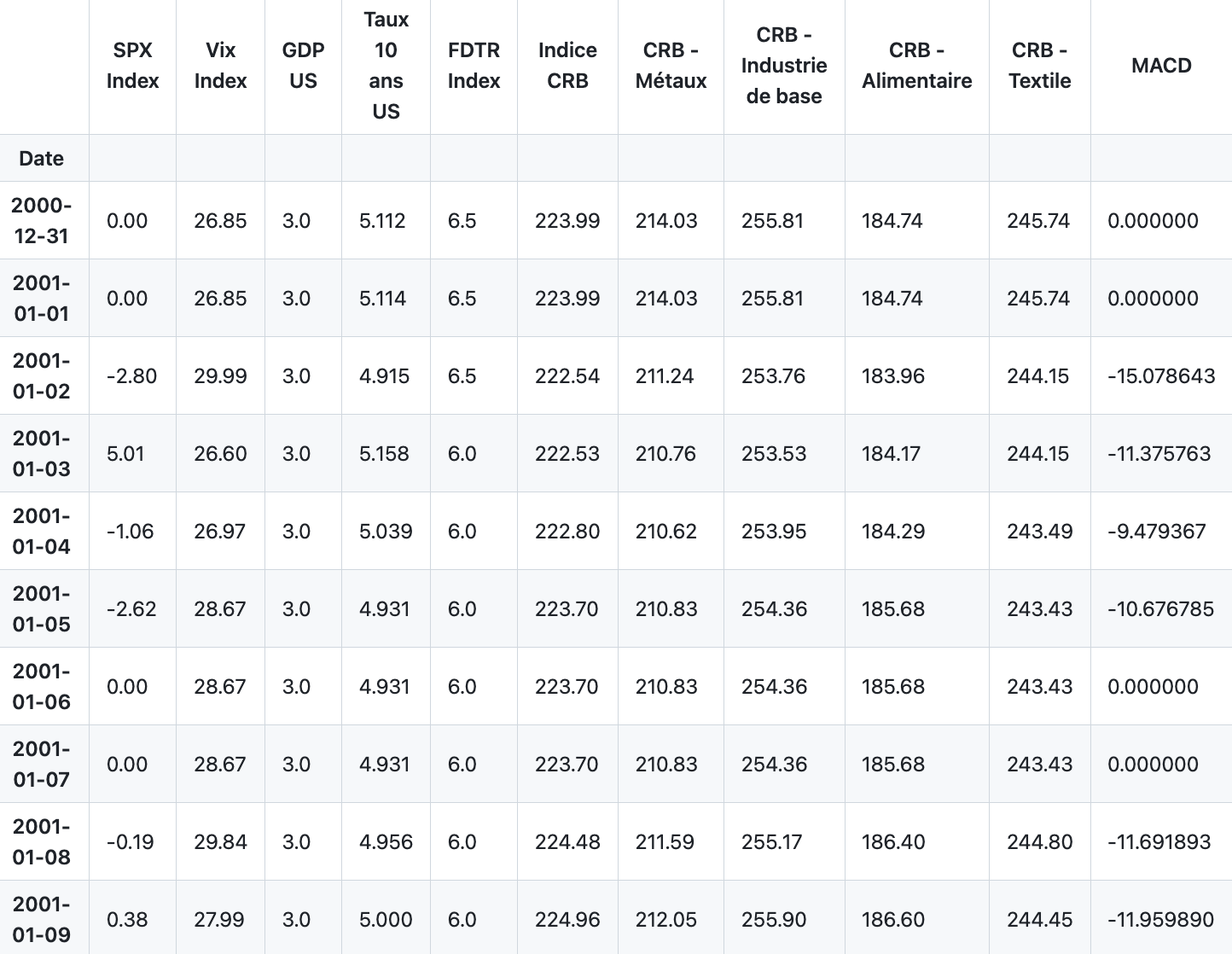
The code provided performs a series of data manipulation tasks using the pandas library in Python to handle and organize financial data from an Excel spreadsheet. First, it reads several sheets from an Excel file named dataset.xlsx. For each sheet, it sets the Date column as the index of the dataframe and makes sure this change is done in place without dropping the Date column. Then, it resamples the data for each dataframe at a daily frequency (D), using forward filling to handle missing values. Forward fill means it propagates the last valid observation forward until another valid observation is encountered. The specific data being manipulated consists of balance sheets (Bilan BC and Bilan FED), daily data (Données journalières), economical surprises (Surprise économique), gold prices (Or), inflation and unemployment data (Chômage & Inflation), oil prices (Pétrole), and production capacity data (Capacité de production). For the Données journalières dataframe, it additionally removes a column related to cattle (CRB — Bétail). Afterwards, it creates a new dataframe df_SPX derived from the SPX Index column of the daily data dataframe. The index for this new dataframe is copied from the daily datas index. Next, it joins all the previously resampled and manipulated dataframes with the daily data dataframe on their common index, which is the Date. Then, the code limits the scope of the data to be between December 31, 2000, and December 31, 2019. It then creates a new dataframe for SPX Index using the now joined daily data and resets its index. Finally, it displays the first 10 rows of the joined daily data dataframe using the head method.
sns.set(rc={'figure.figsize':(20, 9)})The provided line of code is a configuration instruction for the seaborn visualization library, which is commonly used in conjunction with matplotlib in Python for creating aesthetically pleasing and informative statistical graphs. The sns.set function is used to customize the visual properties of the plots generated by seaborn. Within the parentheses, rc refers to runtime configuration, which seaborn uses to control the style of the plots. By specifying the figure.figsize key, this line sets the size of the figures (plots) that seaborn will produce. The dimensions provided in the dictionary, (20, 9), represent the width and height of the figure in inches, respectively. After this code executes, any plots created with seaborn will have a default figure size of 20 inches in width and 9 inches in height until the size is modified again or the session is reset.
fig, ((ax1, ax2), (ax3, ax4)) = plt.subplots(2, 2, figsize=(14,8))
fig.suptitle('Macroeconomic indicators')
ax1.plot(df_daily_data['Vix Index'])
ax1.set_title("Vix Index")
ax2.plot(df_daily_data['GDP US'], 'tab:orange')
ax2.set_title("GDP US")
ax3.plot(df_daily_data['Taux 10 ans US'], 'tab:green')
ax3.set_title("10 years rate")
ax4.plot(df_daily_data['FDTR Index'], 'tab:red')
ax4.set_title("FDTR Index")

for ax in fig.get_axes():
    ax.label_outer()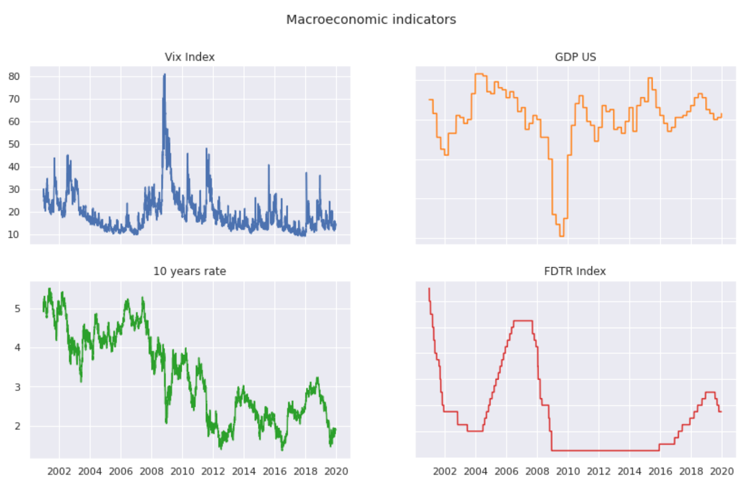
The provided code is for visualizing data using the matplotlib library in Python. It is creating a 2x2 grid of subplots with a specified size for a figure, meaning there will be four separate plots in one larger plotting area. The overall title for all subplots is set to Macroeconomic indicators. Each subplot is dedicated to plotting a different economic indicator taken from the df_daily_data dataframe. The upper left plot (ax1) shows the Vix Index, the upper right plot (ax2) displays the GDP of the US in orange, the lower left plot (ax3) presents the 10-year treasury rate of the US in green, and the lower right plot (ax4) visualizes the FDTR Index in red. Each subplot has its own title corresponding to the data it represents. Additionally, the code adjusts the labels of all the subplots to only display the outer ones to prevent overlapping and to keep the layout tidy.
plt.figure(figsize=(14,6))
plt.plot(df_daily_data["Indice CRB"], label="CRB Index")
plt.plot(df_daily_data["CRB - Métaux"], label="CRB Metals")
plt.plot(df_daily_data["CRB - Industrie de base"], label="Basic industries")
plt.plot(df_daily_data["CRB - Alimentaire"], label="Livestock")
#plt.ylabel('commo', fontsize=16)
plt.xlabel('Date')
plt.title('Commodity')
plt.legend()
The code snippet creates a line plot visualization using data from a dataframe called df_daily_data. First, it sets up the figure size to be 14 inches wide and 6 inches tall. Then, it plots four different time series from the dataframe: the CRB Index, CRB Metals, CRB Basic Industries, and CRB Livestock, each labeled accordingly. The y-axis label code is commented out, so it does not set a label for the y-axis. It sets the label for the x-axis to Date, and it specifies a title for the plot as Commodity. Finally, it adds a legend to the plot, which helps identify each line with its corresponding label. The designed plot helps in analyzing and comparing the trends over time for these different commodity indices.
Compute closing price
def compute_price(df):
  df['Closing Price'] = 1320.28*(1+df['SPX Index'].copy()/100).cumprod()
  return df
This code defines a function compute_price that takes a pandas DataFrame df as its argument. It calculates the cumulative product of the SPX Index column after increasing its values by 1 (to adjust for percentage change), effectively compounding the index values starting from 100%. This cumulative product is then multiplied by the number 1320.28, simulating the closing price of some financial instrument based on the performance of the SPX Index. The result of this calculation is assigned to a new column in the DataFrame called Closing Price. Finally, the function returns the modified DataFrame which now includes the Closing Price column with the computed values.
df_daily_data = compute_price(df_daily_data)The line of code provided appears to be a Python function call. The function compute_price() is being called with an argument df_daily_data. This is likely a pandas DataFrame that contains daily data, perhaps related to financial stock prices or some other type of daily metrics. The function compute_price() is expected to perform some operations on the DataFrame, such as computing new prices or updating existing prices based on certain criteria or calculations. The result of this computation is then assigned back to the variable df_daily_data, meaning that df_daily_data will be updated with the new computed prices. The specifics of these operations are not provided in the snippet given, but overall, the code updates df_daily_data with computed price information.