Every Machine Learning Algorithms For Beginners With Code

Best machine learning algorithms for begineers with coding samples in Python.

Jun 09, 2022

∙ Paid

There are many types of machine learning applications and research being pursued by academia and industry. It has a significant impact on every aspect of our lives. From machine learning and natural language processing enabled voice assistants that can make appointments, check our calendars, and play music, to programmatic advertisements that predict what we will need before we even consider it.

It can be challenging to stay on top of "what is important" in the scientific field of machine learning due to the sheer complexity of the field. But we also have to make sure that those who want to learn machine learning but are new to these concepts, can follow a learning path. Let's take a look at some of the most crucial basic algorithms that will hopefully make your machine learning journey a little easier.

person with assorted-color paint on face — Photo by h heyerlein on Unsplash

What Is Machine Learning?

As a child grows, so does machine learning. When a child grows, she gains more experience E in performing task T, resulting in higher performance measures (P).

A child might receive a "shape sorting block" toy. There are different shapes and shape holes in this toy. Task T in this case consists of finding a shaped hole that fits the shape. After observing the shape, the child attempts to fit it into the shaped hole. This toy has three shapes: a circle, a triangle, and a square. As a result of her first attempt at finding a shaped hole, her performance measure(P) is 1/3, which means she found one correct shape hole out of three.

After trying it again, the child notices that she has some experience in this task. As a result of the experience gained (E), the child attempts this task one more time and measures the performance (P) as 2/3. It took the baby 100 repetitions to figure out which shape fits into which hole.

She gained experience (E), and performed better (P), and we notice that as the number of attempts to play with this toy increased. A higher level of performance also leads to a higher level of accuracy.

Machine learning is similar to such execution. Machines take tasks (T), execute them, and measure their performance (P). With a large amount of data, a machine's experience (E) increases over time, causing its performance (P) to be higher. As a result, our machine learning model's accuracy increases after going through all the data, resulting in very accurate predictions.

Why do we need Machine Learning?

As an example, we have a collection of images of cats and dogs. Cats and dogs should be grouped together. In order to do that, we need to determine different characteristics of animals, such as:

How many eyes does each animal have?
What is the eye colour of each animal?
What is the height of each animal?
What is the weight of each animal?
What does each animal generally eat?

Based on the answers to these questions, we form a vector. Our next step is to apply a set of rules, such as:

If height > 1 Feet and weight > 15 lbs, then it could be a cat.

For each data point, we have to create such a set of rules. In addition, we build a decision tree of if, else, if, and else statements and check whether it falls into any of the categories.

In the event that the results of this experiment were not successful because many animals were misclassified, this would provide a great opportunity for machine learning. The purpose of machine learning is to process the data with different types of algorithms and tell us which factor is more important when determining whether it is a cat or a dog.

By simplifying the rules, we can give ourselves greater accuracy instead of applying multiple sets. Previous methods didn't generate accurate predictions.

Machine learning models that can help us, are:

Object Recognition
Summarization
Prediction
Classification
Clustering
Recommender Systems

What is a Machine Learning Model?

An answer/question system based on machine learning takes care of processing machine-learning-related tasks. A machine learning algorithm represents data as it solves problems. Below are a few methods that are useful in tackling business problems related to the industry.

For example, consider that we are implementing an ML algorithm to convey a specific demographic or area to Google Adwords' ML system. The goal of such a task is to gain valuable insights from data while improving business outcomes.

Machine Learning Algorithms:

Regression (Predictions)

Regression is used for the continuous prediction of values.

Regression algorithms:

Linear Regression
Polynomial Regression
Exponential Regression
Logistic Regression
Logarithmic Regression

Classification

We use classification algorithms for predicting a set of items.

Classification algorithm:

K-nearest Neighbors
Random Forest
Naive Bayes
Decision Trees
Support Vector Machines

Clustering

We use clustering algorithms for summarization.

Clustering algorithm:

K-Means
Mean Shift
Hierarchical

Association

We use association algorithms for associating co-occurring items or events.

Anomaly Detection

Detecting anomalous behaviour and unusual cases, for example, fraud, is one of the purposes of anomaly detection.

Sequence Pattern Mining

Sequential pattern mining can be used to predict the next data event between two data examples.

Recommendation Systems

We use recommenders algorithms to build recommendation systems.

What makes Python the preferred language to implement machine learning algorithms?

The Python programming language is a popular and general-purpose programming language. Python is capable of writing machine learning algorithms. Python has a diverse variety of modules and libraries already implemented to make our lives easier. That's why data scientists are so fond of it.

Numpy: It is a Python library that is used to deal with arrays of n dimensions. Using Numpy, we can perform computations efficiently and effectively.
The SciPy toolbox includes a collection of numerical algorithms and domain-specific tools, including signal processing, optimization, and statistics. Scripty is an open-source library for scientific and high-performance computations.
Matplotlib is a popular plotting package that allows 2D and 3D plotting.
Scikit-learn: It is a free programming language library for machine learning. The program has most of the algorithms for classification, regression, and clustering, and it is compatible with the Python numerical libraries Numpy and Scipy.

Machine Learning algorithms classify into two groups:

Supervised Learning Algorithms
Unsupervised Learning Algorithms

Supervised Learning Algorithms:

The goal is to predict class.

Machine learning (or deep learning for now) is a branch of machine learning that involves inferring a function from labelled training data.

Data for training constitutes a set of (input, target)* pairs. The input may be a vector of features, and the target indicates what we want the function to do. Classification and regression are roughly two categories of supervised learning, depending on the type of *target*.

Categorical targets are used for classification; simple examples include image classification, as well as more advanced topics like machine translation and image captions. Continuous targets are used for regression. Stock prediction, image masking, and other applications fall under this category.

Let's look at an example of supervised learning to better understand it. Children are given 100 stuffed animals of all kinds, including ten lions, ten monkeys, ten elephants, and so on. In the next step, we teach the kid how to recognize different types of animals by their characteristics (features). A lion, for example, would have orange color. It may be an elephant if it is a large animal with a trunk.

As an example of supervised learning, we teach the kid how to distinguish animals. He should now be able to classify animals into the appropriate groups when we give him different animals.

The following example shows that he correctly classified 8/10 of his classifications. As a result, we can say that the kid did an excellent job. Likewise, computers are subject to the same rules. A huge number of data points with their actual labelled values (Labeled data is classified data into different groups along with their features values) are provided to them. During its training period, it learns from its different characteristics. Our trained model can be used to make predictions after the training period has ended. Its supervised learning algorithm is based on data that has already been labelled, so we have already fed it with labelled data. Labelled data is used in this example to make predictions.

Examples of supervised learning algorithms:

Linear Regression
Logistic Regression
K-Nearest Neighbors
Decision Tree
Random Forest

Unsupervised Learning:

As opposed to supervised learning. A function that describes hidden structures in data is inferred from unlabeled data by unsupervised learning.

Dimension reduction methods, such as PCA and t-SNE, are the simplest type of unsupervised learning, with PCA being used primarily in data preprocessing, and t-SNE used for visualization.

Those who would like to explore more advanced data patterns would use clustering, such as K-means clustering, Gaussian mixture models, hidden Markov models, and so on.

Unsupervised learning continues to gain popularity because it frees us from manually labelling data, much like the renaissance of deep learning. We consider two types of unsupervised learning in the light of deep learning: representation learning and generative models.

With representation learning, small, high-level features can be extracted that can be used for downstream tasks, while with generative models, hidden parameters can be used to reproduce the input data.

Unsupervised learning is exactly what it sounds like. The data are not labelled in this type of algorithm. Therefore, the machine has to process the input data and attempt to draw conclusions about the output. Did you remember that kid with the shape toy? To find the perfect shape hole for different shapes, he would learn from its mistakes.

Unfortunately, we do not give the child food by teaching methods to fit the shapes (known as labelled data for machine learning purposes). The child, however, tries to draw conclusions about the toy's characteristics. This is because he has no labelled data to draw conclusions from.

Examples of unsupervised learning algorithms:

Dimension Reduction
Density Estimation
Market Basket Analysis
Generative adversarial networks
Clustering

Linear Regression

An approach to modelling the relationship between features on the input side and features on the output side is linear regression. Typically, independent variables are referred to as input features, and dependent variables are referred to as output features. Based on the input features, we need to multiply it with the optimal coefficients to predict the value of the output.

Linear regression is used to predict sales of products, predict economic growth, and predict petroleum prices.

There are two types of linear regression:

Simple Linear Regression
Multivariable linear regression

Simple Linear Regression

By using only one input feature, we can predict the outcome/dependent variable. The simple linear regression equation is:

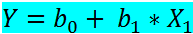
Here:

b0 = constant or y — intercept of line

b1 = coefficient of input feature

x1 = input feature on which output is based

y = output

In the following paragraphs, we will use the sklearn library to implement simple linear regression in Python.

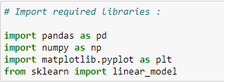
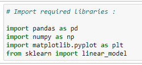
Step 1: Import Required Libraries:

We need to import libraries because we will use them for calculations.

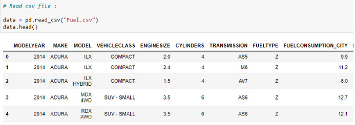
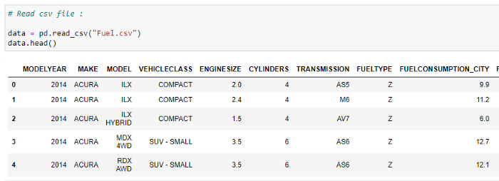
Read The CSV File:

Our dataset's first five rows are checked. We are examining a vehicle model dataset in this case - please visit Softlayer IBM to view the dataset.

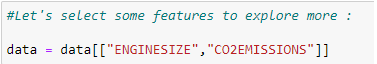
Choose the features we want to consider in predicting values:

The objective here is to predict the value of "co2 emissions" based on the value of "engine size" in our dataset.

Plot The Data:

Our data can be visualized on a scatter plot.

Dividing Data Into Training And Testing Data:

Using the training and testing datasets, we can determine the accuracy of a model. Training data will be used to train our model, and then testing data will be used to test the accuracy of our model.

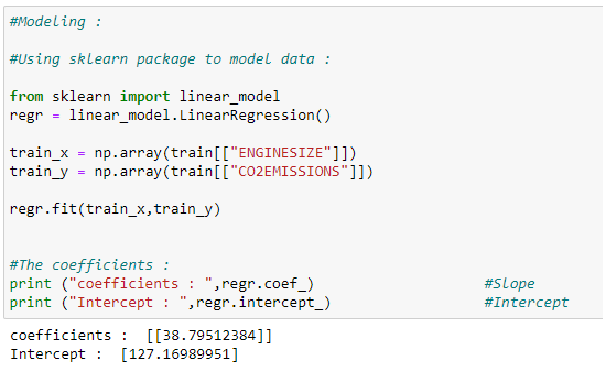
Training our Model:

In the following, we will learn how to train our model and find the coefficients of our best-fit regression line.

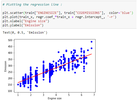
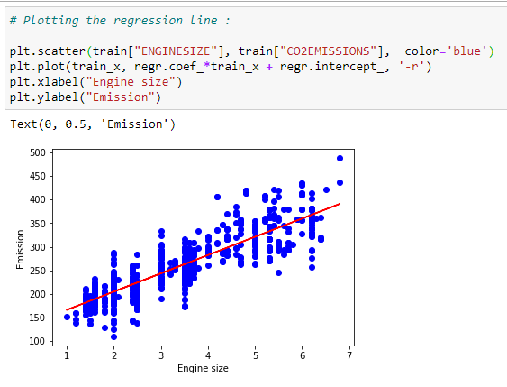
Plot the best fit line:

For our dataset, we can plot the best fit line based on the coefficients.

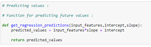
Prediction function:

We can plot the best fit line for our dataset using the coefficients.

Data plot for linear regression based on its coefficients | Source: Image created by the author.

Prediction function:

Our testing dataset will be modeled with a prediction function.

Predicting co2 emissions:

A regression line can be used to predict the values of carbon dioxide emissions.

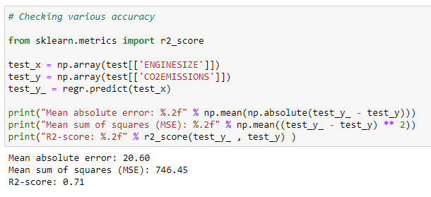
Checking accuracy for test data :

Comparison of actual and predicted values in our dataset can be used to test the accuracy of a model.

Putting it all together:

# Import required libraries:
import pandas as pd
import numpy as np
import matplotlib.pyplot as plt
from sklearn import linear_model# Read the CSV file :
data = pd.read_csv(“Fuel.csv”)
data.head()# Let’s select some features to explore more :
data = data[[“ENGINESIZE”,”CO2EMISSIONS”]]# ENGINESIZE vs CO2EMISSIONS:
plt.scatter(data[“ENGINESIZE”] , data[“CO2EMISSIONS”] , color=”blue”)
plt.xlabel(“ENGINESIZE”)
plt.ylabel(“CO2EMISSIONS”)
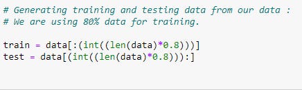
plt.show()# Generating training and testing data from our data:
# We are using 80% data for training.
train = data[:(int((len(data)*0.8)))]
test = data[(int((len(data)*0.8))):]# Modeling:
# Using sklearn package to model data :
regr = linear_model.LinearRegression()
train_x = np.array(train[[“ENGINESIZE”]])
train_y = np.array(train[[“CO2EMISSIONS”]])
regr.fit(train_x,train_y)# The coefficients:
print (“coefficients : “,regr.coef_) #Slope
print (“Intercept : “,regr.intercept_) #Intercept# Plotting the regression line:
plt.scatter(train[“ENGINESIZE”], train[“CO2EMISSIONS”], color=’blue’)
plt.plot(train_x, regr.coef_*train_x + regr.intercept_, ‘-r’)
plt.xlabel(“Engine size”)
plt.ylabel(“Emission”)# Predicting values:
# Function for predicting future values :
def get_regression_predictions(input_features,intercept,slope):
 predicted_values = input_features*slope + intercept
 return predicted_values# Predicting emission for future car:
my_engine_size = 3.5
estimatd_emission = get_regression_predictions(my_engine_size,regr.intercept_[0],regr.coef_[0][0])
print (“Estimated Emission :”,estimatd_emission)# Checking various accuracy:
from sklearn.metrics import r2_score
test_x = np.array(test[[‘ENGINESIZE’]])
test_y = np.array(test[[‘CO2EMISSIONS’]])
test_y_ = regr.predict(test_x)print(“Mean absolute error: %.2f” % np.mean(np.absolute(test_y_ — test_y)))
print(“Mean sum of squares (MSE): %.2f” % np.mean((test_y_ — test_y) ** 2))
print(“R2-score: %.2f” % r2_score(test_y_ , test_y) )

Multivariable Linear Regression:

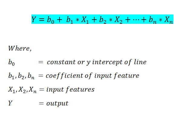
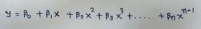
We were only able to use one input feature in simple linear regression for predicting the output value. Multivariate Linear Regression, however, allows us to predict the outcome based on more than one input feature. Below is the multivariate linear regression formula.

Step by step implementation in Python:

Import the required libraries:

Read the CSV file :

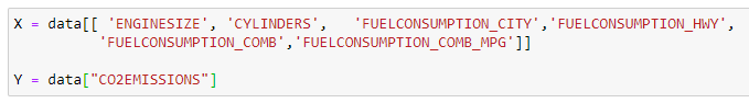
Define X and Y:

X keeps track of the input features, and Y keeps track of the output value.

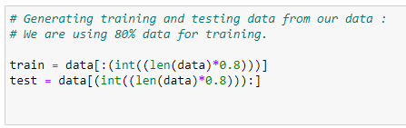
Divide data into a testing and training dataset:

80% of the data will be used for training and 20% for testing.

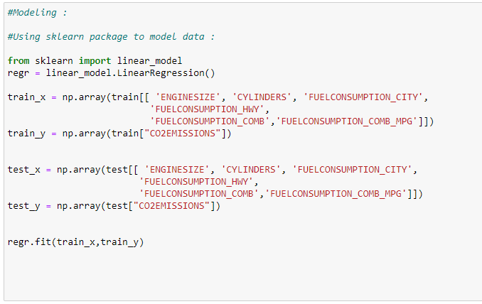
Train our model :

In this case, we will train our model with 80% of the data.

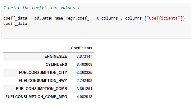
Find the coefficients of input features :

The next step is to identify which feature has a greater impact on the output variable. This can be done by looking at the coefficient values. This means it has an inverse effect on the output, as indicated by the negative coefficient. The output value decreases if the value of that feature increases.

Predict the values:

Accuracy of the model:

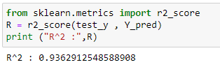
Observe that for both simple and multivariable linear regression, we used the same dataset. As can be seen, multivariable linear regression is much more accurate than simple linear regression.

Putting it all together:

# Import the required libraries:
import pandas as pd
import numpy as np
import matplotlib.pyplot as plt
from sklearn import linear_model# Read the CSV file:
data = pd.read_csv(“Fuel.csv”)
data.head()# Consider features we want to work on:
X = data[[ ‘ENGINESIZE’, ‘CYLINDERS’, ‘FUELCONSUMPTION_CITY’,’FUELCONSUMPTION_HWY’, 
 ‘FUELCONSUMPTION_COMB’,’FUELCONSUMPTION_COMB_MPG’]]Y = data[“CO2EMISSIONS”]# Generating training and testing data from our data:
# We are using 80% data for training.
train = data[:(int((len(data)*0.8)))]
test = data[(int((len(data)*0.8))):]#Modeling:
#Using sklearn package to model data :
regr = linear_model.LinearRegression()train_x = np.array(train[[ ‘ENGINESIZE’, ‘CYLINDERS’, ‘FUELCONSUMPTION_CITY’,
 ‘FUELCONSUMPTION_HWY’, ‘FUELCONSUMPTION_COMB’,’FUELCONSUMPTION_COMB_MPG’]])
train_y = np.array(train[“CO2EMISSIONS”])regr.fit(train_x,train_y)test_x = np.array(test[[ ‘ENGINESIZE’, ‘CYLINDERS’, ‘FUELCONSUMPTION_CITY’,
 ‘FUELCONSUMPTION_HWY’, ‘FUELCONSUMPTION_COMB’,’FUELCONSUMPTION_COMB_MPG’]])
test_y = np.array(test[“CO2EMISSIONS”])# print the coefficient values:
coeff_data = pd.DataFrame(regr.coef_ , X.columns , columns=[“Coefficients”])
coeff_data#Now let’s do prediction of data:
Y_pred = regr.predict(test_x)# Check accuracy:
from sklearn.metrics import r2_score
R = r2_score(test_y , Y_pred)
print (“R² :”,R)

Polynomial Regression:

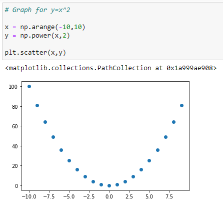
In some cases, we have data that does not follow a linear trend. Polynomial trends are sometimes seen. For this reason, we will apply polynomial regression. It is essential to know how polynomial graphs look before diving into their implementation.

Polynomial Functions and Their Graphs:

Graph for Y=X:

Graph for Y = X²:

Graph for Y = X³:

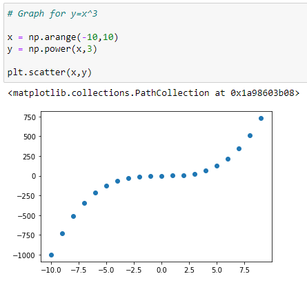
Graph with more than one polynomials: Y = X³+X²+X:

In the graph above, we can see that the red dots show the graph for Y=X³+X²+X and the blue dots shows the graph for Y = X³. Here we can see that the most prominent power influences the shape of our graph.

Below is the formula for polynomial regression:

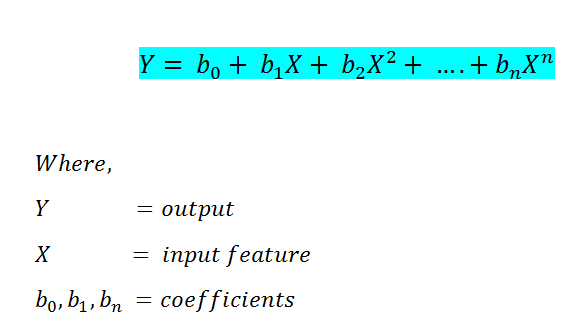
The formula for a polynomial regression | Source: Image created by the author.

Now, when we implemented our regression models in the past, we used the Scikit-Learn library. The Normal Equation will be used to implement this. You will notice that we can also implement polynomial regression with scikit-learn, but another method will help us better understand how it works.

The equation goes as follows:

In the equation above:

θ: hypothesis parameters that define it the best.

X: input feature value of each instance.

Y: Output value of each instance.

Hypothesis Function for Polynomial Regression

Source: Image created by the author.

The main matrix in the standard equation:

Step by step implementation in Python:

Import the required libraries:

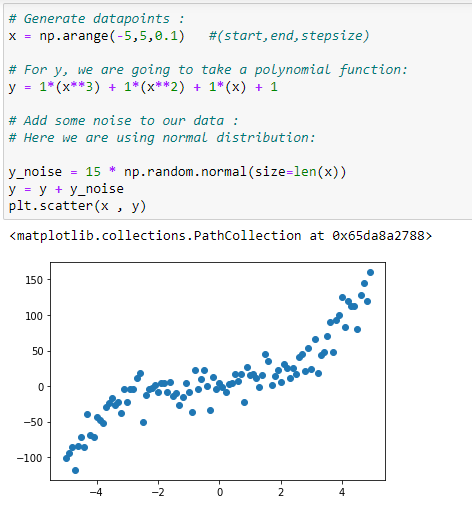
Generate the data points:

Our polynomial regression will be implemented based on a dataset.

Initialize x,x²,x³ vectors:

We are taking the maximum power of x as 3. So our X matrix will have X, X², X³.

Column-1 of X matrix:

In the main matrix X, the first column will always be 1 since it holds the beta_0 coefficient.

Form the complete x matrix:

At the start of this implementation, we have the matrix X. We will create it by appending vectors to it.

Transpose of the matrix:

Our next step will be to calculate theta's value step-by-step. Let's start by determining the matrix transpose.

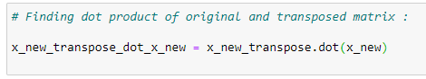
Matrix multiplication:

The transpose must be multiplied by the original matrix once it is found. The equation has to be implemented with a normal equation, so we have to follow the rules of that equation.

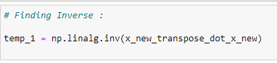
The inverse of a matrix:

Storing the inverse of the matrix in temp1 after finding the inverse of the matrix.

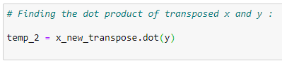
Matrix multiplication:

A variable temp2 is created by multiplying transposed X and Y vectors.

Coefficient values:

By multiplying temp1 and temp2, we can find the coefficient values. This is the formula for normal equations.

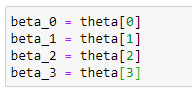
Store the coefficients in variables:

Storing those coefficient values in different variables.

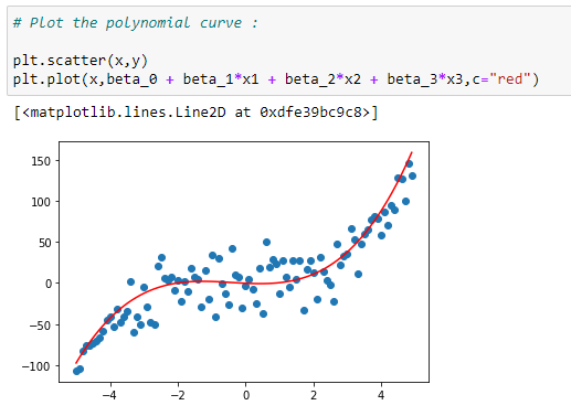
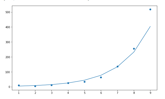
Plot the data with a curve:

Plotting the data with the regression curve.

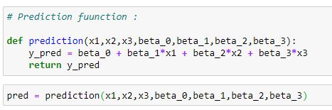
Prediction function:

The regression curve will now be used to predict the output.

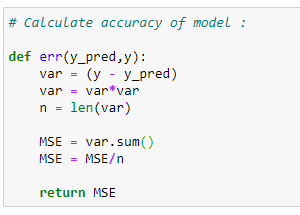
Error function:

Use the mean squared error function to calculate the error.

Calculate the error:

Putting it all together:

# Import required libraries:
import numpy as np
import matplotlib.pyplot as plt# Generate datapoints:
x = np.arange(-5,5,0.1)
y_noise = 20 * np.random.normal(size = len(x))
y = 1*(x**3) + 1*(x**2) + 1*x + 3+y_noise
plt.scatter(x,y)# Make polynomial data:
x1 = x
x2 = np.power(x1,2)
x3 = np.power(x1,3)# Reshaping data:
x1_new = np.reshape(x1,(n,1))
x2_new = np.reshape(x2,(n,1))
x3_new = np.reshape(x3,(n,1))# First column of matrix X:
x_bias = np.ones((n,1))# Form the complete x matrix:
x_new = np.append(x_bias,x1_new,axis=1)
x_new = np.append(x_new,x2_new,axis=1)
x_new = np.append(x_new,x3_new,axis=1)# Finding transpose:
x_new_transpose = np.transpose(x_new)# Finding dot product of original and transposed matrix :
x_new_transpose_dot_x_new = x_new_transpose.dot(x_new)# Finding Inverse:
temp_1 = np.linalg.inv(x_new_transpose_dot_x_new)# Finding the dot product of transposed x and y :
temp_2 = x_new_transpose.dot(y)# Finding coefficients:
theta = temp_1.dot(temp_2)
theta# Store coefficient values in different variables:
beta_0 = theta[0]
beta_1 = theta[1]
beta_2 = theta[2]
beta_3 = theta[3]# Plot the polynomial curve:
plt.scatter(x,y)
plt.plot(x,beta_0 + beta_1*x1 + beta_2*x2 + beta_3*x3,c=”red”)# Prediction function:
def prediction(x1,x2,x3,beta_0,beta_1,beta_2,beta_3):
 y_pred = beta_0 + beta_1*x1 + beta_2*x2 + beta_3*x3
 return y_pred
 
# Making predictions:
pred = prediction(x1,x2,x3,beta_0,beta_1,beta_2,beta_3)
 
# Calculate accuracy of model:
def err(y_pred,y):
 var = (y — y_pred)
 var = var*var
 n = len(var)
 MSE = var.sum()
 MSE = MSE/n
 
 return MSE# Calculating the error:
error = err(pred,y)
error