

Every Supervised Learning Algorithm
As one of the most important types of modern algorithms, supervised machine learning algorithms will be discussed in this article.

Machine learning algorithms that use labeled data to train models are known as supervised algorithms. All traditional supervised machine learning algorithms will be discussed in this article, with the exception of neural networks.
We are now going to discuss supervised machine learning algorithms in two parts. Introducing supervised machine learning fundamentals is the first step. Following that, we will discuss two types of supervised machine models: classifiers and regressors. A real-world problem will be presented as a challenge to demonstrate the capabilities of classifiers. To solve this problem, six different classification algorithms will be presented. Our next focus will be on regression algorithms, first presenting a similar problem for regressors to solve. The next step in solving the problem is to present three regression algorithms. Finally, we will summarize this article’s concepts by comparing the results.
As a result of this article, you should have an understanding of the different kinds of supervised machine learning methods, as well as what is the best supervised machine learning technique for certain types of problems.
In this article, we discuss the following topics:
A comprehensive understanding of supervised machine learning
Classification algorithms: an understanding
A method for evaluating the performance of classifiers
Regression algorithms: an understanding
Regression algorithms are evaluated by using the following methods
The basics of supervised machine learning should be explained first.
Learning about supervised machine learning
With machine learning, we can create autonomous systems that make decisions without human supervision by using data-driven approaches. These autonomous systems are created through machine learning, which employs algorithms and methodologies to discover and formulate repeatable patterns in data.
In machine learning, supervised machine learning is a popular and powerful approach. Assisted machine learning involves giving an algorithm a set of inputs, called features, and their corresponding outputs, called target variables. In supervised machine learning, a mathematical formula is used to capture the complex relationship between features and target variables given a dataset. The trained model serves as the basis for making predictions.
In order to make predictions, the trained model is used to generate an unfamiliar target variable.
Similar to the way the human brain learns from experience, supervised learning is able to learn from existing data. In supervised learning, this ability to learn relies on a human brain characteristic and opens the door to machines that can make decisions and make intelligent decisions.
In the example below, let’s use supervised machine learning to train a model that can recognize legitimate emails (called legit) from unwanted ones (called spam). We need examples from the past before we can get started so that the machine can learn what type of content should be classified as spam. One of the supervised machine learning algorithms is used to accomplish this task for content-based learning for text data. In this article, we will discuss decision trees and naive Bayes classifiers as examples of supervised machine learning algorithms that can be used to train this example’s model.
The formulation of supervised machine learning algorithms
The following terms should be defined before we go deeper into supervised machine learning algorithms: Terminology with their explanations.
Target variable
Models predict variables based on their target variables. In supervised machine learning, only one target variable can be chosen.
Label
Labels refer to category variables that we want to predict.
Features
Features are input variables used to predict labels.
Feature engineering
Feature engineering involves transforming features so they can be used in supervised machine learning algorithms.
Feature vector
Feature vectors are data structures that combine all the features before being fed into a supervised machine learning algorithm.
Historical data
Historical data can be used to formulate the relationship between a target variable and a feature. The historical data is accompanied by examples.
Training/testing data
There are two parts to historical data with examples: a training dataset and a testing dataset.
Model
A formula for the patterns that best capture the relationship between the features and the target variable.
Training
Training data is used to create a model.
Testing
Test data are used to evaluate the model’s quality.
Prediction
Predicting the target variable with a model.
By estimating the target variable from the features, a trained supervised machine learning model can make predictions.
This article will cover machine learning techniques using the following notation:
y:
Actual label
ý:
Predicted label
d:
Total number of examples
b:
Number of training examples
c:
Number of testing examples
We will now look at some practical examples of these terminologies.
Feature vectors are data structures that store all the features, as we discussed earlier.
In this case, X_train represents the training feature vector if n is the number of features and b is the number of training examples. The feature vector consists of rows for each example.
X_train represents the feature vector for the training dataset. X_train will contain b rows if there are b examples in the training dataset. In a training dataset with n variables, there will be n columns. Accordingly, the training dataset will have a dimension of n x b, as shown below:

Assume there are examples of b training and c testing. (X, Y) is the representation of a particular training example.
In the training set, we use superscripts to identify which training example is which.
We can therefore represent our labeled dataset as D = [X(1),y(1)), (X(2),y(2)), — (X(d),y(d)].
There are two parts to that — Dtrain and Dtest.
In other words, we can represent our training set as Dtrain = [X(1),y(1)), (X(2),y(2)), -, (X(b),y(b)].
During training, the goal is that the predicted value of the target value for every example in the training set should be as close as possible to the actual value. In other words,

The testing set can be represented as Dtest = [X(1),y(1)), (X(2),y(2)), — , (X(c),y(c)].
The values of the target variable are represented by a vector, Y:
Y ={ y(1), y(2), ….., y(m)}Identifying enabling conditions
With supervised machine learning, a model is trained using examples provided by an algorithm. There are certain enabling conditions that must be met in order for supervised machine learning algorithms to work. The following conditions enable this:
Models can only be trained with enough examples in supervised machine learning algorithms.
Historical data must contain patterns in order to train a model. We should combine patterns, trends, and events to determine the likelihood of occurrence of our event. Models cannot be trained without these, and we are left with random data.
The assumptions that apply to examples when we train a supervised machine learning model will also be valid in the future. Here is an example we can look at. The understanding is that when we train a machine learning model to predict whether a student will be granted a visa, the laws and policies will not change. The model may need to be retrained if new policies or laws are implemented after it has been trained.
Identifying classifiers and regressors
Machine learning models can use continuous or category variables as target variables. We have various types of supervised machine learning models depending on the type of target variable. A supervised machine learning model can be classified into two types:
A classifier is a machine learning model that uses a category variable as a target variable. There are several types of business questions that can be answered using classifiers:
Do you think this is a malignant tumor?
Is tomorrow likely to be a rainy day based on the weather conditions today?
Is it appropriate to approve a mortgage application based on the profile of the applicant?
In the case of continuous variables, a regressor is trained. Business questions can be answered with regressions in the following ways:
What is the probability of rain tomorrow based on the current weather conditions?
With given characteristics, what is the expected price of a particular home?
Here are some details on classifiers and regressors.
Algorithm understanding
A supervised machine learning model is classified as a classifier if the target variable is a category variable:
Labels are used to identify the target variable.
Data that has been labeled historically is called labeled data.
Labels must be predicted for unlabeled data, which is production data.
The real power of classification algorithms lies in their ability to accurately label unlabeled data. In order to answer a particular business question, classification algorithms predict labels for unlabeled data.
As a challenge for classifiers, let’s present a business problem before we introduce the details of classification algorithms. Then, we will compare the methodology, approach, and performance of six algorithms by answering the same challenge.
A challenge for classifiers
To test six different classification algorithms, we will first present a common problem. Classifier challenges are referred to in this article as this common problem. In solving the same problem with all six classifiers, we will be able to do two things:
Assembling a feature vector involves processing and organizing all the input variables. We can avoid repeating data preparation for all six algorithms if we use the same feature vector.
By using the same feature vector for input, we can compare the performance of different algorithms.
In the classifier challenge, you must predict whether someone will make a purchase. Understanding customers’ behavior is one of the things that can help maximize sales in the retail industry. In order to do this, historical data can be analyzed for patterns. First, let’s define the issue.
Problem statement
Does the historical data allow us to train a binary classifier to predict whether a particular user will eventually purchase a product?
The first step in solving this problem is to explore the historical labeled data set:
x € ℜb, y € {0,1}A positive class is one when y = 1, while a negative class is one when y = 0.
Defining the positive class as the event of interest is a good practice even though the level of the positive and negative classes can be arbitrarily defined. In order to flag a fraudulent transaction for a bank, the positive class (y = 1) should represent the fraudulent transaction, not the negative class (y = 0).
Here are a few things to consider:
This is the actual label, denoted by y
Label predicted by y`
It is important to note that in our classifier challenge, the actual value of the label is represented by y. When someone purchases an item, we say y = 1. As a result of this prediction, we have y`. X is a four-dimensional feature vector in the input. Given a particular input, we want to figure out what the likelihood is that a user will make a purchase.
Given a particular value of feature vector x, we want to calculate the probability of y = 1. We can represent this mathematically as follows:

Let’s examine how to process and assemble different input variables in the feature vector, x. In the following section, we discuss more in detail the methodology for assembling different parts of x.
The use of a data processing pipeline to engineer features
As part of the machine learning life cycle, feature engineering is a crucial step in preparing data for machine learning algorithms. Different phases or stages are involved in feature engineering. A data pipeline is a set of multistage processing codes that process data. Whenever possible, create a data pipeline with standard processing steps to make it reusable and decrease training time. The quality of the code is also improved by using more well-tested software modules.
For the classifiers challenge, let’s design a reusable pipeline. All the classifiers will use the same data that we prepare once.
Data import
.csv files are used to store historical data on this problem. The data will be imported into a pandas data frame using the pd.read_csv function:

Feature selection
Feature selection involves selecting features that are relevant to the problem we are trying to solve. In feature engineering, it plays an essential role.
The User ID column, which is used to identify people, is dropped after the file is imported:

Here is a preview of the dataset:

Below is a screenshot of the dataset:

Let’s examine how the input dataset can be further processed.
One-hot encoding
It is common for machine learning algorithms to require continuous variables for all the features. It means we need to find a way to transform some of the features into continuous variables if they are category variables. In order to achieve this transformation, one-hot encoding is the most effective method. As far as this particular problem is concerned, we only have a category variable called Gender. We can convert that into a continuous variable using one-hot encoding as follows:

Here is the dataset after it has been converted:

A one-hot encoding has converted Gender into two separate columns, Male and Female, in order to convert it from a category variable to a continuous variable.
Defining features and labels
The features and labels need to be specified. Labels will be represented by y and feature sets by X throughout this article:
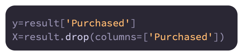
All the input variables that are used to train the model can be found in X, which represents a feature vector.
Separating the dataset into training and testing parts
With sklearn.model_selection import train_test_split, we will divide the test dataset into 25% and 75% of the training dataset:

Four data structures have been created as a result:
The training data is stored in a data structure called X_train
A data structure containing the features of the training test, X_test
In the training dataset, y_train contains the label values
In the testing dataset, y_test contains the values of the label
Feature scaling
Scaling variables from 0 to 1 is a good practice for many machine learning algorithms. Feature normalization is the process of normalizing features. Using the scaling transformation, we can accomplish this:
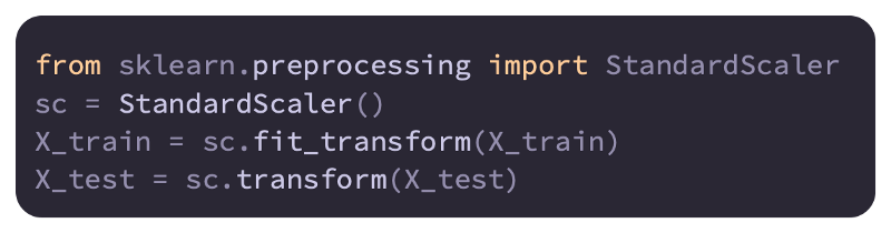
We will present different classifiers in the subsequent sections after scaling the data.
Classifier evaluation
We must evaluate the performance of the model once it has been trained. In order to accomplish this, we will follow these steps:
A training partition and a testing partition will be created from the labeling dataset. In order to evaluate the trained model, we will use the testing partition.
To generate labels for each row, we will use the features of our testing partition. Predicted labels are shown here.
The model will be evaluated by comparing predicted labels with actual labels.
When we evaluate a model, at least some misclassifications are likely to occur unless the problem is quite trivial. Depending on which performance metrics we use, we interpret these misclassifications to determine the quality of the model.
In order to evaluate the models, we need both the actual labels as well as the predicted labels. Choosing the best metric will depend on the business problem and the training dataset, as well as the requirements of the model.
A matrix of confusion
Classifier evaluation results are summarized in a confusion matrix. Binary classifiers have the following confusion matrix:

Classifiers that have two levels of labels are referred to as binary classifiers. A binary classifier was used during the First World War as the first critical use case of supervised machine learning.
Four categories can be distinguished:
A true positive (TP) is a classification that was correctly classified as positive
TNs (True Negatives): Correctly classified negative classifications
A false positive (FP) is a positive classification that is actually a negative classification
An example of a false negative (FN) would be when a positive classification was actually classified as a negative
Using these four categories, we can create a variety of performance metrics.
Metrics of performance
Model performance is quantified by performance metrics. Let’s define four metrics based on this:
Accuracy

Recall

Precision

F1 score
Prediction accuracy is the percentage of correct classifications among all predictions. TP and TN are not differentiated when calculating accuracy. It is straightforward to evaluate a model based on accuracy, but it is not always effective.
Let’s consider situations where a model’s performance needs to be quantified beyond accuracy. The following examples illustrate how we might use a model to predict a rare event:
In a bank transactional database, a model to predict fraudulent transactions is developed
An aircraft engine failure prediction model
We are trying to predict a rare event in both of these examples. Recall and precision are two additional measures that become more important than accuracy in these situations. Here are a few examples:
Recall: The hit rate is calculated here. The first example shows the percentage of fraudulent documents correctly flagged by the model. The model identified 78 fraudulent transactions out of one million transactions in our testing dataset, out of which 100 were known to be fraudulent. 78/100 would be the recall value in this case.
Precision measures how many of the transactions flagged by the model are actually bad. It would be more helpful to determine the precision of the bad bins flagged by the model rather than only concentrating on the bad transactions that the model failed to flag.
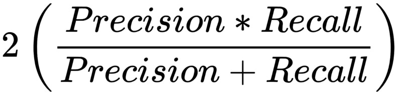
F1 combines recall and precision. An F1 score will be perfect if a model has perfect recall and precision scores. Having a high F1 score means that the model has been trained well and has a high recall rate and precision rate.
Overfitting: An understanding
In a production environment, we say the model is overfitted if the performance is poor in a development environment. As a result, the trained model too closely resembles the training dataset. This indicates the model’s rules have too many details. A trade-off between model variance and bias is the best way to summarize the idea. As we go through these concepts one by one, let’s take a closer look at each.
Bias
There are certain assumptions that go into training any machine learning model. A few real-world phenomena are approximated with these assumptions. The assumptions simplify the actual relationships between features and their characteristics, making it easier to train a model. The more assumptions you make, the more biased you are. A model’s bias increases when it is trained using simplistic assumptions, whereas a model’s bias decreases when realistic assumptions are used.
It ignores features’ non-linearity and approximates them as linear variables in linear regression. Thus, linear regression models tend to exhibit high bias by nature.
The variance
Using a different dataset to train the model, a model’s variance is quantified. Our model quantifies whether our mathematical formulation generalizes the underlying patterns well.
An overfitted rule based on a specific scenario or situation = high variance, and an overfitted rule based on a generalized scenario or situation = low variance.
A low bias and low variance model is what we aim for when we train machine learning models. Often, data scientists stay up at night worrying about achieving this goal.
The bias-variance trade-off
In training a machine learning model, it can be challenging to decide what level of generalization to use for its rules. In the bias-variance trade-off, the struggle to find the right generalization level is captured.
The more simplistic the assumptions, the more generalized the results, and the lower the variance, the higher the variance.
Data characteristics, algorithm choice, and various hyperparameters determine how bias and variance are balanced. Depending on the requirements of the specific problem you are trying to solve, you need to achieve the right compromise between bias and variance.
Defining the phases of a classifier
A classifier’s development begins with labeled data, followed by training, evaluation, and deployment. The following diagram shows the three phases of implementing a classifier in accordance with CRISP-DM (Cross-Industry Standard Process for Data Mining).

A classifier is tested and trained using labeled data in the first two phases. Two partitions are created from the labeled data: one is the training partition and the other is the testing partition. To ensure both training and testing partitions contain consistent patterns, input labeled data is divided randomly into training and testing partitions. A model is trained using training data, as shown in the preceding diagram. A trained model is evaluated using testing data after it has completed the training phase. Model performance is quantified using different performance matrices. Model deployment occurs once the model is evaluated, when the trained model is deployed and used to label unlabeled data to solve real-world problems.
Here are some algorithms for classifying data.
The following algorithms will be discussed in the following sections:
The decision tree algorithm
The XGBoost algorithm
The random forest algorithm
The logistic regression algorithm
The Support Vector Machine (SVM) algorithm
The naive Bayes algorithm
The decision tree algorithm should be the first thing we look at.
Classification algorithm based on decision trees
In a decision tree, a set of rules is generated through recursive partitioning (divide and conquer), which can be used to predict a label. Multiple branches branch off from a root node. A branch to the next level represents the result of a test on a specific attribute. Ultimately, the decision tree ends with leaf nodes containing the decisions. When partitioning does not improve the outcome, the process ends.
Using decision trees to classify data
Human-interpretable rules are generated at runtime to predict the label using decision trees. Algorithms are recursive in nature. In order to create this hierarchy of rules, follow these steps:
Out of all the features in the training dataset, the algorithm identifies the feature that distinguishes the data points best according to the labels. Information gain and Gini impurity are used as metrics for the calculation.
A bifurcation algorithm divides the training dataset into two branches by using the most identified important feature:
Those data points that meet the criteria
Those data points that do not meet the criteria
The resultant branch is made final if it mostly contains labels of one class.
The algorithm will go back to step 1 if the provided stopping conditions are not met. Otherwise, the decision tree nodes at the lowest level are labelled as leaf nodes and the model is marked as trained. Alternatively, the algorithm can stop as soon as each leaf node reaches a certain homogeneity level, which is defined as the number of iterations.
The following diagram illustrates the decision tree algorithm:

A bunch of circles and crosses make up the root of the diagram above. In the algorithm, circles and crosses are separated based on a criterion. The decision tree creates partitions of data at each level, which are expected to become more homogeneous as they progress. There are only two types of leaf nodes in a perfect classifier: circles and crosses. The inherent randomness of the training dataset makes it difficult to train perfect classifiers.
For the classifiers challenge, we used the decision tree algorithm
Let’s use the decision tree classification algorithm to predict whether a customer will buy a product based on the problem we previously defined:
Let’s begin by implementing the decision tree classification algorithm and then training a model using the training set of data we prepared.

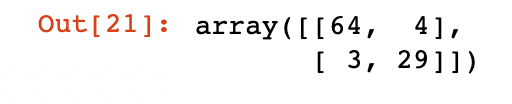
With our trained model, we can now predict the labels for our labeled testing data. To summarize our trained model’s performance, let’s generate a confusion matrix:

As a result, we get the following:

With the decision tree classification algorithm, we can now calculate the accuracy, recall, and precision values for the created classifier:

The following output will be produced by running the preceding code:

Comparisons between different training model techniques can be made using performance measures.
Decision tree classifiers: strengths and weaknesses
Let’s examine the advantages and disadvantages of using the decision tree classification algorithm in this section.
Aspects of strength
A decision tree classifier has the following strengths:
By using a decision tree algorithm, models can be created that can be interpreted by humans. These types of models are known as whitebox models. When transparency is needed to trace the details and reasons behind decisions made by a model, whitebox models are required. For applications that protect vulnerable communities and prevent bias, transparency is essential. The government and insurance industries, for instance, typically require whitebox models.
A decision tree classifier takes information from a discrete problem space and extracts it as knowledge. Using a decision tree to train the model makes sense since most of the features are category variables.
Weaknesses
A decision tree classifier has the following weaknesses:
An overfitted model is created when the decision tree classifier generates a tree with too many details. In order to prevent overfitting, we need to prune decision trees whenever necessary when we use a decision tree algorithm.
In decision tree classifiers, nonlinear relationships are not captured in the rules they generate.
Use cases
The purpose of this section is to discuss the use cases of the decision tree algorithm.
Classifying records
Using decision trees classifiers, data points can be classified in the following ways:
The purpose of this is to train a binary classifier that can predict whether a mortgage applicant is likely to default on the loan.
A customer segmentation strategy involves categorizing customers into high-, medium-, and low-worth categories so that each segment’s marketing strategies can be customized.
Diagnose a benign or malignant growth by training a classifier.
The objective of treatment-effectiveness analysis is to train a classifier that can detect patients who have responded positively to a particular treatment.
Selection of features
Using decision trees, rules are created for only a small subset of features. With a large number of features, you can use that feature selection technique for selecting the features for another machine learning algorithm.
Methods of ensemble analysis
Combining several models that are slightly different, using different parameters, into an aggregate model is known as ensemble learning in machine learning. The aggregation criterion must be determined in order to create effective ensembles. We’ll take a look at some ensemble algorithms.
Using the XGBoost algorithm for gradient boosting
Based on gradient-boosting principles, XGBoost was created in 2014. Ensemble classification algorithms have become increasingly popular. A bunch of interconnected trees are generated and the residual error is minimized using gradient descent. It is therefore the perfect fit for distributed infrastructures, like Apache Spark, or for cloud computing, like Google Cloud and Amazon Web Services.
Here’s how the XGBoost algorithm can be used to implement gradient boosting:
By using the training data, we will train the XGBClassifier classifier:

We will then generate predictions based on the newly trained model:

As a result, the program produces the following output:
Our final step will be to quantify the model’s performance:

The output is as follows:

The random forest algorithm is the next step.
An algorithm based on random forests
By combining multiple decision trees, random forests reduce the variance and bias of ensemble methods.
Algorithm training with random forests
This algorithm creates m subsets of our overall data by taking N samples from the training data. Randomly selected rows and columns from the input data are used to create these subsets. An m-tree decision tree is built by the algorithm. The classification trees are represented by C1 to Cm.
Predictions using random forests
Using the trained model, new data can be labeled. Labels are generated for each tree individually. These individual predictions are voted on to determine the final prediction:
It is important to note that C1 to Cm represent the number of trained trees in the previous diagram. In other words, Trees = {C1, — ,Cm}
Trees generate predictions represented by sets:

P = [P1, — , Pm] for individual predictionsIt is represented by Pf, which is the final prediction. Individual predictions determine the majority. Mode can be used to determine the majority decision (mode is the number that repeats most often). There is a link between the individual prediction and the final prediction, as follows:
Pf = mode (P)Comparing random forest and ensemble boosting algorithms
Random forest algorithm generates trees independently of each other. It does not know any details about the other trees in the ensemble. Ensemble boosting, for example, differs in this regard.
In the classifiers challenge, random forest is used
Our model will be trained using the training data by using the random forest algorithm.
Two key hyperparameters will be discussed here:
n_estimators
max_depth
Hyperparameters n_estimators and max_depth determine how many individual decision trees are built and their depths.
The decision tree can therefore keep splitting and splitting until it has nodes representing every example in the training set. The max_depth setting constrains how many levels of splits it can make. In order to fit the training data as closely as possible, the complexity of the model must be controlled. The following output demonstrates how n_estimators affects the model’s width and max_depth affects its depth:

Now that the random forest model has been trained, let’s use it to make predictions:

The output is as follows:

In order to quantify the quality of our model, let’s do the following:

The following output will be observed:

Let’s now examine logistic regression.
Logistic regression
A logistic regression algorithm is used for binary classification. An interaction between input features and target variable is formulated using a logistic function. A binary dependent variable can be modeled using one of the simplest classification techniques.
Assumptions
Assumptions of logistic regression include:
There are no missing values in the training dataset.
Label is a binary category variable.
Labels are ordinal variables, meaning they have ordered values.
There is no correlation between any of the features or input variables.
Relationship establishment
The predicted value for logistic regression is calculated as follows:

Let’s suppose that

.
So now:

Following is a graphic representation of the preceding relationship:

The equation will equal 1 if z is large. When z is very small or a great negative number, σ (z) will equal 0. Therefore, the logistic regression’s objective is to find the appropriate values of w and j.
Regression using logistic or sigmoid functions is known as logistic regression.
Functions of loss and cost
The rest of the article is under a paid subscription. Writing this in-depth article takes a lot of time and research. And if you subscribe for just $5 a month, it really helps me a lot and keeps me going. So if you can then please consider subscribing. You will get the most in-depth articles on machine learning and Data science every day.
