Everything You Can Do With Time Series And Stocks

From manipulating stock data to forecasting closing price, volume, and stock price.

Jul 27, 2024

∙ Paid

Download the source code from here: Click here!

If this link doesn’t work, use the link at the end of this article.

# Importing libraries
import os
import warnings
warnings.filterwarnings('ignore')
import numpy as np 
import pandas as pd
import matplotlib.pyplot as plt
plt.style.use('fivethirtyeight') 

# Above is a special style template for matplotlib, highly useful for visualizing time series data
%matplotlib inline
from pylab import rcParams
from plotly import tools
import plotly.plotly as py
from plotly.offline import init_notebook_mode, iplot
init_notebook_mode(connected=True)
import plotly.graph_objs as go
import plotly.figure_factory as ff
import statsmodels.api as sm
from numpy.random import normal, seed
from scipy.stats import norm
from statsmodels.tsa.arima_model import ARMA
from statsmodels.tsa.stattools import adfuller
from statsmodels.graphics.tsaplots import plot_acf, plot_pacf
from statsmodels.tsa.arima_process import ArmaProcess
from statsmodels.tsa.arima_model import ARIMA
import math
from sklearn.metrics import mean_squared_error

from datetime import datetime, timedelta

rcParams['figure.figsize'] = 11, 9

print(os.listdir("../input"))

This code establishes a Python environment for the analysis and visualization of time series data utilizing various libraries and tools. Each component serves a specific function that is integral to the processing of the data.

The initial step involves importing essential libraries such as NumPy, Pandas, Matplotlib, and Plotly. These libraries are fundamental for data manipulation, statistical modeling, and visualization. They facilitate the handling of numerical data, the creation of visual plots, and the execution of statistical analyses, thereby forming the backbone of any data analysis endeavor.

To maintain a clear output, the code implements a warning management technique by utilizing warnings.filterwarnings(ignore), which suppresses any warning messages that could potentially arise during execution. This practice ensures that the focus remains on significant results rather than distraction from less critical notifications.

Furthermore, the code enhances the visual aesthetics of the plots by applying a specific style configuration with plt.style.use(fivethirtyeight). This stylistic choice contributes to the clarity and interpretability of the visualizations.

For those utilizing Jupyter Notebooks, it incorporates the command %matplotlib inline, which guarantees that plots generated by Matplotlib are displayed directly within the notebook. This feature is essential for an interactive analysis workflow, allowing for immediate visual feedback.

The code also initializes the Plotly library in offline mode to facilitate the rendering of interactive plots. This capability enables users to develop more engaging visualizations, which are particularly beneficial when presenting complex time series data.

In addition to visualization tools, several components from the StatsModels library are imported, indicating that the code will engage in statistical analyses such as ARIMA modeling and hypothesis testing, exemplified by the Augmented Dickey-Fuller test for stationarity. Such analyses are vital for comprehending the characteristics of time series data and for making informed forecasts.

The code includes functionalities for generating normal distributions, applicable for simulations or modeling random processes. This aspect is particularly relevant in contexts where stochastic processes must be represented accurately.

It is also evident that the code is designed to conduct time series analysis through various imports related to ARIMA and other time series models. This functionality aids in the exploration of temporal data patterns, thereby facilitating the identification of trends and the formulation of predictions based on historical data.

Additionally, the incorporation of the mean_squared_error function from Scikit-learn suggests that the code will evaluate the performance of predictive models by calculating the mean squared error, a widely recognized metric for assessing the precision of predictions.

The management of date and time is addressed through the importation of relevant modules, which is crucial in time series analysis, where the timing of data points holds significant importance.

Lastly, the execution of print(os.listdir(../input)) serves to display the contents of a specified directory, facilitating the identification of input files that may be utilized in the data analysis or modeling processes.

from yahoofinancials import YahooFinancials
from joblib import Memory

TMPDIR = '/tmp'
memory = Memory(TMPDIR, verbose=0)

This code snippet has two main functions.

The first function involves importing libraries. The code includes the YahooFinancials library from the yahoofinancials package, which facilitates the retrieval of financial data from Yahoo Finance. Additionally, it imports the Memory class from the joblib package, which provides a utility for caching the results of function calls, thereby enhancing the speed of subsequent computations.

The second function consists of establishing a caching system. It designates a temporary directory — specifically, the directory labeled /tmp — with the variable TMPDIR for storing cached data. The instantiated Memory object enables the caching of results from computations or data retrieval operations. This approach significantly improves performance, especially for repetitive tasks, by eliminating the need for redundant data fetching.

The purpose of employing this code is twofold. Firstly, it allows developers to conveniently access financial data from Yahoo Finance, which is particularly advantageous for various activities such as financial analysis, stock market tracking, or any applications that require either real-time or historical financial information. Secondly, the incorporation of caching via joblib.Memory boosts efficiency and speed by avoiding the necessity of retrieving the same financial data multiple times. This not only conserves time but also optimizes computational resources, which is especially advantageous in scenarios that necessitate repeated access to the same data or involve time-consuming data retrieval processes.

@memory.cache
def get_ticker_data(ticker: str, param_start_date, param_end_date) -> dict:
    raw_data = YahooFinancials(ticker)
    return raw_data.get_historical_price_data(param_start_date, param_end_date, "daily").copy()

def fetch_ticker_data(ticker: str, start_date, end_date) -> pd.DataFrame:
    date_range = pd.bdate_range(start=start_date, end=end_date)
    values = pd.DataFrame({'Date': date_range})
    values['Date'] = pd.to_datetime(values['Date'])
    raw_data = get_ticker_data(ticker, start_date, end_date)
    return pd.DataFrame(raw_data[ticker]["prices"])[['date', 'open', 'high', 'low', 'adjclose', 'volume']]

This code outlines two functions designed to retrieve and process historical financial data for a specified stock ticker, providing valuable insights for financial analysis or investment evaluations.

The first function, known as get_ticker_data, employs a caching decorator, @memory.cache, which allows for the temporary storage of frequently accessed data. This caching technique accelerates future data requests and alleviates the strain on data providers by facilitating quicker access to the same information. Specifically, this function gathers historical price data for a particular stock ticker, such as AAPL for Apple, within a designated date range by utilizing the Yahoo Financial API. The retrieved data is then returned in the form of a dictionary.

The second function, fetch_ticker_data, requires a stock ticker along with a range of dates (start and end) to assess the stocks performance throughout the selected period. It begins by generating a sequence of business dates within that timeframe, which is used to create a DataFrame. Subsequently, the function invokes get_ticker_data to acquire the actual historical data from Yahoo Finance. The process concludes with the formatting and return of a DataFrame that encompasses essential columns, including date, opening price, high price, low price, adjusted close price, and trading volume.

This code proves to be essential for investors, analysts, and developers seeking programmatic access to current historical stock price data. The incorporation of a caching mechanism particularly enhances performance by reducing redundant data retrieval for identical requests, thereby increasing efficiency when handling extensive datasets across multiple queries. In essence, this code functions as a valuable resource for simplifying the collection and preparation of financial data for further analysis.

The following sections provide an overview of various topics related to date and time, finance and statistics, time series decomposition, and modeling techniques.

The first section introduces concepts relevant to date and time, including the importation of time series data and the necessary steps for cleaning and preparing this data for analysis. It also addresses the importance of visualizing datasets, understanding timestamps and periods, and utilizing functions such as date_range and to_datetime. Additionally, considerations for shifting data, managing lags, and resampling techniques are discussed.

The second section focuses on finance and statistics, where significant topics include the calculation of percent change, stock returns, and the absolute change occurring in successive rows. The comparison of multiple time series is examined, along with the application of window functions. Moreover, the section presents OHLC (Open-High-Low-Close) charts, candlestick charts, and concepts of autocorrelation and partial autocorrelation.

The third section delves into time series decomposition and the concept of random walks. Important topics include the identification of trends, seasonality, and noise within data sets, as well as the exploration of white noise and random walk phenomena. Additionally, it addresses the concept of stationarity, which is crucial in time series analysis.

The final section discusses modeling using statsmodels, focusing on different types of statistical models. This includes autoregressive (AR) models, moving average (MA) models, and combinations of these known as ARMA models. The ARIMA model is also covered, as well as vector autoregressive (VAR) models. Finally, the section introduces state space methods, which encompass SARIMA models, unobserved components, and dynamic factor models.

Please note that the information provided is based on data up to October 2023.

The following section provides an introduction to the concepts of date and time.

This subject encompasses various aspects, including the measurement of time, the organization of days, months, and years, as well as the significance of these concepts in our daily lives and various fields of study.

Understanding date and time is fundamental for various applications, from scheduling events to coordinating activities across different time zones.

To initiate the data import process, we first gather all the essential datasets for this specific analysis. The relevant time series column is imported as a datetime object by utilizing the parse_dates parameter. Additionally, this column is designated as the index of the dataframe through the index_col parameter.

The datasets being utilized in this analysis include Oracle Stocks Data and Apple Stocks Data.

DATASET_SOURCE = 'LIVE' # or 'COMPETITION_DATASET'
start_date = '2006-01-01'
end_date = datetime.now().strftime('%Y-%m-%d')

This code snippet serves to establish crucial parameters related to a dataset intended for analysis or processing, typically within the realms of data science or machine learning.

The variable labeled DATASET_SOURCE specifies the origin of the dataset in use. It accommodates two potential values: LIVE or COMPETITION_DATASET. This flexibility allows the code to alternate between utilizing real-time data, denoted as LIVE, and a dataset tailored for a specific competition or challenge. Such a feature is advantageous, as the method of analysis, the preprocessing steps, or even the models applied may vary considerably based on whether the data is current or derived from a static competition source.

Additionally, the variables start_date and end_date delineate the temporal scope of the data in question. The start_date is fixed at January 1, 2006, marking the commencement of the data collection or analytical period. In contrast, the end_date is automatically updated to reflect the present date and time, ensuring that whenever this code is executed, it remains relevant by encompassing all available data up to that moment.

The overarching intent of employing this code is to create clear and adaptable parameters for data retrieval or analysis. By designating a dataset source and establishing a specific time frame, the code enables users or systems to efficiently access pertinent data and manage it according to the specific context of their project. In various scenarios, such as training machine learning models, backtesting trading strategies, or engaging in time series analysis, the presence of a well-defined dataset source and time frame is essential for ensuring valid results and meaningful analysis.

%%time
if DATASET_SOURCE == 'LIVE':
    oracle = fetch_ticker_data('ORCL', start_date, end_date)
    oracle.columns = ['DateTime', 'Open', 'High', 'Low', 'Close', 'Volume']
    oracle['DateTime'] = oracle['DateTime'].apply(lambda x: datetime.fromtimestamp(x))
    oracle = oracle.fillna(method="ffill", axis=0)
    oracle = oracle.fillna(method="bfill", axis=0)
    oracle = oracle.set_index('DateTime')    
else:
    oracle = pd.read_csv('../input/price-volume-data-for-all-us-stocks-etfs/Data/Stocks/orcl.us.txt', index_col='Date', parse_dates=['Date'])
    oracle = oracle['2006':]

oracle['Name'] = 'ORCL'
oracle.head()

This code is intended to retrieve and prepare stock market data for Oracle Corporation, identified by its ticker symbol ORCL. The operation of the code varies depending on whether the data source is set to LIVE or a designated dataset retrieved from a CSV file.

Initially, the execution time of the entire block is measured, providing an estimate of how long it takes to fetch and process the data.

The code then verifies the value of the variable DATASET_SOURCE to determine the appropriate method for obtaining the stock data. When the source is designated as LIVE, it utilizes a function named fetch_ticker_data to gather real-time stock information for Oracle, specifying a relevant date range with start_date and end_date. Conversely, if the data source is not LIVE, the program reads stock data from a locally stored CSV file.

In terms of data preparation for the live source, the code establishes specific column names that represent various aspects of stock market performance, including DateTime, Open, High, Low, Close, and Volume. The DateTime values, typically formatted as Unix timestamps, are converted into a more understandable datetime format through a lambda function. To address any missing values in the dataset, the code employs forward fill and backward fill methods, thus maintaining continuity within the time series data. Additionally, the DateTime column is assigned as the index of the DataFrame, which is a critical step for conducting time series analysis.

Conversely, when utilizing the CSV source, the data is imported into a DataFrame, with the Date column set as the index and parsed as date formats. A date filter is subsequently applied to include only data from the year 2006 onwards.

Following the retrieval and processing of data from either source, the code introduces an additional column labeled Name, which captures the ticker symbol ORCL. This inclusion could be valuable for subsequent analysis or visualization.

Finally, the initial rows of the processed DataFrame are displayed, allowing users to quickly examine the data.

This code serves a vital purpose by providing analysts or traders with dynamic access to stock data tailored to their source preferences. It facilitates the preparation of the data for various analytical tasks, visualizations, or modeling, ensuring that the information is structured in the correct format for further processing.

if DATASET_SOURCE == 'LIVE':
    apple = fetch_ticker_data('AAPL', start_date, end_date)
    apple.columns = ['DateTime', 'Open', 'High', 'Low', 'Close', 'Volume']
    apple['DateTime'] = apple['DateTime'].apply(lambda x: datetime.fromtimestamp(x))
    apple = apple.fillna(method="ffill", axis=0)
    apple = apple.fillna(method="bfill", axis=0)
    apple = apple.set_index('DateTime')     
else:
    apple = pd.read_csv('../input/stock-time-series-20050101-to-20171231/AAPL_2006-01-01_to_2018-01-01.csv', index_col='Date', parse_dates=['Date'])
apple['Name'] = 'AAPL'
apple.head()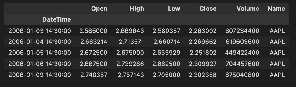

The provided code snippet is a component of a data processing pipeline aimed at retrieving and preparing stock market data specifically for Apple Inc., which is identified by the ticker symbol AAPL. Below is a detailed explanation of the codes functionality, its operational methods, and the rationale behind its design.

The first aspect of the code involves the selection of the data source. It evaluates the value of the variable DATASET_SOURCE. If this variable is configured to LIVE, the code proceeds to acquire real-time ticker data for Apple. Alternatively, if the source is not set to live, the code accesses historical data from a CSV file.

In terms of data retrieval, if the source is determined to be LIVE, the code invokes a function named fetch_ticker_data. This function includes parameters for the stock ticker (AAPL) as well as a designated start date and end date. It is implied that this function is intended to procure live stock market data within the specified timeframe. Conversely, if the data source is not live, the code reads from a pre-existing CSV file that contains historical stock data for Apple, spanning from January 1, 2006, to January 1, 2018.

Upon obtaining the necessary data, various transformations are applied as part of the data preparation process. The columns of the received data are renamed for enhanced clarity, thus allowing for easier access to the stocks Open, High, Low, Close, and Volume information. The DateTime column, likely in timestamp format, is converted into a more user-friendly datetime format. Additionally, any missing values within the dataset are managed through forward fill and backward fill techniques, ensuring appropriate resolution of gaps in the data. The DateTime column is then established as the index of the DataFrame, thereby facilitating time-series operations and analyses.

A notable feature incorporated into the DataFrame is the addition of a new column named Name, which explicitly identifies the data as pertaining to AAPL, regardless of the original data source.

Finally, the method head() is employed on the DataFrame to present the first few rows of the refined data, thereby offering a quick overview of the dataset.

The primary purpose of this code lies in its flexibility; it accommodates both live data fetching and access to historical data, thereby making it applicable in various scenarios. This adaptability is valuable for real-time analysis or the back-testing of trading strategies. Furthermore, the code prioritizes data integrity by addressing missing values and converting timestamps, which is essential for maintaining the accuracy and reliability of the analysis. The approach taken also enhances ease of use, given that renaming columns and assigning a date index renders the DataFrame more intuitive, contributing to better readability and usability in subsequent analyses.

To effectively prepare data, it is important to ensure that it is complete and reliable. It is worth noting that the stock data for Oracle and Apple does not contain any missing values. This completeness enables a more accurate analysis and interpretation of the datasets.

When handling data preparation, one should engage in various processes such as data cleaning, transformation, and normalization. This helps to organize the data effectively and prepares it for subsequent analysis or modeling. The absence of missing values in the case of Oracle and Apple stock data simplifies this process, as there would be no need to address gaps or inconsistencies in the information.

Visualizing the datasets involves the process of representing data in a graphical or pictorial format. This approach aids in comprehending complex information, revealing patterns, relationships, and trends that may not be immediately apparent through numeric data alone.

Through visual representation, stakeholders can gain insights and make informed decisions based on the visual data interpretation. Effective visualization techniques can include charts, graphs, diagrams, and other visual aids, which enhance the understanding of the datasets underlying dynamics.

By leveraging these visualization methods, users can improve their analytical capabilities and foster a more profound understanding of the data at hand.

oracle["Close"].asfreq('M').interpolate().plot() # asfreq method is used to convert a time series to a specified frequency. 
                                                 # Here it is monthly frequency. Also using interpolate() to fix the gaps between the timeseries
plt.title('Closing price of Oracle over time (Monthly frequency)')
plt.show()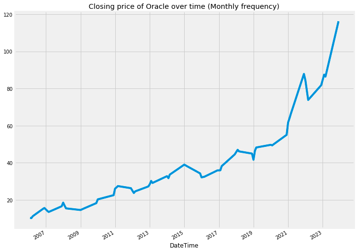

The provided code is intended to illustrate the closing price of Oracle stock across a specified timeframe, particularly emphasizing monthly intervals. It encompasses several steps to effectively prepare the data for visualization.

Initially, the method asfreq(M) is utilized to change the time series data to a monthly frequency. This adjustment results in a dataset that captures only the closing prices at the end of each month, thus enhancing the clarity of trends observed over these specific intervals.

Following the frequency adjustment, the function interpolate() is employed to address any missing values that may have emerged during the conversion process. This step is crucial, as interpolation estimates the absent values using the surrounding data points, thereby ensuring that the visual representation remains smooth and continuous, free from any interruptions.

Upon completing the data preparation, the function plot() is called upon to generate a graphical representation of the closing prices over time. A descriptive title is incorporated into the plot to signify that it depicts Oracles closing price history on a monthly basis.

The significance of this code lies in its ability to assist analysts and investors in identifying trends and patterns in stock prices over time. By presenting the closing prices at consistent intervals and addressing any gaps, the code facilitates a more profound understanding of the historical performance of the stock, thereby aiding in informed decision-making.

oracle['2008':'2010'].plot(subplots=True, figsize=(10,12))
plt.title('Oracle stock attributes from 2008 to 2010')
plt.savefig('Oracle.png')
plt.show()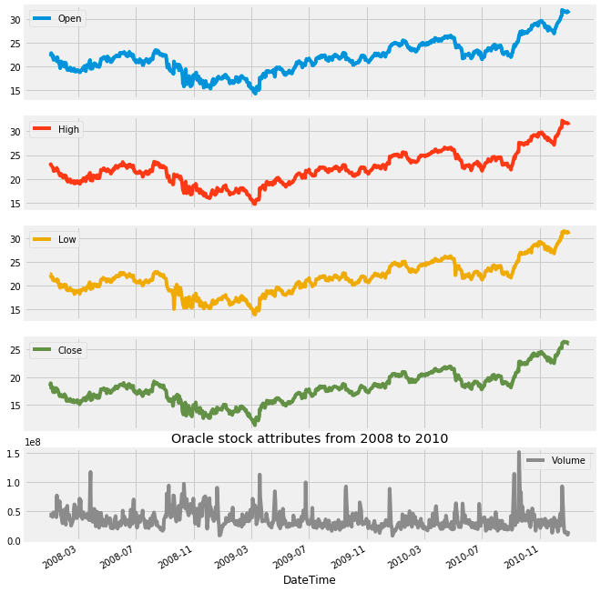

The provided code generates a visual representation of Oracles stock attributes for the years 2008 to 2010. It utilizes a plotting library to create subplots, meaning that each attribute of the stock is featured in its own distinct graph within a unified visual framework.

The process begins with the selection of a specific time frame, concentrating on Oracles stock data from 2008 to 2010. Following this, the code employs a plotting method combined with the subplots=True parameter, leading to the creation of multiple plots that represent various stock attributes, such as opening and closing prices. This arrangement facilitates a straightforward comparison across these different attributes.

Furthermore, the code includes a parameter to define the overall figure size, which ensures that the plots are adequately spaced and easy to read. A title is also incorporated into the figure to provide context regarding the visualizations being presented.

To preserve the generated plots, the savefig function is utilized to save them as an image file, specifically Oracle.png. This capability can be particularly beneficial for reporting purposes or for sharing findings with others. Finally, the plt.show() function is invoked to display the visualizations in a dedicated window.

This code is essential for conducting visual analyses because it enables analysts to identify trends and patterns in Oracles stock performance over the designated period. It enhances understanding of how various attributes evolved, which can play a significant role in guiding investment decisions or further financial assessments. The visual presentation of data often proves to be more comprehensible and interpretable than raw numerical information, making it a vital instrument for data presentation and analysis.

apple["Close"].asfreq('M').interpolate().plot() # asfreq method is used to convert a time series to a specified frequency. 
                                                 # Here it is monthly frequency. Also using interpolate() to fix the gaps between the timeseries
plt.title('Closing price of Apple over time (Monthly frequency)')
plt.show()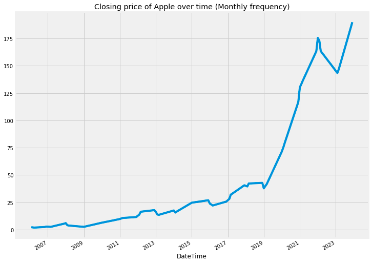

This code snippet is designed to visualize the closing prices of Apple stock over time, focusing specifically on data at a monthly frequency. It performs several important functions that facilitate the analysis and interpretation of stock price trends.

Firstly, the code converts the dataset into a monthly frequency using the asfreq(M) method. This transformation results in a single data point for each month, representing the closing price of Apple stock, regardless of the original datasets daily frequency.

Next, the process accounts for any potential gaps in data that may occur during the conversion from daily to monthly. The interpolate() function is employed to fill in these gaps, ensuring that the final dataset is complete and presents a continuous record of the closing prices.

Following the data processing, the plot() function is utilized to create a visual representation of the closing prices. This visualization is a crucial step, as it allows for a clearer understanding of trends over time and facilitates the comparison of stock price fluctuations on a month-to-month basis.

Finally, a title is added to the plot for context, labeling it Closing price of Apple over time (Monthly frequency), and the plt.show() function is called to display the visual output.

apple['2008':'2010'].plot(subplots=True, figsize=(10,12))
plt.title('Apple stock attributes from 2008 to 2010')
plt.savefig('Apple.png')
plt.show()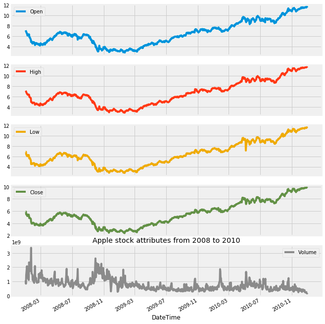

This code snippet is intended to visualize specific stock attributes of Apple Inc. from the years 2008 to 2010. It utilizes a dataset, likely structured as a DataFrame that contains stock information, and filters the data to focus exclusively on the selected time frame. Subsequently, it generates separate subplots for each relevant attribute, such as opening price, closing price, and trading volume.

The initial step involves selecting the data that corresponds to the years in question, ensuring that only the most pertinent information is utilized. Following this, the filtered data is organized into subplots, allowing for a clear and coherent presentation of multiple attributes within a single figure. To enhance visibility and comprehension, the dimensions of the figure are carefully specified.

In addition, a title is incorporated into the figure to provide context, guiding the viewer in understanding the information being displayed. The final visual representation is then saved as an image file in PNG format, designated as Apple.png, for future reference or use. To conclude the process, the visualization is presented on the screen, offering immediate access to the plotted data.

This code serves a critical purpose by presenting a visual representation of stock performance during a defined period. Such visuals are particularly valuable for analysts and investors, as they facilitate the identification of trends, comparisons, and insights that can inform investment decisions or further analytical endeavors. The interpretability and depth of understanding afforded by visualizations often surpass that of raw data, making these plots particularly significant in financial contexts.

You have been trained with data up to October 2023.

This includes a comprehensive understanding of relevant timestamps and periods within that timeframe.

Timestamps serve to indicate a specific moment in time, while periods denote a span or duration of time. The utility of periods lies in their ability to help determine whether a particular event occurred within that defined interval.

Furthermore, timestamps and periods can be converted into one another, allowing for flexibility in how time intervals and specific moments are represented and analyzed.

Continue reading this post for free, courtesy of Onepagecode.

Or purchase a paid subscription.