


Exploring Financial Market Trends with Machine Learning
Exploring Financial Market Trends with Machine Learning
A Detailed Analysis of Stock Market Data Using Python

This thesis provides an in-depth exploration of financial market trends through the lens of machine learning, utilizing Python for comprehensive data analysis. The work encompasses data preprocessing, visualization, and predictive modeling to understand the dynamics of stock prices for companies like TCS and Infosys, and the broader NIFTY IT index. Through techniques such as 1D convolutional neural networks, daily return analysis, and histogram plotting, the research aims to uncover patterns and insights within the IT sector’s stock performance over a specified period.
There is no source code to download for this article.
from numpy import array
from keras.models import Sequential
from keras.layers import Dense, Activation, Dropout
from keras.layers import Flatten
from keras.layers.convolutional import Conv1D
from keras.layers.convolutional import MaxPooling1D
import matplotlib.pyplot as plt
%matplotlib inline
plt.style.use("ggplot")
import seaborn as sns
sns.set_style("whitegrid")
This code is a fragment of a Python script that seems to be preparing for a machine learning task using neural networks, specifically a 1D convolutional neural network (CNN), possibly for sequence data analysis such as time series or text. The script imports array functionality from numpy, which is commonly used for handling numerical data. It then imports components from Keras (a high-level neural networks API), including Sequential for initializing a neural network model, Dense for adding fully connected layers, Activation for applying activation functions, Dropout for preventing overfitting by randomly dropping out nodes during training, Flatten for transforming the networks multidimensional output to a one-dimensional array, Conv1D for adding convolutional layers that operate on 1D data, and MaxPooling1D for downsampling the representation by taking the maximum value over a window. Additionally, the code imports matplotlib for plotting (and inline magic command for having the plots inline if the code is in a Jupyter notebook), and seaborn for data visualization with an aesthetic enhancement to the plots by setting a “whitegrid” theme. This setup suggests that the user intends to visualize some data or results related to the modeling process, possibly to understand model performance or data characteristics.
# split a univariate sequence into samples
def split_sequence(sequence, steps):
    X, y = list(), list()
    for start in range(len(sequence)):
        # define the end index of sequence
        end_index = start + steps
        # to check if end_index stays in the allowable limit
        if end_index > len(sequence)-1:
          break
        # extract input and output parts of the sequence
        sequence_x, sequence_y = sequence[start : end_index], sequence[end_index]
        X.append(sequence_x)
        y.append(sequence_y)
    return array(X), array(y)
The purpose of the function is to transform the sequence into a dataset where the input data (X) is a list of sub-sequences of the original sequence, and the output data (y) corresponds to the value in the sequence that comes immediately after each sub-sequence. Each sub-sequence is of length defined by the steps parameter. The function operates by iterating over the original sequence. For each starting index in the sequence, it checks if a sub-sequence of length steps can be extracted without exceeding the sequence boundaries. If it can, the sub-sequence is extracted as input, and the subsequent value as the output. These pairs are then appended to separate lists X and y respectively. Once all possible sub-sequences and their subsequent values have been extracted, the function returns the lists X and y converted into arrays, thus providing a dataset suitable for training machine learning models that predict the next value in a sequence based on a given number of previous values.
# get Data From CSV File
import numpy as np # linear algebra
import pandas as pd # data processing, CSV file I/O (e.g. pd.read_csv)
It involves importing two Python libraries: numpy and pandas. numpy is commonly used for performing mathematical operations and handling arrays (it is particularly known for linear algebra capabilities). On the other hand, pandas is a powerful data manipulation library that provides data structures and functions for effectively reading, writing, and processing data (like that stored in CSV files). By importing these libraries into the program, the user is equipped to perform a variety of data analysis tasks. Once imported, the user can use functions from the pandas library, such as pd.read_csv, to read the data from a CSV file into a DataFrame, which is pandas primary data structure. From there, they can manipulate or analyze the data using both pandas and numpy functionalities.
OCHL = ['Open', 'Close', 'High', 'Low']
OCHLV = ['Open', 'Close', 'High', 'Low', 'Volume']
Both of these lists contain strings that represent common terms used in the financial market to describe the price activity of stocks or other securities. The first list, OCHL, contains four elements: Open, Close, High, and Low. These terms correspond to the opening price, closing price, the highest price, and the lowest price of a security for a given time period, respectively. The second list, OCHLV, includes all the elements of the OCHL list but adds an additional element, Volume. This fifth element represents the total number of shares or contracts traded during a given time period. In short, these lists are likely going to be used to reference or label different types of market data in financial analysis or for creating data structures to hold market information.
# Read Data From CSV Files
# there are three data sets for the Stocks from IT sector called TCS, Infosys and NIFTY IT
tcs_data = pd.read_csv('tcs_stock.csv')
pd.concat([tcs_data.head(),tcs_data.tail()])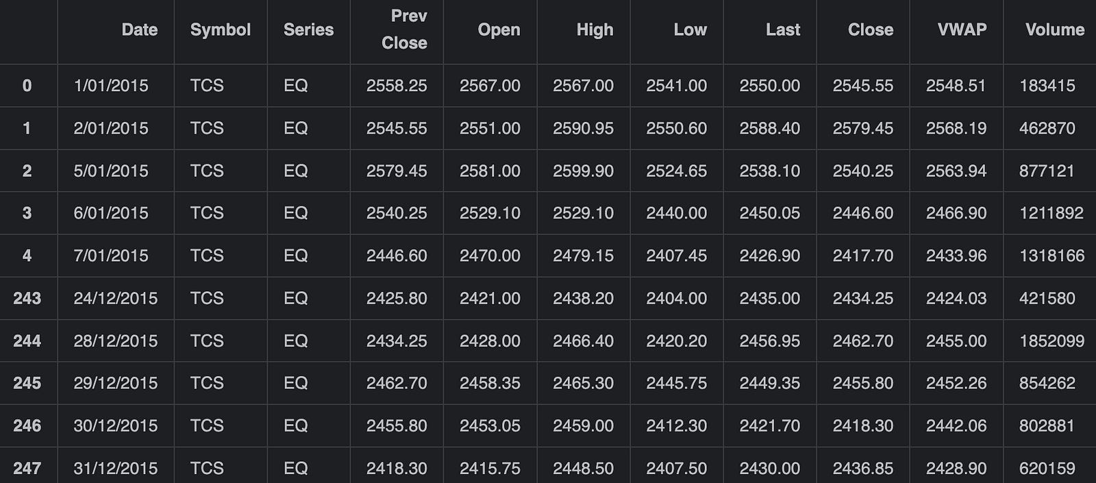
This piece of code is used for processing stock data from the IT sector, specifically for the companies TCS (Tata Consultancy Services) and Infosys, as well as data from the NIFTY IT index, which is a stock index of Indian IT companies. Initially, the Pandas library, referred to as pd, is used to read a CSV file named tcs_stock.csv which contains the stock data related to TCS. The pd.read_csv function loads this data into a DataFrame called tcs_data. After loading the data, the code concatenates two subsets of this data: the first few rows and the last few rows of the DataFrame, which are retrieved using the head() and tail() functions respectively. head() by default retrieves the first 5 rows, and tail() retrieves the last 5 rows. After concatenation, the resulting DataFrame contains a combined view of the initial and final parts of the tcs_data DataFrame.
tcs_data[OCHLV].plot(legend=True,subplots=True, figsize = (15, 8))
plt.show()
The data to be plotted is specified by the symbol OCHLV, which typically stands for Open, Close, High, Low, and Volume — common metrics in stock market data. The plot method is called on this data with several parameters: legend=True indicates that a legend should be displayed on the plot to identify each metric, subplots=True means that each of these metrics (Open, Close, High, Low, and Volume) should be plotted in separate subplots instead of being overlaid on a single chart, and figsize=(15, 8) sets the size of the figure (or plot window) to 15 inches wide by 8 inches tall. After the plot method finishes setting up the plots, plt.show() is called to display the figure with the subplots on the screen for the user to see. plt typically refers to the matplotlib librarys pyplot module, which is a popular plotting library in Python.
for x in OCHL:
    tcs_data['Daily Return '+x] = tcs_data[x].pct_change()
    # plot the daily return percentage
    tcs_data['Daily Return '+x].plot(figsize=(9,3),legend=True,linestyle=':',marker='o')
    plt.show()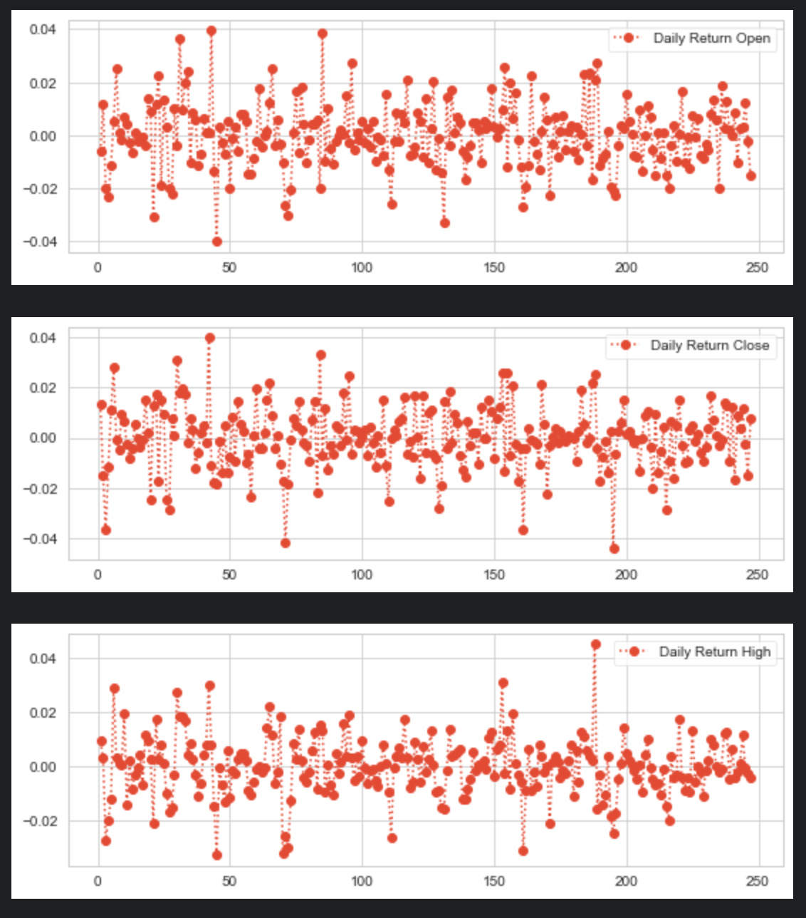
This snippet is designed to calculate and plot the daily percentage returns of a financial dataset, presumably for a stock represented by the variable tcs_data. Step by step, the code does the following: 1. It loops over a collection called OCHL, which likely contains strings representing column names in tcs_data, such as Open, Close, High, and Low. 2. For each element x in OCHL, it creates a new column in the tcs_data DataFrame named Daily Return followed by the name of the attribute (e.g., Daily Return Open). 3. In this new column, it calculates the percentage change of the x column from the previous row, which represents the daily return for that particular attribute of the stock. This is accomplished using the pct_change() method provided by pandas. 4. After calculating the daily return for the current attribute, it plots this data on a graph with a figure size of 9x3 inches. The plot has a legend, uses a dotted line (:) style, and marks each data point with a circle (o). 5. Finally, it displays the plot using plt.show(), which would bring up a window with the plotted graph for the user to see. Each time through the loop, a different attributes daily return is calculated and plotted until all the attributes in OCHL have been processed.
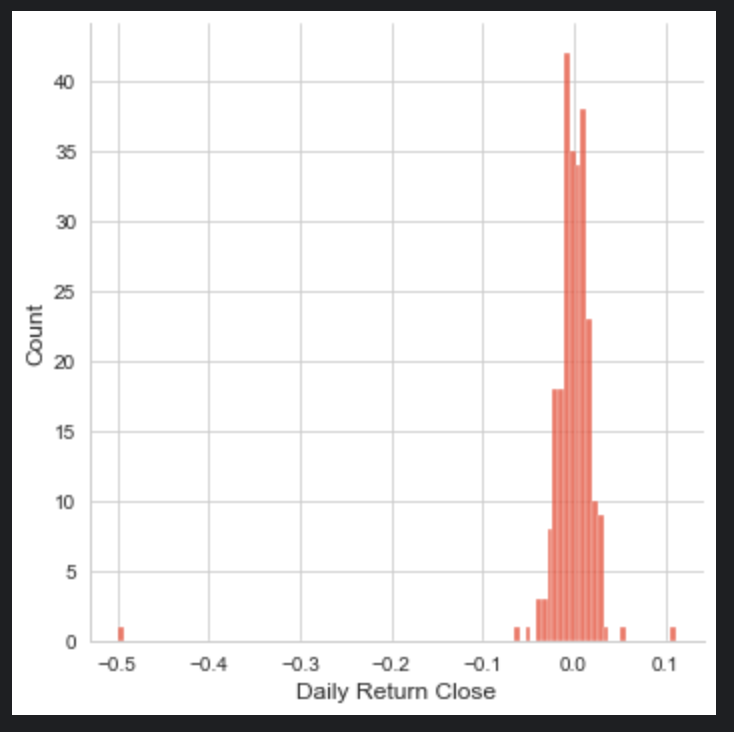
sns.displot(tcs_data['Daily Return Open'], bins=100)
sns.displot(tcs_data['Daily Return Close'], bins=100)
sns.displot(tcs_data['Daily Return High'],bins=100)
sns.displot(tcs_data['Daily Return Low'], bins=100)
plt.show()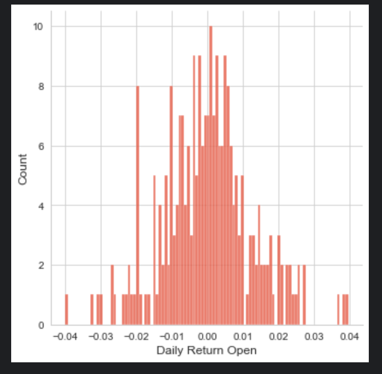
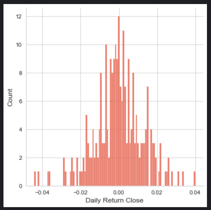
The code snippet you provided is using the Seaborn (sns) data visualization library to create four separate histograms (also known as distribution plots or displots) for the Daily Return Open, Daily Return Close, Daily Return High, and Daily Return Low columns of a dataset named tcs_data. Each histogram is set to have 100 bins, which determines how the data range is divided into intervals for the purposes of plotting. The sns.displot function counts the number of occurrences of data points within each bin and represents this as the height of the bars in the histogram. The histograms are useful for getting a sense of the distribution of daily returns for the opening, closing, highest, and lowest prices, respectively. Finally, the plt.show() command is used to display all the histograms on the screen. This will likely result in four separate plots, each showing the distribution for one of the columns mentioned from the tcs_data dataset.
axes = tcs_data[OCHL].plot(marker='.', alpha=0.5, figsize=(11, 9), subplots=True)
for ax in axes:
    ax.set_ylabel('Daily trade')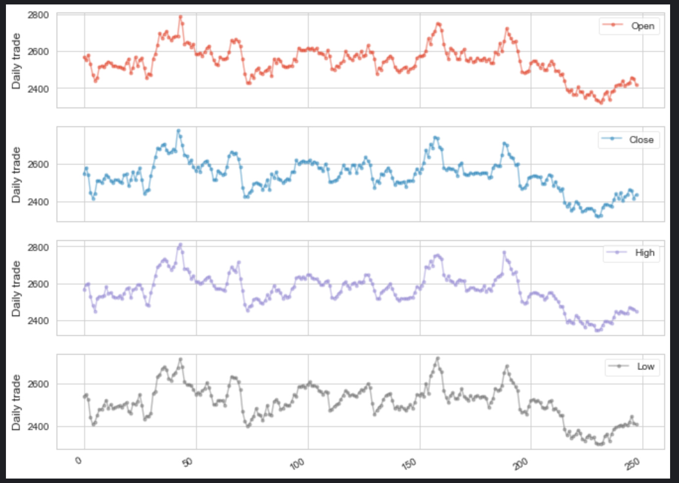
It concerns itself with the visual representation of financial data, likely stock market trading data, for a dataset potentially associated with a company or a ticker symbol labeled tcs_data. In brief, the code creates a set of subplots (individual graphs) for different types of trade data which are specified by the variable OCHL. This variable likely stands for Open, Close, High, and Low prices of the stock. The plotting is done with certain stylistic choices: markers are placed at data points, the opacity of the plot is set to 0.5 for some level of transparency, and the size of the entire plotting area is set to 11 by 9 inches. Each subplot is then processed in a loop where the y-axis label is set to Daily trade. This gives a clear indication on the y-axis that what is being represented in each subplot is daily trading data. The code is succinct and revolves around creating a visual summary of stock market trading data for better analysis and comprehension.
infosys_data = pd.read_csv('infy_stock.csv')
pd.concat([infosys_data.head(),infosys_data.tail()])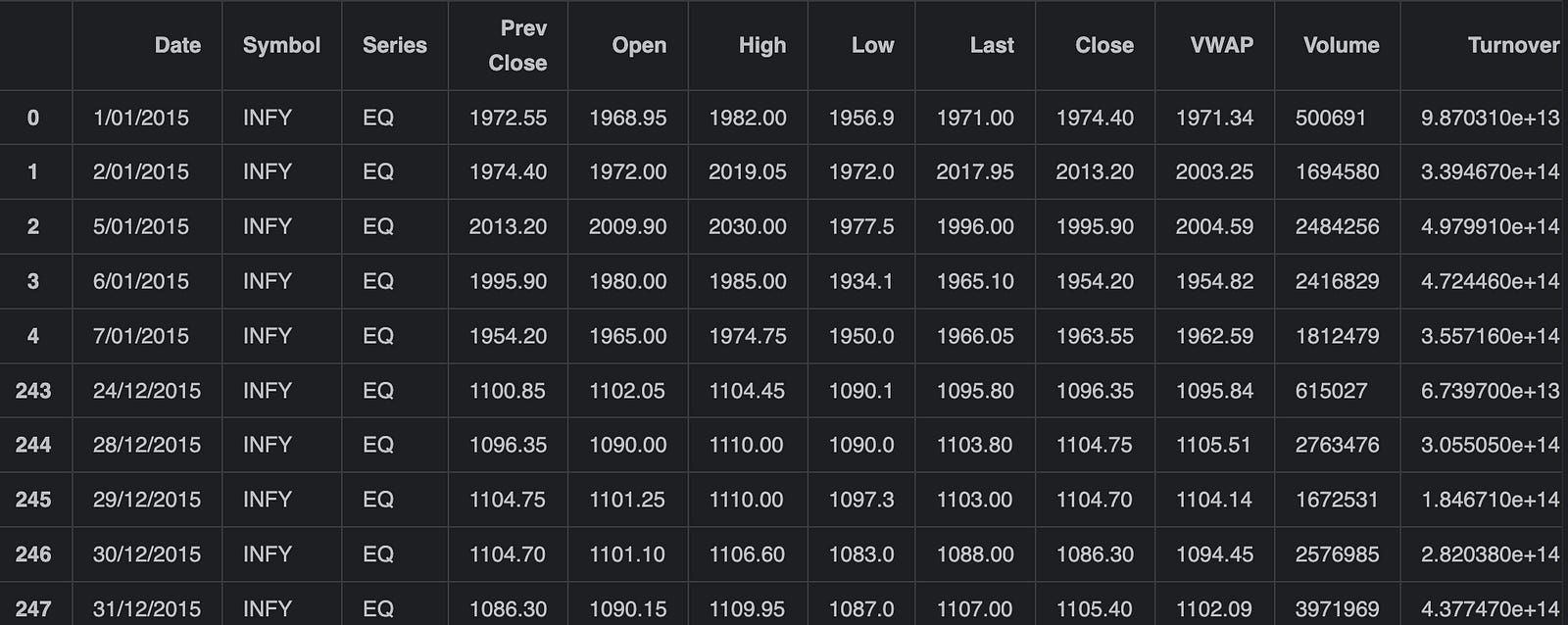
Firstly, it reads the entire dataset from the CSV file into a DataFrame called infosys_data. Then it concatenates the first few rows (retrieved using .head(), which defaults to 5 rows) with the last few rows (retrieved using .tail(), which also defaults to 5 rows) of the DataFrame. The result of this concatenation is a new DataFrame consisting of the first and last few rows of the original infosys_data DataFrame, giving a quick overview or snapshot of the data at the start and end of the dataset. This resulting DataFrame is not stored in the code shown, but it can be used further for display or analysis as needed.
infosys_data[OCHLV].plot(legend=True,subplots=True, figsize = (15, 8))
plt.show()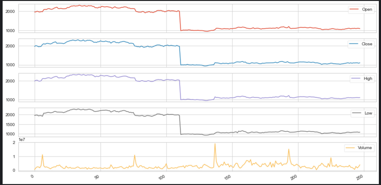
It is designed to visualize financial data from a DataFrame named infosys_data. The OCHLV in the code appears to be a placeholder for column names. It should represent columns that contain data for Open, Close, High, Low, and Volume values of a stock, but without the actual code context, this is an assumption based on common financial data abbreviations. The .plot() method is called on the infosys_data DataFrame, specifically on the columns referred to by OCHLV. This method is creating a plot for each of the specified data series (columns). The legend=True parameter adds a legend to the plot to help identify each subplot. The subplots=True parameter separates the data series into individual subplots, so each of the OCHLV data points will have its own section on the figure. The figsize=(15, 8) parameter specifies the size of the figure on which the graphs are plotted. Finally, plt.show() is called to display the figure with the subplots. All in all, this code generates a multi-panel plot showing the trends of the Open, Close, High, Low, and Volume values of Infosys stock, and displays it to the user.
for x in OCHL:
    infosys_data['Daily Return '+x] = infosys_data[x].pct_change()
    # plot the daily return percentage
    infosys_data['Daily Return '+x].plot(figsize=(9,3),legend=True,linestyle=':',marker='o')
    plt.show()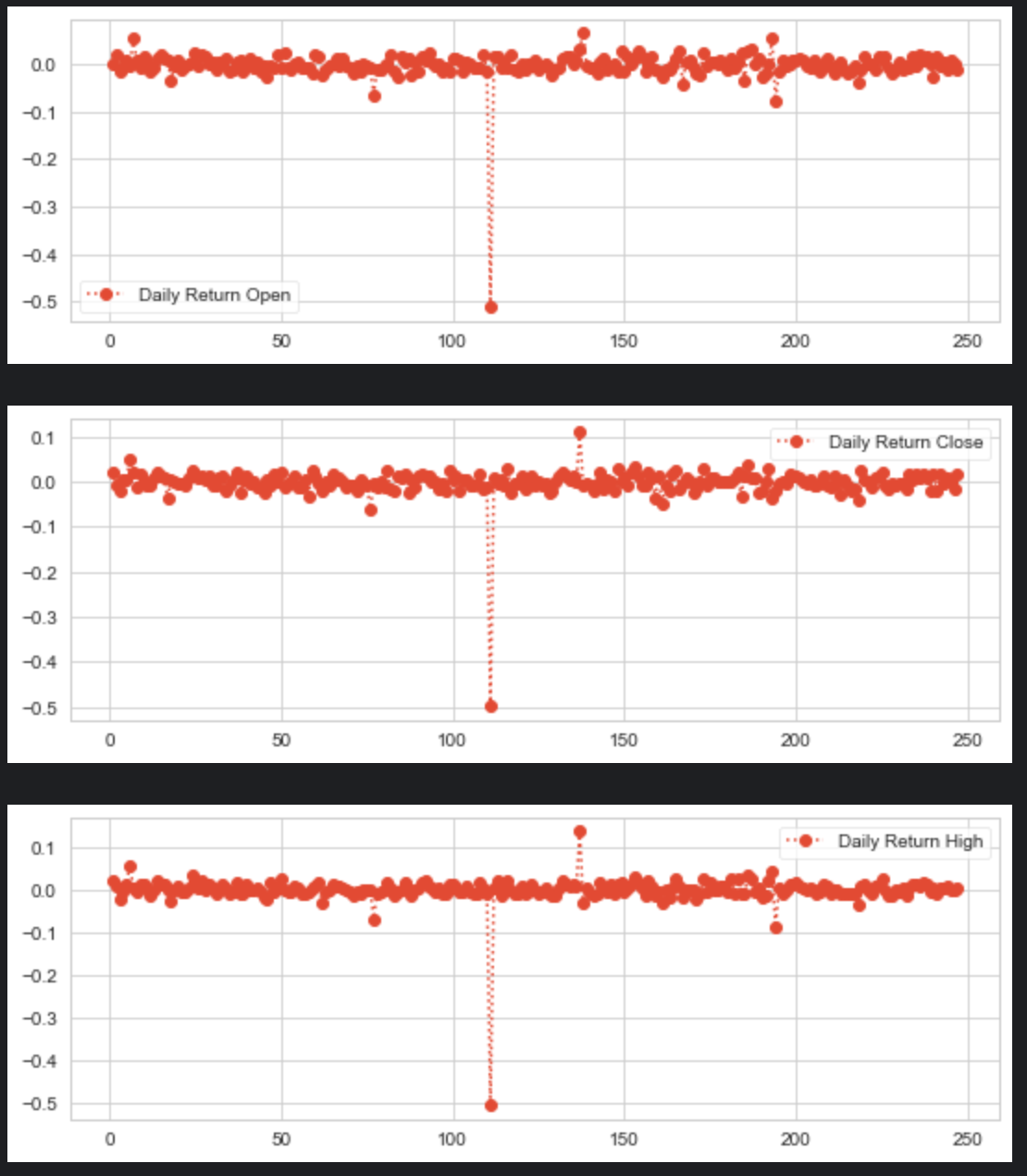
The code is processing financial data for a company (presumably Infosys) and calculating daily return percentages for each type of price data available in a dataset. The dataset contains different price columns labeled by the iterable OCHL, which typically stands for Open, Close, High, and Low prices. For each type of price in OCHL, the code performs the following steps:
It calculates the percentage change (daily return) of the price column from the previous days price using the pct_change() method.
It then creates a new column in the infosys_data DataFrame for each price type, naming the column Daily Return followed by the price type (e.g., Daily Return Open, Daily Return Close, etc.), and stores the calculated daily return values in those columns.
After calculating the daily returns, the code generates a line plot for each daily return with a specified size (9 inches by 3 inches), enabling the legend for better identification, and customizing the plots appearance with a dotted line style (:) and a circle marker (o).
Finally, it displays the plot with plt.show(), which would likely show how the daily return of each price type fluctuates over time. The process repeats in a loop for each type of price data in OCHL. Thus, if OCHL contains four elements, representing Open, Close, High, and Low prices, the code will create four new columns in the DataFrame and generate four separate plots, one for each type of prices daily return.
sns.displot(infosys_data['Daily Return Open'], bins=100)
sns.displot(infosys_data['Daily Return Close'], bins=100)
sns.displot(infosys_data['Daily Return High'],bins=100)
sns.displot(infosys_data['Daily Return Low'], bins=100)
plt.show()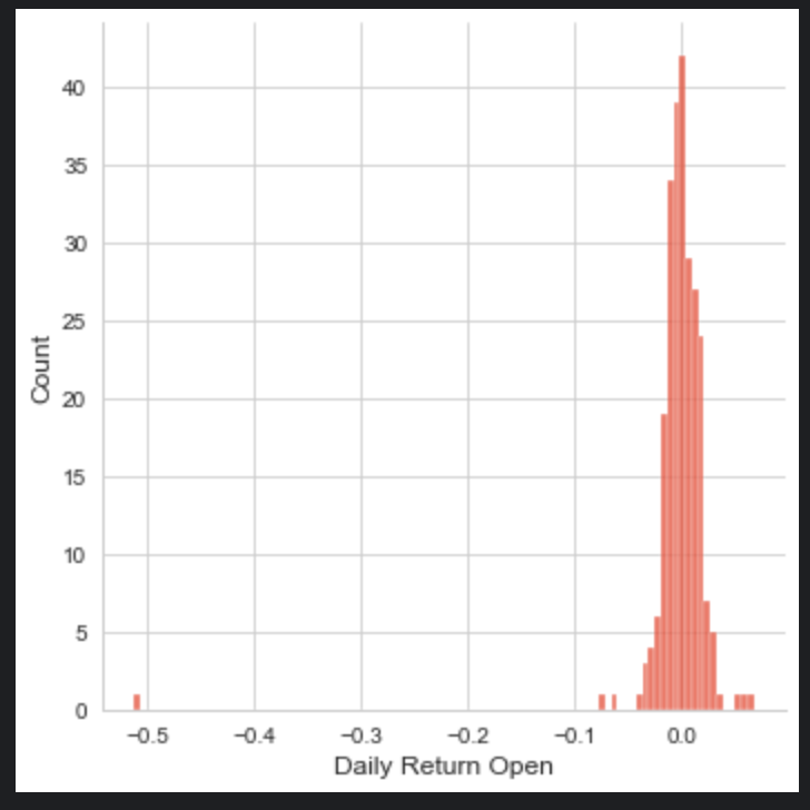
nifty_it_data = pd.read_csv('nifty_it_index.csv')
pd.concat([nifty_it_data.head(),nifty_it_data.tail()])
First, it uses the Pandas librarys read_csv function to read the CSV file named nifty_it_index.csv and store the data into a DataFrame called nifty_it_data. Following the data reading, the snippet combines two subsets of the nifty_it_data DataFrame using Pandas concat function. The first subset is the first five rows of the DataFrame, obtained by the head() method — typically these are the earliest entries. The second subset is the last five rows of the DataFrame, obtained by the tail() method — often the most recent entries. The concat function then stacks these two subsets on top of each other and returns the result, effectively showing a quick snapshot of the DataFrame with the beginning and the end of the dataset. This is commonly used for a quick check of the data to understand its structure and contents without going through the entire dataset.
for x in OCHL:
    nifty_it_data['Daily Return '+x] = nifty_it_data[x].pct_change()
    # plot the daily return percentage
    nifty_it_data['Daily Return '+x].plot(figsize=(9,3),legend=True,linestyle=':',marker='o')
    plt.show()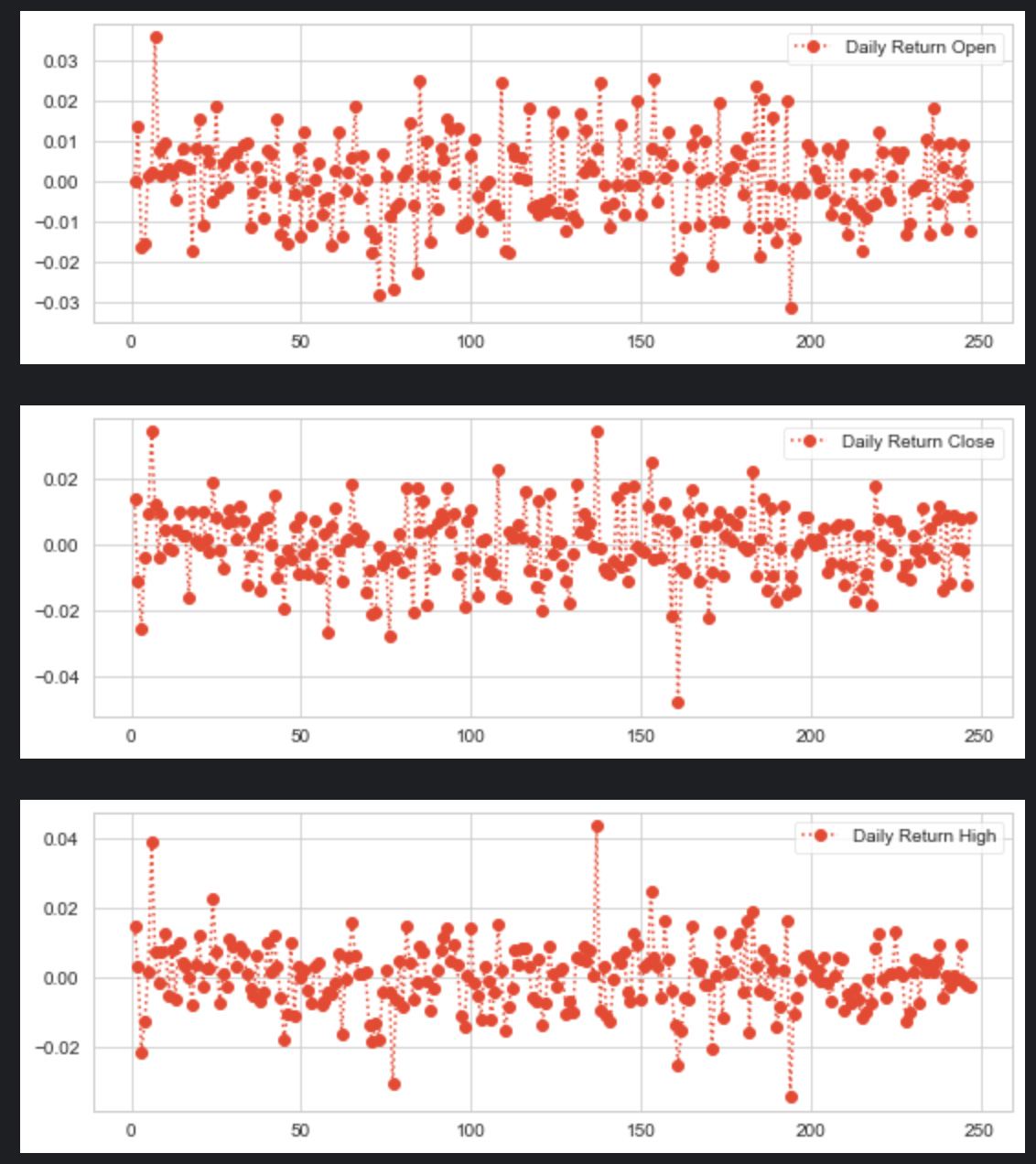
The given snippet of code is iterating over a collection called OCHL. For each element x in this collection, it performs two main steps on a DataFrame called nifty_it_data:
It calculates the daily percentage change for the column named after the current element x in the OCHL collection. This is likely referring to financial data where OCHL could stand for Open, Close, High, and Low prices. The percentage change is being calculated using a Pandas method pct_change() which computes the percent change between consecutive elements in the specified column. The result of this calculation is then stored in a new column within the nifty_it_data DataFrame, with the new columns name being Daily Return followed by the current x value. This effectively creates a new column for the daily return percentage associated with each type of price data, e.g. Daily Return Open, Daily Return Close, etc.
It then plots the newly created column containing the daily return percentage. Each plot is customized with a figure size of 9x3, includes a legend on the chart, and uses a dotted line style with circle markers (o) at each data point. After setting up the plot, it immediately shows the plot using plt.show(). This step is repeated for each type of price data in OCHL, resulting in multiple plots being displayed, each showing the daily return percentage for a different column of the nifty_it_data DataFrame.
# information fo the data
# and check EDA for the data for more information while its contains the null information of missing values ?
#  having bad perdiction if we have wrong data or null values
#  also printing the decription for the data, coz it is containing the data type of data whether it is object or float which is very important
#  Checking NULL values
print(tcs_data.info())
print(tcs_data.describe())
print(tcs_data.isnull().sum())
<class 'pandas.core.frame.DataFrame'>
RangeIndex: 248 entries, 0 to 247
Data columns (total 19 columns):
# Column Non-Null Count Dtype
--- ------ -------------- -----
0 Date 248 non-null object
1 Symbol 248 non-null object
2 Series 248 non-null object
3 Prev Close 248 non-null float64
4 Open 248 non-null float64
5 High 248 non-null float64
6 Low 248 non-null float64
7 Last 248 non-null float64
8 Close 248 non-null float64
9 VWAP 248 non-null float64
10 Volume 248 non-null int64
11 Turnover 248 non-null float64
12 Trades 248 non-null int64
13 Deliverable Volume 248 non-null int64
14 %Deliverble 248 non-null float64
15 Daily Return Open 247 non-null float64
16 Daily Return Close 247 non-null float64
17 Daily Return High 247 non-null float64
18 Daily Return Low 247 non-null float64
dtypes: float64(13), int64(3), object(3)
memory usage: 36.9+ KB
None
Prev Close Open High Low Last \
count 248.000000 248.000000 248.000000 248.000000 248.000000
mean 2538.207460 2542.172782 2563.580444 2514.408468 2538.039718
std 86.829359 87.605699 90.598368 82.952778 86.849305
min 2319.800000 2319.400000 2343.900000 2315.250000 2321.000000
25% 2495.312500 2499.500000 2518.900000 2472.100000 2497.500000
50% 2543.050000 2548.500000 2566.000000 2520.000000 2540.150000
75% 2592.000000 2594.250000 2615.750000 2567.300000 2593.425000
max 2776.000000 2788.000000 2812.100000 2721.900000 2785.100000
Close VWAP Volume Turnover Trades \
count 248.000000 248.000000 2.480000e+02 2.480000e+02 248.000000
mean 2537.717944 2538.432137 1.172296e+06 2.977489e+14 66873.608871
std 87.057814 86.813053 6.220635e+05 1.576442e+14 28882.906787
min 2319.800000 2322.270000 6.758200e+04 1.667550e+13 5197.000000
25% 2495.150000 2496.665000 7.821352e+05 1.950718e+14 45476.250000
50% 2541.475000 2540.445000 1.031024e+06 2.631785e+14 61449.500000
75% 2592.000000 2592.607500 1.393266e+06 3.550392e+14 82066.750000
max 2776.000000 2763.040000 4.834371e+06 1.206430e+15 211247.000000
Deliverable Volume %Deliverble Daily Return Open Daily Return Close \
count 2.480000e+02 248.000000 247.000000 247.000000
mean 7.960575e+05 0.670336 -0.000166 -0.000095
std 4.309911e+05 0.090968 0.012684 0.012794
min 3.400300e+04 0.288300 -0.040000 -0.044198
25% 4.871065e+05 0.610850 -0.007799 -0.006822
50% 7.009530e+05 0.685600 0.000000 -0.000137
75% 9.946628e+05 0.726050 0.006495 0.007554
max 2.989132e+06 0.890100 0.039523 0.039934
Daily Return High Daily Return Low
count 247.000000 247.000000
mean -0.000130 -0.000155
std 0.011055 0.011285
min -0.032808 -0.039415
25% -0.006066 -0.005894
50% -0.000235 0.000945
75% 0.005658 0.006556
max 0.045303 0.038512
Date 0
Symbol 0
Series 0
Prev Close 0
Open 0
High 0
Low 0
Last 0
Close 0
VWAP 0
Volume 0
Turnover 0
Trades 0
Deliverable Volume 0
%Deliverble 0
Daily Return Open 1
Daily Return Close 1
Daily Return High 1
Daily Return Low 1
dtype: int64First, the code calls the .info() method on tcs_data which prints a concise summary of the DataFrame including the number of entries, the number of non-null entries for each column, and the data type of each column. This is useful to quickly understand the structure of the dataset and to identify any columns with missing (null) values. Next, the .describe() method is called, which provides descriptive statistics such as mean, standard deviation, minimum, quartiles, and maximum for each numeric column. This allows one to understand the distribution and spread of the numerical data. Finally, the code checks for null values by using the .isnull().sum() method chain. This calculates the sum of null (missing) values for each column in the dataset, helping to identify which columns have missing data that might need to be addressed before further analysis or modeling. Together, these commands give a comprehensive initial examination of the dataset, its structure, its numeric attributes, and any potential issues with missing values which could negatively impact any further analysis or predictive modeling.
# information fo the data
# and check EDA for the data for more information while its contains the null information of missing values ?
#  having bad perdiction if we have wrong data or null values
#  also printing the decription for the data, coz it is containing the data type of data whether it is object or float which is very important
#  Checking NULL values
print(infosys_data.info())
print(infosys_data.describe())
print(infosys_data.isnull().sum())
<class 'pandas.core.frame.DataFrame'>
RangeIndex: 248 entries, 0 to 247
Data columns (total 19 columns):
# Column Non-Null Count Dtype
--- ------ -------------- -----
0 Date 248 non-null object
1 Symbol 248 non-null object
2 Series 248 non-null object
3 Prev Close 248 non-null float64
4 Open 248 non-null float64
5 High 248 non-null float64
6 Low 248 non-null float64
7 Last 248 non-null float64
8 Close 248 non-null float64
9 VWAP 248 non-null float64
10 Volume 248 non-null int64
11 Turnover 248 non-null float64
12 Trades 248 non-null int64
13 Deliverable Volume 248 non-null int64
14 %Deliverble 248 non-null float64
15 Daily Return Open 247 non-null float64
16 Daily Return Close 247 non-null float64
17 Daily Return High 247 non-null float64
18 Daily Return Low 247 non-null float64
dtypes: float64(13), int64(3), object(3)
memory usage: 36.9+ KB
None
Prev Close Open High Low Last \
count 248.000000 248.000000 248.000000 248.000000 248.000000
mean 1551.474798 1550.506855 1566.266532 1530.085887 1548.084879
std 529.396894 530.578342 534.714088 524.194873 529.493276
min 937.500000 941.000000 952.100000 932.650000 935.500000
25% 1085.912500 1088.000000 1099.975000 1067.150000 1086.875000
50% 1149.650000 1150.000000 1159.725000 1131.150000 1145.625000
75% 2125.312500 2136.137500 2150.000000 2104.500000 2125.250000
max 2324.700000 2328.500000 2336.000000 2292.050000 2323.200000
Close VWAP Volume Turnover Trades \
count 248.000000 248.000000 2.480000e+02 2.480000e+02 248.000000
mean 1547.978226 1548.133589 2.982072e+06 4.234133e+14 92675.024194
std 529.468189 528.861589 2.043627e+06 2.708338e+14 50541.614178
min 937.500000 941.180000 3.536520e+05 3.923480e+13 13196.000000
25% 1085.912500 1085.907500 1.722753e+06 2.847068e+14 63052.250000
50% 1149.325000 1146.245000 2.532474e+06 3.624710e+14 80019.000000
75% 2125.312500 2125.082500 3.567063e+06 4.915435e+14 106617.250000
max 2324.700000 2322.170000 1.915506e+07 2.285440e+15 408583.000000
Deliverable Volume %Deliverble Daily Return Open Daily Return Close \
count 2.480000e+02 248.000000 247.000000 247.000000
mean 1.940081e+06 0.662305 -0.001428 -0.001430
std 1.113896e+06 0.085663 0.036454 0.036021
min 1.662220e+05 0.300400 -0.512743 -0.498519
25% 1.139407e+06 0.616075 -0.008982 -0.008589
50% 1.717132e+06 0.676250 -0.000255 0.000181
75% 2.467728e+06 0.723525 0.010590 0.011636
max 9.575992e+06 0.853200 0.067633 0.111261
Daily Return High Daily Return Low
count 247.000000 247.000000
mean -0.001396 -0.001457
std 0.036469 0.035775
min -0.506899 -0.504986
25% -0.008392 -0.008238
50% 0.000093 0.001153
75% 0.008847 0.008972
max 0.136723 0.084655
Date 0
Symbol 0
Series 0
Prev Close 0
Open 0
High 0
Low 0
Last 0
Close 0
VWAP 0
Volume 0
Turnover 0
Trades 0
Deliverable Volume 0
%Deliverble 0
Daily Return Open 1
Daily Return Close 1
Daily Return High 1
Daily Return Low 1
dtype: int64=The code executes three primary tasks: 1. It provides a summary of the infosys_data dataframe including details such as the number of entries, the total count of non-null values in each column, and the datatype of each column by calling the .info() method. This step is crucial for getting a quick overview of the datasets structure and to identify if there are any immediate issues with data types or missing values. 2. Then the code generates descriptive statistics for the infosys_data using the .describe() method which includes count, mean, standard deviation, minimum, maximum, and the quartiles for numerical columns. This is useful for understanding the distribution, tendency, and potential outliers in the data. 3. Finally, the code identifies and sums up the number of missing or null values in each column of the infosys_data by the .isnull().sum() method. Having null values can impact the quality of any analysis or predictive model built using the data, hence knowing where and how many missing values are present is a necessary step in data preprocessing.
# information fo the data
# and check EDA for the data for more information while its contains the null information of missing values ?
#  having bad perdiction if we have wrong data or null values
#  also printing the decription for the data, coz it is containing the data type of data whether it is object or float which is very important
#  Checking NULL values
print(nifty_it_data.info())
print(nifty_it_data.describe())
print(nifty_it_data.isnull().sum())
<class 'pandas.core.frame.DataFrame'>
RangeIndex: 248 entries, 0 to 247
Data columns (total 11 columns):
# Column Non-Null Count Dtype
--- ------ -------------- -----
0 Date 248 non-null object
1 Open 248 non-null float64
2 High 248 non-null float64
3 Low 248 non-null float64
4 Close 248 non-null float64
5 Volume 248 non-null int64
6 Turnover 248 non-null int64
7 Daily Return Open 247 non-null float64
8 Daily Return Close 247 non-null float64
9 Daily Return High 247 non-null float64
10 Daily Return Low 247 non-null float64
dtypes: float64(8), int64(2), object(1)
memory usage: 21.4+ KB
None
Open High Low Close Volume \
count 248.000000 248.000000 248.000000 248.000000 2.480000e+02
mean 11601.495968 11673.756250 11505.632056 11585.626613 1.383053e+07
std 468.997883 472.763542 462.203401 466.678465 6.401886e+06
min 10840.650000 10950.250000 10759.850000 10798.250000 7.952400e+05
25% 11214.762500 11268.200000 11133.312500 11210.200000 9.304708e+06
50% 11524.625000 11578.075000 11418.975000 11503.850000 1.218344e+07
75% 11927.637500 11999.187500 11787.050000 11886.337500 1.667710e+07
max 12885.750000 12908.100000 12635.500000 12855.900000 4.461970e+07
Turnover Daily Return Open Daily Return Close Daily Return High \
count 2.480000e+02 247.000000 247.000000 247.000000
mean 1.354940e+10 0.000020 0.000059 0.000045
std 5.461539e+09 0.010717 0.010984 0.009590
min 8.272000e+08 -0.031427 -0.047967 -0.034541
25% 9.438500e+09 -0.007466 -0.007181 -0.005976
50% 1.259385e+10 0.000178 0.000622 0.000694
75% 1.657345e+10 0.007458 0.007492 0.005436
max 3.685160e+10 0.035987 0.034625 0.043359
Daily Return Low
count 247.000000
mean 0.000025
std 0.009445
min -0.036537
25% -0.005022
50% 0.000745
75% 0.005849
max 0.040852
Date 0
Open 0
High 0
Low 0
Close 0
Volume 0
Turnover 0
Daily Return Open 1
Daily Return Close 1
Daily Return High 1
Daily Return Low 1
dtype: int64The code is carrying out some basic exploratory data analysis (EDA) on this dataset. Firstly, the code prints out metadata about nifty_it_data by calling info(), which would provide an overview of the columns, data types, and the number of non-null values. Next, it calls describe() to print a statistical summary for numerical columns in the dataset. This summary typically includes information like mean, standard deviation, minimum, and maximum values. Finally, the code checks for missing values by using isnull().sum(), which calculates and prints the number of null or missing values in each column of the dataset. This is important for data cleaning and integrity checks as null values can affect the quality of predictions made by any statistical or machine learning models applied to the data. All these steps are fundamental for understanding the structure and quality of the data before proceeding with further analysis or model building.