

Exploring Generative Adversarial Networks with PyTorch
Integrating GANs into Machine Learning Models

In the rapidly evolving world of artificial intelligence, Generative Adversarial Networks (GANs) stand out as a groundbreaking development, particularly in machine learning and image processing. This article offers a comprehensive exploration of GANs using PyTorch, a leading framework in the AI domain. Our focus is on practical implementation, leveraging the MNIST dataset to demonstrate the power and versatility of GANs.
We begin by setting up an interactive coding environment using Google Colab and Google Drive, ensuring a streamlined and efficient workflow. The journey through GANs encompasses the construction and fine-tuning of the two pivotal components of GANs: the generator and the discriminator. Accompanied by detailed code examples, we delve into the architectural intricacies of these networks, highlighting the role of various layers and activation functions. Alongside implementation, we also emphasize the importance of understanding and computing loss functions, crucial for the effectiveness of GAN models. Whether you are a budding enthusiast or a seasoned practitioner in AI, this guide offers valuable insights into the practical and theoretical aspects of GANs in Python.
# this mounts your Google Drive to the Colab VM.
from google.colab import drive
drive.mount('/content/drive', force_remount=True)

# enter the foldername in your Drive where you have saved the unzipped
# assignment folder, e.g. 'cs231n/assignments/assignment3/'
FOLDERNAME = 'cs231n/assignments/assignment3/'
assert FOLDERNAME is not None, "[!] Enter the foldername."

# now that we've mounted your Drive, this ensures that
# the Python interpreter of the Colab VM can load
# python files from within it.
import sys
sys.path.append('/content/drive/My Drive/{}'.format(FOLDERNAME))

# this downloads the CIFAR-10 dataset to your Drive
# if it doesn't already exist.
%cd drive/My\ Drive/$FOLDERNAME/cs231n/datasets/
!bash get_datasets.sh
%cd /content
An online platform for sharing and executing Python code, Google Colaboratory Colab, uses this Python code. We import the required package drive from the google.colab library, which allows Colab to access Google Drive. Using drive.mount, we mount Google Drive to the Colab virtual machine. Within our Colab notebook, we can access files and folders from Google Drive. As a next step, we specify the folder name in our Google Drive where the assignment folder has been saved. This allows us to access and work with the assignment files easily. A folder name cannot be empty using the assert statement.
In the Colab VM, we use the sys package to append the path to our assignment folder to the Python interpreter after mounting our drive. With this feature, we can import and work with Python files within Google Drive. Finally, we run get_datasets.sh by using the !bash command after changing to the assignment folder in our Drive. If the dataset does not already exist in our Drive, it will be downloaded with this script. There are many computer vision tasks that use this dataset. This code allows us to access and work with files on our Google Drive within the Colab VM, as well as ensures that we have the necessary dataset.
Download the source code from the link in comment section, if the link is not there I am working on it, I will publish it before 5 January.
General Adversarial Network
Generative Adversarial Networks, or GANs, represent a significant shift in neural network applications, diverging from traditional discriminative models that we’ve explored in CS231N. These models, which have been used for tasks ranging from image classification to sentence generation, focus on producing a labeled output from an input. GANs, however, are generative models that create new, novel images that resemble a set of training images.
The concept of GANs was introduced in 2014. It involves two distinct neural networks: the discriminator and the generator. The discriminator is a classification network trained to identify whether images are real (from the training set) or fake (not from the training set). The generator, on the other hand, uses random noise as input and transforms it into images through a neural network, aiming to deceive the discriminator into believing these images are real.
This interaction between the generator and the discriminator can be viewed as a minimax game, where the generator tries to fool the discriminator, and the discriminator strives to accurately classify real and fake images. This game is mathematically represented by a specific formula, and the goal is to minimize the Jensen-Shannon divergence between the training data distribution and the generated samples.
The training process involves alternating between gradient descent steps for the generator and gradient ascent steps for the discriminator. However, in practice, a slight modification is made to the generator’s update objective to maximize the probability of the discriminator making incorrect choices. This approach, differing from the original theoretical framework, helps alleviate issues with the generator gradient vanishing.
Since their inception, GANs have become a vast research area, leading to numerous workshops, hundreds of new papers, and various hacks for effective model training. The field continues to evolve with new research focused on improving the stability and robustness of GAN training. There have also been recent advancements in changing the objective function to Wasserstein distance, resulting in more stable results across different model architectures.
GANs aren’t the only method for training generative models. Other approaches, such as Variational Autoencoders, combine neural networks with variational inference for deep generative model training. These models are generally more stable and easier to train but have not yet achieved the same level of sample quality as GANs. An example of outputs from three different models illustrates the potential quality of results, although it’s noted that GANs can be finicky, and actual outputs might vary.
Setup
import torch
import torch.nn as nn
from torch.nn import init
import torchvision
import torchvision.transforms as T
import torch.optim as optim
from torch.utils.data import DataLoader
from torch.utils.data import sampler
import torchvision.datasets as dset

import numpy as np

import matplotlib.pyplot as plt
import matplotlib.gridspec as gridspec

%matplotlib inline
plt.rcParams['figure.figsize'] = (10.0, 8.0) # set default size of plots
plt.rcParams['image.interpolation'] = 'nearest'
plt.rcParams['image.cmap'] = 'gray'

# for auto-reloading external modules
# see http://stackoverflow.com/questions/1907993/autoreload-of-modules-in-ipython
%load_ext autoreload
%autoreload 2

def show_images(images):
    images = np.reshape(images, [images.shape[0], -1])  # images reshape to (batch_size, D)
    sqrtn = int(np.ceil(np.sqrt(images.shape[0])))
    sqrtimg = int(np.ceil(np.sqrt(images.shape[1])))

    fig = plt.figure(figsize=(sqrtn, sqrtn))
    gs = gridspec.GridSpec(sqrtn, sqrtn)
    gs.update(wspace=0.05, hspace=0.05)

    for i, img in enumerate(images):
        ax = plt.subplot(gs[i])
        plt.axis('off')
        ax.set_xticklabels([])
        ax.set_yticklabels([])
        ax.set_aspect('equal')
        plt.imshow(img.reshape([sqrtimg,sqrtimg]))
    return
In the first line of the code, torch, torchvision, numpy, and matplotlib are imported. Almost all Python machine learning and data analysis tasks use these modules and libraries. %matplotlib inline allows plots to be displayed in Jupyter Notebook cells via a special syntax. The code then sets up default settings for the size and interpolation method of plots using plt.rcParams. After that, the code defines a function called show_images that takes a batch of images as input. It calculates the row and column sizes for the plot from the square root of the number of images reshaped to a 2-dimensional array. Matplotlib.gridspec is used in the next few lines to create a figure and a grid of subplots. In the following step, a subplot is created for each image in the batch, and the image is plotted on it. It returns the plotted images on its final line. The code establishes the necessary libraries and functions for displaying and plotting images using Jupyter Notebooks and defines a function to plot batches of images.
Dataset
Working with Generative Adversarial Networks (GANs) can be challenging due to their sensitivity to hyperparameters and the need for extensive training epochs. To make this more manageable, especially without a GPU, we’ll use the MNIST dataset in this assignment. This dataset comprises 60,000 training images and 10,000 test images, each featuring a white digit (0 through 9) centered on a black background. MNIST is a classic dataset that has been instrumental in training early convolutional neural networks, and it’s relatively straightforward to work with — a standard CNN model can easily achieve over 99% accuracy on it.
For convenience, we’ll employ the PyTorch MNIST wrapper to download and load the MNIST dataset. This simplifies our task significantly. By default, this wrapper will partition 5,000 of the training images into a separate validation dataset. All data will be stored in a folder named MNIST_data. This setup allows us to focus more on the implementation of the GANs rather than the intricacies of dataset handling.
NUM_TRAIN = 50000
NUM_VAL = 5000

NOISE_DIM = 96
batch_size = 128

mnist_train = dset.MNIST('./cs231n/datasets/MNIST_data', train=True, download=True,
                           transform=T.ToTensor())
loader_train = DataLoader(mnist_train, batch_size=batch_size,
                          sampler=ChunkSampler(NUM_TRAIN, 0))

mnist_val = dset.MNIST('./cs231n/datasets/MNIST_data', train=True, download=True,
                           transform=T.ToTensor())
loader_val = DataLoader(mnist_val, batch_size=batch_size,
                        sampler=ChunkSampler(NUM_VAL, NUM_TRAIN))


imgs = loader_train.__iter__().next()[0].view(batch_size, 784).numpy().squeeze()
show_images(imgs)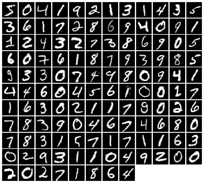
A variable NUM_TRAIN with a value of 50000 is defined, and a variable NUM_VAL with a value of 5000 is defined. The training and validation datasets are sorted by the number of samples in each column. A noise vector that has 96 dimensions is defined next with the variable NOISE_DIM. Afterward, the variable batch_size is defined with the value 128, which indicates the number of samples that will be loaded simultaneously in each batch. Next, MNIST dataset is loaded using dset.MNIST with the specified directory and transform function. When a dataset is selected for training, the data is downloaded if it has not already been saved.
The data loader with the dataset and batch size is created next, as well as a custom sampler called ChunkSampler. An array of chunks from a dataset is randomly sampled using the ChunkSampler class. The same process is repeated for the validation dataset, creating another DataLoader with the corresponding sampler that will randomly sample a chunk of data from the validation dataset. By using the functions iter and next, the first batch of training data is retrieved from the DataLoader. As a next step, the data is converted into a numpy array, reshaped to have a batch size of 128 and flattened to have dimensions of 784. Show_images displays the batch images using this data. Each batch in the dataset is processed in this manner.
Random Noise Generation
For generating random noise, create uniform noise ranging between -1 and 1. The noise should have a shape defined by [batch_size, dim].
You will need to implement the sample_noise function located in cs231n/gan_pytorch.py.
As a tip, consider using torch.rand for this task. It’s important to ensure that the generated noise is in the correct shape and type to be effectively utilized in your GAN implementation.
from cs231n.gan_pytorch import sample_noise

def test_sample_noise():
    batch_size = 3
    dim = 4
    torch.manual_seed(231)
    z = sample_noise(batch_size, dim)
    np_z = z.cpu().numpy()
    assert np_z.shape == (batch_size, dim)
    assert torch.is_tensor(z)
    assert np.all(np_z >= -1.0) and np.all(np_z <= 1.0)
    assert np.any(np_z < 0.0) and np.any(np_z > 0.0)
    print('All tests passed!')

test_sample_noise()
From the package cs231n, the function sample_noise is imported from the module gan_pytorch. Sample_noise takes in two parameters, batch_size and dim. It is determined by these parameters that the output will be a tensor containing random noise values. For reproducibility, Pytorch’s manual seed is set to 231. Afterwards, the tensor is converted to a numpy array, which is checked for shape and range within the desired range. Upon completion, a message indicating the success of all tests is printed. To ensure that the random noise generated by the sample_noise function meets the desired criteria, this code generates a batch of random noise.
Flatten and Unflatten Operations
Remember the Flatten operation we used in previous notebooks. In addition to that, this time we are including an Unflatten operation, which could be particularly useful when you are working on implementing the convolutional generator. Additionally, we have provided a weight initializer that utilizes Xavier initialization. This is a shift from PyTorch’s standard uniform initialization, and it has already been applied for your convenience.
CPU and GPU Usage
The default setting for running the code in this assignment is on a CPU. While GPUs are not essential for this assignment, they can significantly speed up the training of your models. If you prefer to utilize a GPU, you can do so by modifying the dtype variable in the upcoming cell. For those using Colab, it's advisable to switch the Colab runtime to GPU for more efficient processing.
dtype = torch.FloatTensor
#dtype = torch.cuda.FloatTensor ## UNCOMMENT THIS LINE IF YOU'RE ON A GPU!
Python code assigns variable dtype to type torch.FloatTensor. As a result, any variable with this type will be a floating point tensor. There is a comment outlining the next line, which means it will not be executed unless the comment is removed. A remove of the comment will instead replace the variable dtype with torch.cuda.FloatTensor. Using this type, GPU-calculated tensors are greatly sped up when performing calculations.
Building the Discriminator
The first task is to construct the discriminator. You’ll need to define the architecture within the nn.Sequential constructor in the provided function. Make sure all fully connected layers include bias terms. The architecture should consist of the following components:
A fully connected layer with an input size of 784 and an output size of 256.
A LeakyReLU activation function with alpha set to 0.01.
Another fully connected layer, this time with an input size of 256 and an output size of 256.
A second LeakyReLU activation, also with alpha set to 0.01.
A final fully connected layer with an input size of 256 and an output size of 1.
Remember, the Leaky ReLU activation function is defined as f(x) equals the maximum of alpha times x and x, with a constant alpha. In this case, we are using alpha equals 0.01.
The output from the discriminator should have a shape of [batch size, 1]. It will provide real number scores that indicate how likely each of the batch size inputs is to be a real image.
Test to make sure the number of parameters in the discriminator is correct:
from cs231n.gan_pytorch import discriminator

def test_discriminator(true_count=267009):
    model = discriminator()
    cur_count = count_params(model)
    if cur_count != true_count:
        print('Incorrect number of parameters in discriminator. Check your achitecture.')
    else:
        print('Correct number of parameters in discriminator.')

test_discriminator()
In this code, the discriminator function is imported from the cs231n package. Defines a new function, test_discriminator, with a parameter true_count, a value of 267009 by default. A variable model is created by calling the discriminator function within the function. As a result of this model, we will be testing the discriminator network. A number of parameters is then returned from the model by calling the count_params function.
A value of this type is stored in the cur_count variable. This is followed by an if statement that compares the variable cur_count to the optional parameter true_count. Discriminator parameters are incorrect if they are not equal, and an error message is printed. This will print a message stating that the parameters are correct if they are equal. Last but not least, the test_discriminator function is called without any arguments, which runs the function using the true_count default value and prints the appropriate message.
