

Facial Emotion Recognition with using CNN
Facial expressions serve as a crucial mode of communication among humans.

In artificial intelligence research, deep learning techniques have emerged as powerful tools for enhancing human-computer interactions. The analysis and evaluation of facial expressions and emotions in psychology involve assessing decisions to anticipate an individual’s or a group’s emotions. This study aims to develop a system capable of predicting and classifying facial emotions using the Convolutional Neural Network (CNN) algorithm and feature extraction techniques.
The process consists of three main stages: data preprocessing, facial feature extraction, and facial emotion classification. By employing the Convolutional Neural Network (CNN) algorithm, the system accurately predicted facial expressions with a 62.66% success rate. The algorithm’s performance was assessed using the FER2013 database, a publicly available dataset containing 35,887 48x48 grayscale face images, each representing a distinct emotion.
Now let’s start with the coding.
!pip install scikit-plotThis code installs the scikit-plot package using pip, which is a Python package that provides a range of useful tools for visualizing the performance of machine learning models. Specifically, scikit-plot provides a variety of functions for generating common plots used in model evaluation, such as ROC curves, precision-recall curves, confusion matrices, and more.
After executing the command “!pip install scikit-plot” in a Python environment, you should be able to import and use the scikit-plot functions in your code.
import pandas as pd
import numpy as np
import scikitplot
import random
import seaborn as sns
import keras
import os
from matplotlib import pyplot
import matplotlib.pyplot as plt
import tensorflow as tf
from tensorflow.keras.utils import to_categorical
import warnings
from tensorflow.keras.models import Sequential
from keras.callbacks import EarlyStopping
from keras import regularizers
from keras.callbacks import ModelCheckpoint,EarlyStopping
from tensorflow.keras.optimizers import Adam,RMSprop,SGD,Adamax
from keras.preprocessing.image import ImageDataGenerator,load_img
from keras.utils.vis_utils import plot_model
from keras.layers import Conv2D, MaxPool2D, Flatten,Dense,Dropout,BatchNormalization,MaxPooling2D,Activation,Input
from sklearn.model_selection import train_test_split
from sklearn.preprocessing import StandardScaler
warnings.simplefilter("ignore")
from keras.models import Model
from sklearn.model_selection import train_test_split
from sklearn.metrics import accuracy_score
from keras.regularizers import l1, l2
import plotly.express as px
from matplotlib import pyplot as plt
from sklearn.metrics import confusion_matrix
from sklearn.metrics import classification_report
The code imports various Python libraries and modules that are commonly used in machine learning and deep learning tasks. These libraries include pandas, numpy, scikit-plot, random, seaborn, keras, os, matplotlib, tensorflow, and scikit-learn.
Each import statement imports a specific set of tools or functions that are needed to perform machine learning or deep learning tasks, such as data manipulation, data visualization, model building, and performance evaluation.
Overall, this code prepares the necessary tools and modules needed to perform various machine learning and deep learning tasks, such as data preprocessing, model training, and model evaluation.
Loading The Dataset
data = pd.read_csv("../input/fer2013/fer2013.csv")
data.shape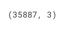
This code reads a CSV file named “fer2013.csv” located in the “../input/fer2013/” directory using pandas’ read_csv() function and assigns the resulting DataFrame to a variable called data.
The shape attribute is then called on the DataFrame to retrieve its dimensions, which returns a tuple of the form (rows, columns). This line of code will output the number of rows and columns in the DataFrame data.
data.isnull().sum()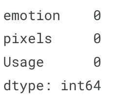
This code will return the sum of all missing values in each column of the data DataFrame.
The isnull() method of a DataFrame returns a boolean DataFrame that indicates whether each element in the original DataFrame is missing or not. The sum() method is then applied to this boolean DataFrame, which returns the sum of missing values in each column.
This is a quick way to check if there are any missing values in the DataFrame. If there are missing values, they may need to be imputed or removed before the data can be used for modeling.
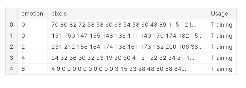
data.head()This code will return the first 5 rows of the data DataFrame.
The head() method of a DataFrame returns the first n rows (by default, n=5) of the DataFrame. This is a useful method to get a quick glimpse of the data in the DataFrame, especially when working with large datasets.
The output will show the first 5 rows of the data DataFrame, which may include the column names and the first few rows of data, depending on the structure of the DataFrame.
Data Pre-Processing
CLASS_LABELS  = ['Anger', 'Disgust', 'Fear', 'Happy', 'Neutral', 'Sadness', "Surprise"]
fig = px.bar(x = CLASS_LABELS,
             y = [list(data['emotion']).count(i) for i in np.unique(data['emotion'])] ,
             color = np.unique(data['emotion']) ,
             color_continuous_scale="Emrld")
fig.update_xaxes(title="Emotions")
fig.update_yaxes(title = "Number of Images")
fig.update_layout(showlegend = True,
    title = {
        'text': 'Train Data Distribution ',
        'y':0.95,
        'x':0.5,
        'xanchor': 'center',
        'yanchor': 'top'})
fig.show()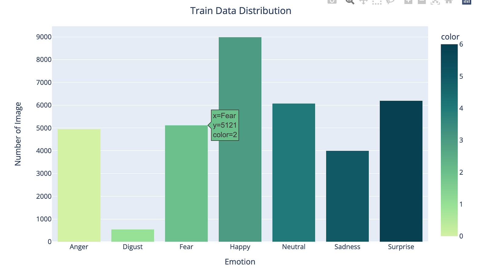
This code uses the Plotly Express library to create a bar chart that shows the distribution of emotions in the data DataFrame.
First, a list of class labels is defined in CLASS_LABELS, which corresponds to the different emotions in the dataset.
Then, the px.bar() function is called, with the x-axis representing the class labels, and the y-axis representing the number of images for each emotion. The color parameter is set to the different emotion classes, and the color_continuous_scale parameter is set to "Emrld", which is a predefined color scale in Plotly Express.
Next, various update_ methods are called to modify the layout and appearance of the plot. For example, update_xaxes() and update_yaxes() are used to set the x-axis and y-axis titles, respectively. update_layout() is used to set the plot title and its position.
Finally, the show() method is called on the figure object to display the plot.
The output will show a bar chart that displays the number of images for each emotion in the data DataFrame, with each emotion color-coded according to the color scale specified.
Shuffling Data
data = data.sample(frac=1)The sample() method of a DataFrame is used to randomly sample a fraction of the rows in the DataFrame, with frac specifying the fraction of rows to return (in this case, frac=1, which means all rows will be returned). When frac=1, the sample() method effectively shuffles the rows in the DataFrame.
This is a common operation in machine learning and deep learning tasks, where it is important to randomly shuffle the data to prevent any bias that may be introduced if the data has any inherent ordering or structure.
One Hot Encoding
labels = to_categorical(data[['emotion']], num_classes=7)to_categorical() takes two arguments: the column to be one-hot encoded and the number of classes in the data. In this case, the emotion column of the data DataFrame is passed as the first argument, and the number of classes (which is 7, corresponding to the 7 different emotions in the data) is passed as the second argument.
The output is a numpy array with a shape of (n_samples, n_classes), where n_samples is the number of samples in the DataFrame, and n_classes is the number of unique classes in the data (which is 7 in this case). Each row of the array represents a one-hot encoded label for a single sample in the data DataFrame.
train_pixels = data["pixels"].astype(str).str.split(" ").tolist()
train_pixels = np.uint8(train_pixels)
This code preprocesses the pixel values in the pixels column of the data DataFrame.
First, the astype() method is used to convert the pixels column to a string data type, which allows the split() method to be called on each row of the column.
Next, the split() method is called on each row of the pixels column to split the pixel values into a list of strings. The resulting list is then converted to a numpy array using tolist().
Finally, np.uint8() is called on the numpy array to convert the pixel values from strings to unsigned 8-bit integers, which is the datatype commonly used to represent image pixel values.
The output is a numpy array with a shape of (n_samples, n_pixels), where n_samples is the number of samples in the DataFrame, and n_pixels is the number of pixels per image in the data. Each row of the array represents the pixel values of a single image in the data DataFrame.
Standardization
pixels = train_pixels.reshape((35887*2304,1))This code reshapes the train_pixels numpy array from a 3-dimensional array of shape (n_samples, n_rows, n_columns) to a 2-dimensional array of shape (n_samples * n_rows, 1).
The reshape() method of a numpy array is used to change its shape. In this case, the train_pixels array is flattened by reshaping it into a 2D array with one column.
The resulting pixels array has a shape of (n_samples * n_rows, 1), where n_samples is the number of samples in the DataFrame, n_rows is the number of rows per image, and 1 represents the flattened pixel values of each image in the DataFrame. Each row of the array represents a single pixel value of a single image in the DataFrame.
scaler = StandardScaler()
pixels = scaler.fit_transform(pixels)
This code applies standardization to the pixels numpy array using scikit-learn's StandardScaler() function.
The StandardScaler() function is a pre-processing step that scales each feature of the data (in this case, each pixel value) to have a mean of 0 and a variance of 1. This is a commonly used technique in machine learning and deep learning tasks to ensure that each feature contributes equally to the model.
The fit_transform() method of the StandardScaler() object is then called on the pixels numpy array, which computes the mean and standard deviation of the data and scales the data accordingly. The resulting scaled data is then assigned back to the pixels numpy array.
The output is a numpy array of the same shape as the original pixels array, but with each pixel value standardized.
Reshaping the data (48,48)
pixels = train_pixels.reshape((35887, 48, 48,1))This code reshapes the train_pixels numpy array from a 2-dimensional array of shape (n_samples * n_rows, 1) to a 4-dimensional array of shape (n_samples, n_rows, n_columns, n_channels).
The reshape() method of a numpy array is used to change its shape. In this case, the train_pixels array is reshaped into a 4D array with 1 channel.
The resulting pixels array has a shape of (n_samples, n_rows, n_columns, n_channels), where n_samples is the number of samples in the DataFrame, n_rows is the number of rows per image, n_columns is the number of columns per image, and n_channels represents the number of color channels in each image.
Since the original dataset is grayscale, n_channels is set to 1. Each element of the pixels array represents the pixel value of a single grayscale image in the DataFrame.
Train test validation split
Now, we have 35887 images with each containing 48x48 pixels. We will split the data into train,test and Validation data to feed and evaluate and validate our data with the ratio of 10%.
X_train, X_test, y_train, y_test = train_test_split(pixels, labels, test_size=0.1, shuffle=False)
X_train, X_val, y_train, y_val = train_test_split(X_train, y_train, test_size=0.1, shuffle=False)
This code splits the preprocessed image data pixels and one-hot encoded labels labels into training, validation, and test sets using scikit-learn's train_test_split() function.
The train_test_split() function randomly splits the data into training and testing subsets based on the test_size parameter, which specifies the fraction of the data that should be used for testing. In this case, test_size=0.1, which means that 10% of the data will be used for testing.
The shuffle parameter is set to False to preserve the original order of the samples in the DataFrame.
The resulting X_train, X_val, and X_test arrays contain the pixel values of the training, validation, and test sets, respectively. The y_train, y_val, and y_test arrays contain the one-hot encoded labels for the corresponding sets.
The training set is further split into training and validation sets using train_test_split() again, with test_size=0.1. This splits the data into 80% for training, 10% for validation, and 10% for testing.
print(X_train.shape)
print(X_test.shape)
print(X_val.shape)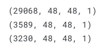
These lines of code print the shapes of the X_train, X_test, and X_val arrays after splitting the data into training, validation, and test sets.
The shape attribute of a numpy array returns a tuple of the array's dimensions. In this case, the shapes of the X_train, X_test, and X_val arrays will depend on the number of samples in each set and the dimensions of each sample.
The output will display the shapes of the arrays in the format (n_samples, n_rows, n_columns, n_channels), where n_samples is the number of samples in the set, n_rows is the number of rows per image, n_columns is the number of columns per image, and n_channels represents the number of color channels in each image.
We can see some train data containing one sample of each class with the help of this plot code.
plt.figure(figsize=(15,23))
label_dict = {0 : 'Angry', 1 : 'Disgust', 2 : 'Fear', 3 : 'Happiness', 4 : 'Sad', 5 : 'Surprise', 6 : 'Neutral'}
i = 1
for i in range (7):
    img = np.squeeze(X_train[i])
    plt.subplot(1,7,i+1)
    plt.imshow(img)
    index = np.argmax(y_train[i])
    plt.title(label_dict[index])
    plt.axis('off')
    i += 1
plt.show()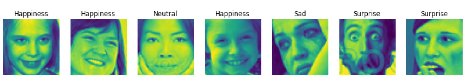
This code creates a 7x1 subplot grid of images from the training set using matplotlib’s plt.subplots() function.
The squeeze() method of numpy arrays is used to remove any single-dimensional entries from the shape of the arrays, effectively converting a 4D array into a 3D array.
For each subplot, the imshow() function is used to display the corresponding image, and the title() function is used to display the corresponding label.
The axis() function is used to turn off the axis for each subplot.
The output is a visualization of the first 7 images in the training set, along with their corresponding labels.
Data augmentation using ImageDataGenerator
We can do data augmentation to have more data to train and validate our model to prevent overfitting. Data augmentation can be done on training and validation sets as it helps the model become more generalize and robust.
datagen = ImageDataGenerator(  width_shift_range = 0.1,
                               height_shift_range = 0.1,
                               horizontal_flip = True,
                               zoom_range = 0.2)
valgen = ImageDataGenerator(   width_shift_range = 0.1,
                               height_shift_range = 0.1,
                               horizontal_flip = True,
                               zoom_range = 0.2)
This code creates two ImageDataGenerator objects, datagen and valgen, which will be used for data augmentation during training and validation.
The ImageDataGenerator class is a Keras pre-processing utility that performs various types of image augmentation in real-time, such as shifting, flipping, rotating, and zooming.
The datagen object includes a number of augmentation techniques:
width_shift_rangeandheight_shift_rangerandomly shift the image horizontally and vertically by a maximum of 10% of the image width and height, respectively.horizontal_fliprandomly flips the image horizontally.zoom_rangerandomly zooms the image by a factor of up to 20%.
The valgen object includes the same augmentation techniques as datagen, but will be applied only to the validation set during training.
By applying data augmentation during training, the model will be exposed to a larger and more diverse set of training data, which can help prevent overfitting and improve the model’s ability to generalize to new data.
datagen.fit(X_train)
valgen.fit(X_val)
These lines of code fit the ImageDataGenerator objects datagen and valgen to the training and validation data, respectively.
The fit() method of an ImageDataGenerator object computes any internal statistics required to perform the data augmentation, such as mean and variance of pixel values. In this case, the fit() method is called on datagen and valgen with the training and validation sets as input to compute these statistics.
After the ImageDataGenerator objects are fitted to the data, they can be used to apply data augmentation in real-time during training and validation.
train_generator = datagen.flow(X_train, y_train, batch_size=64)
val_generator = datagen.flow(X_val, y_val, batch_size=64)
These lines of code create two ImageDataGenerator iterators, train_generator and val_generator, which can be used to generate batches of augmented data during training and validation.
The flow() method of an ImageDataGenerator object takes in numpy arrays of input data and labels, and generates batches of augmented data on-the-fly.
In this case, train_generator is created using the flow() method on datagen, with the training data X_train and y_train as input, and a batch size of 64. val_generator is created using the same method on valgen, with the validation data X_val and y_val as input, and a batch size of 64.
During training, the train_generator the iterator will be used to generate batches of augmented data on-the-fly for each training epoch. Similarly, the val_generator the iterator will be used to generate batches of augmented data for each validation epoch.
Code Download
Download the code using the link below. Only paid subscribers can download the entire code. And also access the rest of the article. So please consider becoming a paid subscriber, and get access to everything I publish on my newsletter and on youtube. Every Source code and Every Dataset.
