Forecasting Stock Performance with Prophet
The stock market has always captivated investors, economists, and financial analysts.

Predicting stock performance remains a challenge, but recent advancements in machine learning and data science offer sophisticated forecasting techniques to aid decision-making.
In this article, we’ll explore how Facebook’s open-source library, Prophet, can forecast stock performance using time series data, focusing on the historical daily S&P 500 adjusted close prices. We’ll provide a detailed walkthrough on creating a three-year forecast using year-to-date data and simulate historical monthly forecasts dating back to 1980, examining our model’s accuracy and reliability.
Additionally, we’ll discuss various trading strategies that utilize Prophet-powered predictions and compare them to the classic buy-and-hold approach, highlighting the most effective methods for maximizing returns in the volatile stock market.
In this post we will be using Prophet to forecast time series data. The data we will be using is historical daily SA&P 500 adjusted close price. We will first create a 3 year forecast usind ytd data and then simulate historical monthly forecasts dating back to 1980. Finally we will create various trading strategies to attempt to beat the tried and true method of buying and holding.
Sections:
* Imports
* Data Preparation
* Prophet
* Simulating Forecasts
* Trading Algorithms
* Summary
Imports
import pandas as pd
import numpy as np
from fbprophet import Prophet
import matplotlib.pyplot as plt
from functools import reduce

%matplotlib inline
import warnings
warnings.filterwarnings('ignore')

plt.style.use('seaborn-deep')
pd.options.display.float_format = "{:,.2f}".format
To forecast and manipulate time series data, this code imports necessary libraries.
Using pandas as a library, the first line of code imports it. Python’s Pandas library is a popular data analysis and manipulation tool. Numpy library is imported as np in the second line. The NumPy library is a powerful tool for scientific computation and working with arrays.
Thirdly, Prophet is imported from the Facebook Prophet package. The Prophet library is an open-source library developed by Facebook to forecast time series.
Matplotlib’s pyplot module and functools’ reduce method are imported for displaying data and applying functions cumulatively.
To display matplotlib plots in output cells of Jupyter Notebook, the next line uses the %matplotlib inline command.
Plots are styled and float values are formatted in the last three lines of code. To give the plots a dark background and deep colors, the seaborn-deep style is set using plt.style.use(). A float value in a pandas dataframe will have two decimal places if pd.options.display.float_format is set to two. Last but not least, warnings.filterwarnings(‘ignore’) suppresses any warnings generated during program execution.
The Data
stock_price = pd.read_csv('^GSPC.csv',parse_dates=['Date'])In this code, we read data from a CSV file named GSPC.csv into a pandas dataframe called stock_price using the pandas library. pd.read_csv() returns a dataframe from a CSV file.
Pandas interprets the ‘Date’ column as a date and time data type when parse_dates is set to [‘Date’]. Time series analysis benefits from this because it makes it easier to work with the time component.
With each row representing a day in the stock market, the resulting dataframe contains the data from the CSV file. Date, Open, High, Low, Close, Adjust Close, and Volume are the columns of the dataframe. For each day, these columns contain information about the opening price, high price, low price, closing price, adjusted closing price, and volume of trading.
stock_price.info()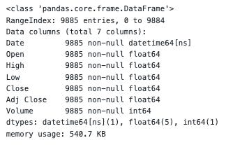
Stock_price.info() displays a summary of each column in the DataFrame stock_price, including its data types, non-null values, and memory usage.
The output is:
Stock_price is a pandas DataFrame object with 9885 rows and 7 columns, as shown by stock_price.info().
Each column in the DataFrame is summarized in the Data columns section of the output:
Stock prices are recorded using a column of datetime values.
On each corresponding date, these columns contain float values representing the stock market’s opening, highest, lowest, closing, and adjusted closing prices.
The volume of the stock market on each date is represented by a column of integer values.
Each column in the DataFrame is listed by its data type in the dtypes section. Date columns have the datetime64[ns] data type, which indicates they contain datetime values. A float64 data type indicates that the Open, High, Low, Close, and Adj Close columns contain floating-point values. There are integer values in the Volume column because it has the int64 data type.
In the memory usage section, you can see how much memory the DataFrame uses in kilobytes (KB). Currently, 540.7 KB of memory is being used by the DataFrame.
As a result, this output provides useful information about the structure and content of the stock_price DataFrame. It confirms that all columns have the expected data types and that there are no missing values in the DataFrame.
Data Preparation
stock_price = stock_price[['Date','Adj Close']]A subset of columns is selected from the stock_price dataframe using this code. In particular, it selects the columns ‘Date’ and ‘Adj Close’, which contain the date and adjusted closing price of the stock market each day.
There are only two columns in the resulting dataframe, “Date” and “Adj Close,” and the number of rows remains the same as in the original dataframe. As we can focus on the trend of the adjusted closing price over time, this subset of data is useful for time series analysis and forecasting.
stock_price.columns = ['ds', 'y']
stock_price.head(10)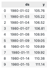
The stock_price DataFrame is renamed and the first 10 rows of the updated DataFrame are displayed.
Each part of the code does the following:
Stock_price.columns = [‘ds’, ‘y’]: Renames the stock_price DataFrame column labels to ds and y. Column names are assigned to the DataFrame’s columns attribute using its columns attribute.
This function displays the first 10 rows of the updated stock_price DataFrame.
This code updates the column labels of the stock_price DataFrame to match the Prophet time-series forecasting model’s expected input format. Specifically, ds is the column that should contain the time series dates as a pandas datetime object, and y is the column that should contain the forecasted values. To verify that the column labels have been updated correctly, and to inspect the first few rows of the updated DataFrame, we use the head() method.
For prophet to work, we need to change the names of the ‘Date’ and ‘Adj Close’ columns to ‘ds’ and ‘y’. The term ‘y’ is typically used for the target column (what you are trying to predict) in most machine learning projects.
Prophet
stock_price.set_index('ds').y.plot(figsize=(12,6), grid=True);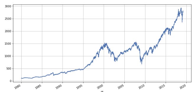
In this code, stock_price.set_index(‘ds’).y.plot(figsize=(12,6), grid=True); plots the historical value of the S&P 500 index as a line plot.
A DataFrame is first set up with the index set as ‘ds’ by calling the set_index() method with the ds argument. DataFrames are created by using dates as their indexes.
A line plot of the time series is generated by calling the plot() method on the y column of the updated DataFrame. This plot is 12 inches wide by 6 inches tall because the figsize parameter is set to (12,6). Grid parameter is set to True, which adds a grid to the plot for easier visualization.
Finally, the semicolon ; suppresses any text output generated by the plot() method, allowing the plot to stand alone.
As a result, this line plot can help identify trends and patterns in the S&P 500 index over time, such as seasonality, cyclical fluctuations, or long-term growth or decline. It is easy to see how the value of the index changes over time when the x-axis shows the date and the y-axis shows the value of the index.
Before we use Prophet to create a forecast let’s visualize our data. It’s always a good idea to create a few visualitions to gain a better understanding of the data you are working with.
model = Prophet()
model.fit(stock_price)
In this code, a new instance of the Prophet class is created and the time series data from the stock_price DataFrame is fitted to the model.
Each part of the code does the following:
Creates an instance of the Prophet class, which is a Facebook-developed time-series forecasting model. Prophet uses a generalized additive model approach to capture both linear and non-linear trends in the data, as well as seasonality and holiday effects.
The stock_price DataFrame is fitted to the Prophet model using the fit() method by model.fit(stock_price). Using historical data, the model is trained to predict future data.
A new Prophet model is created and fitted to the stock_price DataFrame, which enables the model to learn from historical data and forecast future prices.
To activate the Prophet Model we simply call `Prophet()` and assign it to a variabl called `model`. Next fit our stock data to the model by calling the `fit` method.
future = model.make_future_dataframe(1095, freq='d')

future_boolean = future['ds'].map(lambda x : True if x.weekday() in range(0, 5) else False)
future = future[future_boolean]

future.tail()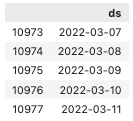
The code future = model.make_future_dataframe(1095, freq=’d’); future_boolean = future[‘ds’].map(lambda x : True if x.weekday() in range(0, 5) otherwise False); future = future[future_boolean]; future.tail() creates a new pandas DataFrame called future that contains a range of future dates for which the Prophet model will make predictions.
First, the make_future_dataframe() method is invoked on the Prophet model object with the arguments 1095, which specifies the number of days to forecast, and freq=’d’, which specifies the frequency of the dates.
Following that, the dates in future are filtered to include only weekdays using a Boolean array called future_boolean. On the ds column of the future DataFrame, the map() method is called to create a new array containing True for weekdays (days with a weekday index between 0 and 4 inclusive) and False for weekends (days with a weekday index between 5 and 6 inclusive).
By removing all weekends from the DataFrame, the filtered future DataFrame includes only rows where future_boolean is True.
A final call to tail() on the filtered future DataFrame displays the last few rows, which contain the predictions made by the Prophet model for the future weekdays.
A new DataFrame called future is created, containing a range of future dates for which the Prophet model will predict. Using the code, the model will only make predictions for days when the stock market is open by filtering the dates to include only weekdays.
To create a forecast with our model we need to create some futue dates. Prophet provides us with a helper function called `make_future_dataframe`. We pass in the number of future periods and frequency. Above we created a forecast for the next 1095 days or 3 years.
Since stocks can only be traded on weekdays we need to remove the weekends from our forecast dataframe. To do so we create a boolean expression where if a day does not equal 0–4 then return False. “0 = Monday, 6=Saturday, etc..”
We then pass the boolean expression to our dataframe with returns only True values. We now have a forecast dataframe comprised of the next 3 years of weekdays.
model.plot(forecast);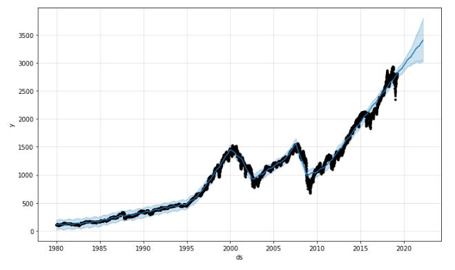
It shows a plot of the forecast DataFrame, together with the historical data from the stock_price DataFrame used to fit the Prophet model, as well as predicted values for the S&P 500 index over time.
Using this code, you can:
This method generates a plot of the forecast DataFrame, showing the predicted values for the S&P 500 index over time along with the historical data from the stock_price DataFrame that was used to fit the Prophet model. A DataFrame with predicted values is specified with the argument forecast to the plot() method on the Prophet model object.
As a result, a black line shows historical stock price data, and a blue line shows predicted S&P 500 values. Around the blue line, the shaded blue area represents the uncertainty intervals for the predicted values, with the light blue area representing the 80% confidence interval and the dark blue area representing the 95% confidence interval. During the fitting process, the Prophet model also identified trend, seasonality, and holiday components.
We can visualize the trends and patterns in the predicted values by comparing them to the historical values using this code, which generates a plot of the predicted values for the S&P 500 index over time.
model.plot_components(forecast);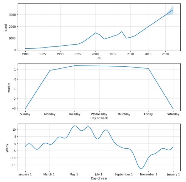
Based on the predicted values contained in the forecast DataFrame, this code generates plots showing trend, seasonality, and holiday components of the Prophet model.
Using this code, you can:
Based on prediction values contained in the forecast DataFrame, model.plot_components(forecast) generates a set of plots showing trend, seasonality, and holiday components. Prophet model objects are passed forecast as the argument to plot_components(), which returns a DataFrame containing predicted values.
A black line represents the trend component of the model, while a blue line represents the seasonality component. A plot of the yearly and weekly seasonality components is shown in the first plot. Monthly seasonality is shown in the second plot, while daily seasonality is shown in the third plot. With each holiday represented as a separate line in the fourth plot, we can see how holidays affect predicted values.
Based on the predicted values contained in the forecast DataFrame, this code generates a set of plots that visualize the trend, seasonality, and holiday components of the Prophet model. We can use this information to better understand the factors that drive the predicted values of the S&P 500 index over time.
All the new fields appear a bit daunting but fortunately Prophet comes with two handy visualization helpers, `plot` and `plot_components`. The `plot` functions creates a graph of our actuals and forecast and `plot_components` provides us a graph of our trend and seasonality.
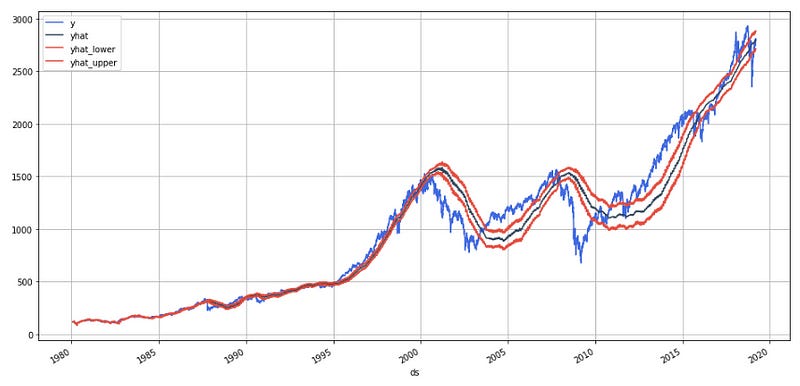
stock_price_forecast = forecast[['ds', 'yhat', 'yhat_lower', 'yhat_upper']]
df = pd.merge(stock_price, stock_price_forecast, on='ds', how='right')
df.set_index('ds').plot(figsize=(16,8), color=['royalblue', "#34495e", "#e74c3c", "#e74c3c"], grid=True);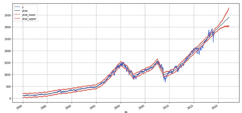
This code creates a new DataFrame called df that combines the historical data from the stock_price DataFrame with the predicted values from the forecast DataFrame, and then generates a line plot of the historical and predicted values over time.
Here’s what this code does:
stock_price_forecast = forecast[[‘ds’, ‘yhat’, ‘yhat_lower’, ‘yhat_upper’]]: Creates a new DataFrame called stock_price_forecast that contains the predicted values for the S&P 500 index, extracted from the forecast DataFrame. This DataFrame contains columns for the ds (date) column, as well as the yhat (forecasted value), yhat_lower (lower bound of the predicted interval), and yhat_upper (upper bound of the predicted interval) columns.
df = pd.merge(stock_price, stock_price_forecast, on=’ds’, how=’right’): Merges the historical data from the stock_price DataFrame with the predicted values from the stock_price_forecast DataFrame, using the ds (date) column as the key. The resulting df DataFrame contains columns for the ds (date), y (actual historical value), yhat (forecasted value), yhat_lower (lower bound of the predicted interval), and yhat_upper (upper bound of the predicted interval).
df.set_index(‘ds’).plot(figsize=(16,8), color=[‘royalblue’, “#34495e”, “#e74c3c”, “#e74c3c”], grid=True): Generates a line plot of the historical and predicted values over time, using the df DataFrame. The set_index() method is called on the df DataFrame to set the ds (date) column as the index. The plot() method is then called on the resulting DataFrame, with the argument figsize=(16,8) specifying the size of the plot, and the argument color=[‘royalblue’, “#34495e”, “#e74c3c”, “#e74c3c”] specifying the colors of the lines for the historical data, forecasted values, and uncertainty intervals. The argument grid=True adds a grid to the plot for easier visualization.
The resulting plot shows the historical data from the stock_price DataFrame as a blue line, with the predicted values for the S&P 500 index shown as a red line. The shaded red area around the red line represents the uncertainty intervals for the predicted values, with the lighter red area representing the 80% confidence interval and the darker red area representing the 95% confidence interval. The plot allows us to visualize how well the Prophet model fits the historical data, as well as how well it predicts the future values of the S&P 500 index.
Simulating Forecast
Our 3-year forecast is pretty cool, but we want to backtest it and develop a trading strategy before making any trading decisions.
This section simulates Prophet’s existence back in 1980 and uses it to create a monthly forecast through 2019. The following section will simulate how various trading strategies performed compared to buying and holding a stock.
stock_price['dayname'] = stock_price['ds'].dt.day_name()
stock_price['month'] = stock_price['ds'].dt.month
stock_price['year'] = stock_price['ds'].dt.year
stock_price['month/year'] = stock_price['month'].map(str) + '/' + stock_price['year'].map(str)

stock_price = pd.merge(stock_price,
                       stock_price['month/year'].drop_duplicates().reset_index(drop=True).reset_index(),
                       on='month/year',
                       how='left')

stock_price = stock_price.rename(columns={'index':'month/year_index'})
As part of this code, we add four new columns to the stock_price DataFrame that contain information about the date in the ds column.
In the stock_price DataFrame, the first line creates a column called dayname that contains the day of the week (e.g., Monday, Tuesday) corresponding to each date in the ds column. Datetime properties are accessed using the .dt attribute, and the day_name() method returns the day name.
A new column, month, is created in the stock_price DataFrame to store the month of each date in the ds column (as a number between 1 and 12). Datetime objects can be accessed by their month value using the dt attribute.
In the stock_price DataFrame, the third line creates a new column called year that contains the year corresponding to each date. This time, the datetime object’s year value can be accessed using the dt attribute.
With the fourth line, the month and year columns are concatenated as strings in the stock_price DataFrame, separated by a forward slash (/). DataFrames created this way have unique identifiers for each month/year combination.
A single row is created for each unique month/year combination in the stock_price DataFrame with the help of the pd.merge() function in the fifth line. Each unique month/year combination is indexed by its unique integer index in the resulting DataFrame, which has an additional column called index.
As a final step, the dataframe’s index column is renamed to month/year_index in order to be more clear about the fact that this column contains unique integer indexes for each unique combination of month and year.
stock_price.tail()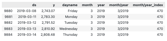
As a result of the stock_price.tail() method, the last five rows of the stock_price DataFrame are displayed. In this way, the previous transformations can be checked and verified quickly.
As a result of the tail() function, we receive the last five rows of the stock_price DataFrame, containing the columns ds (date), y (adjusted closing price), dayname, month, year, month/year, and month/year_index.
Tail() can be used to check whether the new columns were correctly added to the DataFrame and whether the data is sorted in the right order by date. Furthermore, the output can provide insight into the overall structure and patterns of the data, such as gaps or outliers.
Generally, the tail() function is useful for verifying that any previous transformations have been applied correctly.
Before we simulate the monthly forecasts we need to add some columns to our `stock_price` dataframe we created in the beginning of this project to make it a bit easier to work with. We add month, year, month/year, and month/year_index.
loop_list = stock_price['month/year'].unique().tolist()
max_num = len(loop_list) - 1
forecast_frames = []

for num, item in enumerate(loop_list):

    if  num == max_num:
        pass
    else:
        df = stock_price.set_index('ds')[
             stock_price[stock_price['month/year'] == loop_list[0]]['ds'].min():\
             stock_price[stock_price['month/year'] == item]['ds'].max()]

        df = df.reset_index()[['ds', 'y']]

        model = Prophet()
        model.fit(df)

        future = stock_price[stock_price['month/year_index'] == (num + 1)][['ds']]

        forecast = model.predict(future)
        forecast_frames.append(forecast)
Using Python, this code forecasts stock prices over time using a time series model. By using the tolist() method, the first line of code creates a unique list of month/year values from a column in the stock_price dataset.
Using the loop_list list as a source, the following line creates a variable named max_num. A for loop will be used later on to use this information. Using the third line, the stock price predictions are stored in an empty list called forecast_frames.
Iterating through the items in loop_list is then performed using a for loop. As a result of the enumerate() method, a tuple contains both the item’s index and its value. As well as keeping track of the current index number (num), this code also keeps track of the current item (item).
Inside the for loop, an if statement checks whether the current index is equal to max_num. The loop will move on to the next item if the pass statement is executed. The code inside the else block is executed if the current index is less than max_num.
As a first step, the else block creates a new dataset called df, which is a subset of the stock_price dataset. For each item in loop_list, the earliest and latest dates are determined by using the min() and max() methods by setting the ‘ds’ column as the index. Next, only the columns ‘ds’ and ‘y’ are included in the resulting dataframe, which is reset to the default index.
After that, a new Prophet model is created and fitted to the df dataframe using the fit() method. In Prophet, a curve is fitted to the data and predictions are made using a Bayesian approach.
In the next step, a new dataframe called future is created containing only the dates for the next item in loop_list. After making a prediction for each date in the future dataframe, it uses the predict() method of the Prophet model. Forecast_frames is then updated with the resulting forecast.
In general, this code fits a curve to a stock price dataset and makes predictions for future time periods by using the Prophet library. Using a list of unique month/year values, it creates a subset of the dataset for each month/year, fits a model to that subset, and uses the model to make predictions for the next time period. For further analysis, forecasts are stored in a list.
df = pd.merge(stock_price[['ds','y', 'month/year_index']], stock_price_forecast, on='ds')
df['Percent Change'] = df['y'].pct_change()
df.set_index('ds')[['y', 'yhat', 'yhat_lower', 'yhat_upper']].plot(figsize=(16,8), color=['royalblue', "#34495e", "#e74c3c", "#e74c3c"], grid=True)